
Abstract
In the paper a method for the design of the control system is presented. With the use of an evolutionary methods an initial structure of the controller is adjusted such that the designed controller fulfills the control objective in the best way possible. This elastic structure consists of basic functional blocks and filters. The proposed method is able to find such the structure and parameters of the controller, which make it immune to measurement noise that could disrupt the work of the control system. As a result, the process of controller design is performed easier and faster.
Access provided by Autonomous University of Puebla. Download conference paper PDF
Keywords
- Evolutionary optimization
- Elastic controller structure
- PID algorithm
- Structure selection
- Filter selection
1 Introduction
The problem of designing control systems is well known in science [1]. This is due to the fact that the quality of work of individual parts or even of entire machines mainly depends on the characteristics of the used controller. It should be noted that in this context, the design of the control system is not only the selection of parameters for a known controller structure. On the contrary, it is a much broader concept. Namely, the design of the control system consists of the following elements:
-
indication of measurable signals, which can be used in a feedback loop,
-
selection of the controller structure,
-
tuning of controller parameters,
-
implementation in target hardware platform with fulfillment of requirements of real-time work.
Usually these steps are performed in the presented order. If this approach does not lead to achieve the desired effect (that is, to obtain a satisfactory quality of work), then the whole procedure must be repeated starting from the second step. The controller structure needs to be modified (or completely changed) and the tuning procedure must be carried out starting from the beginning.
In the literature there are known controller structures which are typically used, they are: controllers structures based on the combination of linear correction terms, e.g. PID controllers (optionally with gain scheduling algorithm, with feed-forward path or with additional low-pass filters [2], state feedback controllers, nonlinear controllers based on computational intelligence and hybrid controllers, in which are combined approaches from other groups. However, in practice PID controllers are used the most often [1]. It is a result of widespread knowledge of how they work and their relatively simple implementation in a microprocessor-based control systems.
It is important to point out that the control system design process is difficult and time consuming. Sometimes, in order to obtain a better quality of control, an engineer, basing on his experience, has to modify the controller structure. Modification of the controller structure, usually performed by means of trial and error method, causes the process of controller design much more difficult.
Among the experimental methods for the design of control systems, methods based on artificial intelligence [17, 20–22, 25–28, 31, 38–43, 56, 63, 64] and in particular the methods of evolution [32–34] are becoming more common. The effectiveness of these methods is proven by their diversity. They include, among others, fuzzy systems [8–14, 36, 53, 54], optimization methods [5–7, 19, 22–24, 29, 30, 37, 44–52], decision trees [3, 4] and can be used in wide area of problems [15, 16, 18, 57–62, 65, 67–74]. These methods make the design of the control system easier. However, in many cases the obtained controller is sensitive to interference, which commonly occurs in the real-world conditions. The measurement noise and limited resolution of the digital word used to carry information about the measured values can lead to unstable controller operation.
In this paper it is proposed the use of low-pass finite-impulse-response filters (FIR) with programmable characteristics for each of the measurement signals used in the feedback loop. These filters are designed to suppress interference that could disrupt the work of the control system. So, it is possible to find the structure and parameters of the controller, which makes it immune to this type of interference. We suggest the use of an universal initial structure which in the process of evolution will be adjusted in a way that the designed controller fulfills the control objective in the best way possible. This elastic structure consists of basic functional blocks and filters, both with programmable connections and parameters. Due to this approach the design of the control system can be regarded as one continuous process, unlike the commonly used method of trial and error. As a result, the process of controller design is performed easier and faster. Details of the proposed method are described in Sect. 3.
This paper is organized into 5 sections. Section 2 contains a description of the extended PID controller structure, while Sect. 3 shows the proposed evolutionary algorithm used to design control system. Simulation results are presented in Sect. 4. Conclusions are drawn in Sect. 5.
2 Description of Proposed PID Controller
Proposed controller is based on elastic structure, which among the others, depends from number of controller input signals \(fb_i\), \(i=1,...,FB\), FB stands for number of feedback signals (see Fig. 1). In proposed structure assumptions that \(fb_1\) stands for desired value of \(fb_2\) and the rest of the feedback signals stand for additional measurable signals were made. Moreover, the control blocks (CB) and finite impulse response filters (FIR) can be dynamically switched off or on by changing controller parameters. Due to that, the design of the controller should not only consider selecting the real parameters of the controller but also integer parameters encoding its structure.
Proposed controller (see Fig. 1) uses typical P, I and D elements (see. respectively Fig. 2(a), (b) and (c)). These elements can be part of typical control block CB (see Fig. 2(d)). The output value of typical control block takes the following form:
where \({K^\mathrm{{P}}}\), \({K^\mathrm{{I}}}\) and \({K^\mathrm{{D}}}\) stand respectively for parameters of P, I and D elements of control block. The proposed CB structure allows for additional reduction of P, I, D elements by using integer values \(C^\mathrm{{P}}\), \(C^\mathrm{{I}}\), \(C^\mathrm{{D}}\) and reduction of whole control block by integer value \(C^\mathrm{{CB}}\). The reduction takes place if the integer values are set to 0. The output of the proposed CB takes the following form:

Proposed controller structure: (a) with any number of FB feedback signals, (b) with 3 feedback signals.

Typical structure of: (a) element P, (b) element I, (c) element D, (d) control block CB, (e) filter FIR, \(z^{-1}\) stands for values from previous time step.
The proposed FIR filters used in controller are based on typical FIR filters (see Fig. 2(e)) with using an additional integer parameter \(C^\mathrm{{F}}\) to reduction of the filter (in case of reduction the output of the filter is exact to input of the filter). Thus, the output of the proposed filter takes the following form:
where e(t) stands for input value, \(e(t-i)\) stands for input value from \(t-i\) time step, \(b_s\) stands for weights of filter, \(s=1,...,S\), S stands for length of the filter (S has to be an odd number). The weights of the filter are calculated using filter parameters: transition frequency ft and lenght of the filter S, which are a part of the elastic structure of the controller and should be selected by learning algorithm as well. The weights values \(b_s\) are calculated as follows:
The proposed controller structure is characterized by the following advantages: (a) it is able to process any number of feedback signals \(fb_i\), (b) it uses cascade control blocks configuration which allows us to obtain good accuracy of the controller, (c) the structure is dynamic, each CB block, CB block elements (P,I,D) and filter FR can be switched off or on, (d) it has great capabilities of learning due to many selectable parameters (e) it is able to minimize the impact of feedback signals noises by use of the FIR filters.
3 Description of the Proposed Algorithm
A new hybrid evolutionary algorithm is presented to select the proposed controller parameters and parameters encoding controller structure. It is based on an ensemble of genetic algorithm (to select controller structure) and evolutionary strategy (to select controller parameters). This ensemble was proposed in our previous work [33, 67] and it achieved good results. In this paper we propose a number of improvements (introduced by our experience) that may allow us to obtain even better results. These improvements are based on iteration-dependent parameters of learning algorithm, using multiple learning parameters and operators, and new encoding of the controller parameters.
3.1 Encoding of the Controller Parameters
The parameters and the structure of the proposed controller are encoded in chromosome \({\mathbf{{X}}_{ch}}\) defined as follows:
where part \({\mathbf{{X}}_{ch}^{\mathrm{{par}}}}\) encodes the real parameters of the controller and part \({\mathbf{{X}}_{ch}^{\mathrm{{str}}}}\) encodes integer parameters of the controller. The part \({\mathbf{{X}}_{ch}^{\mathrm{{par}}}}\) is defined as follows:
where \(K^\mathrm{{P}}_m\in [0, 20],K^\mathrm{{I}}_m\in [0,50],K^\mathrm{{D}}_m\in [0,5]\) stand for CB P, I, D parameters, \(m=1,...,M\), M stands for number of CB blocks, \(ft_r\in [0.1,0.5]\) stands for transition frequency, \(r=1,...,R\), R stands for number of filters, \(L^{\mathrm{{par}}}=3M+R\) stands for number of genes in part \({\mathbf{{X}}_{ch}^{\mathrm{{par}}}}\). The part \({\mathbf{{X}}_{ch}^{\mathrm{{str}}}}\) is defined as follows:
where \(C^\mathrm{{P}}_m\in \{0,1\},C^\mathrm{{I}}_m\in \{0,1\},C^\mathrm{{D}}_m\in \{0,1\}\) stand for activation of CB PID elements (values equal to 1 stands for active element), \(C^\mathrm{{CB}}_m\in \{0,1\}\) stands for activation of m-th control block, \(C^\mathrm{{F}}_r\in \{0,1\}\) stands for activation of r-th filter (values equal to 1 stands for active element), \(F_r\in \{0,...,9\}\) stands for lenght of the filter (real lenght of the filter is calculated as \(S_r = 5+2F_r\)), \(L^{\mathrm{{str}}}=4M+2R\) stands for number of genes in part \({\mathbf{{X}}_{ch}^{\mathrm{{str}}}}\).
3.2 Proposed Algorithm Description
Proposed algorithm is based on new iteration-dependent mutation and crossover from genetic algorithm and evolutionary strategy. The algorithm works according to the following steps:
-
Step 1. Initialization. In this step the value iteration is set to 0. Next the N individuals (each individual \({\mathbf{{X}}_{ch}}\) represents controller encoded by chromosome (5)) are randomly initialized and stored in population \(\mathbf {P}\). The initialization of individuals’ genes is realized as follows:
 (8)
(8)where \(U^\mathrm{{g}}(a,b)\) returns a random real value from the range [a, b].
 and
and  stand respectively for minims and maxims values of genes \(X_{ch,g}^{\mathrm{{par}}}\), \(g=1,...,L^\mathrm{{par}}\), \(U^\mathrm{{h}}(a,b)\) returns random integer value from the range [a, b].
  and
and  stand respectively for minims and maxims values of genes \(X_{ch,h}^{\mathrm{{str}}}\), \(h=1,...,L^\mathrm{{str}}\).
 -
Step 2. Evaluation. In this step each individual is evaluated by fitness function defined as follows:
$$\begin{aligned} \mathrm{{ff}}\left( {{\mathbf{{X}}_{ch}}} \right) = \sum \limits _{f = 1}^F{{\mathrm{{w}}_f} \cdot \mathrm{{ffco}}{\mathrm{{m}}_f}\left( {{\mathbf{{X}}_{ch}}} \right) }, \end{aligned}$$(9)where \({\mathrm{{ffco}}{\mathrm{{m}}_f}\left( {{\mathbf{{X}}_{ch}}} \right) }\) stands for fitness function components which depend from simulation problem (see Sect. 4.1), \(w_f\) stands for weights of fitness function components, \(f=1,...,F\), F stands for number of fitness function components.
-
Step 3. Probabilities calculation. In this step the value iteration is incremented. Next, the dynamic parameters for mutation and crossover are calculated as follows:
$$\begin{aligned} \left\{ {\begin{array}{*{20}{l}} {{p_1} = 0.2 + 0.2 \cdot \alpha }\\ {{p_2} = 0.2 \cdot \alpha }\\ {{p_3} = 0.5 \cdot \alpha }\\ {{p_4} = 0.1 \cdot \alpha }\\ {{p_5} = 0.2 \cdot \alpha \cdot \alpha } \end{array}} \right. , \end{aligned}$$(10)where \(p_1\) stands for gene mutation probability, \(p_2\) stands for gene mutation range, \(p_3\) stands for chance of select gene directly from one of parents while crossover, \(p_4\) stands for integer gene mutation probability (this value is small due to higher impact on the system), \(p_5\) stands for chance of assign random integer value into integer gene (all parameters p were estimated experimentally on the basis of experience of authors), \(\alpha \) stands for iteration-dependent value calculated as:
$$\begin{aligned} \alpha = 1 - \frac{{iteration}}{{iteratio{n^{\max }}}}. \end{aligned}$$(11)where \(iteration^{\max }\) stands for maximum number of iteration of the algorithm.
-
Step 4. Reproduction. In this step a N new individuals are created and stored in population \(\mathbf {P'}\). For each individual the condition \(U^\mathrm{{g}}(0,1)<p_c\) is checked (where \(p_c\) stands for crossover probability). If this condition is met, new individual is created as a result of crossover between two individuals selected by the roulette wheel method [55] from population \(\mathbf {P}\). Otherwise, the individual is created as a result of cloning and mutating of one individual selected by the roulette wheel method [55] from population \(\mathbf {P}\). The mutation is performed according to Eq. (13) described in detail in Step 5. The genes obtained from crossover are calculated as:
 (12)
(12)where \({X_{ch,*1}^{\mathrm{{A,*2}}}}\) and \({X_{ch,*}^{\mathrm{{B,*}}}}\) stand respectively for genes from the first and second parent, \(*1\) stands for ‘par’ or ‘str’, \(*2\) stands for ‘g’ or ‘h’. The purpose of Eq. (12) is to increase chance to select gene values directly from parents or in the other case to select gene values between gene values of parents (if condition \({{U^\mathrm{{g}}}\left( {0,1} \right) \ge {p_3}}\) is met).
-
Step 5. Mutation. In this step genes of individuals from population \(\mathbf {P'}\) are mutated. For each individual the condition \(U^\mathrm{{g}}(0,1)<p_m\) is checked (where \(p_m\) stands for mutation probability). If this condition is met, genes of the individual are modified as follows:
 (13)
(13)Next, if condition \(U^\mathrm{{g}}(0,1)<p_t\) is met (where \(p_t\) stands for integer mutation probability, which also depends from the iteration number \(p_t=p_o\cdot \alpha \), where \(p_o\) stands for integer mutation factor) additional integer mutation is performed:
 (14)
(14) -
Step 6. Repair. This step purpose is to repair (cut to specified ranged) gene values of individuals from population \(\mathbf {P'}\) which is calculated as follows:
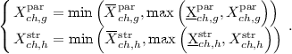 (15)
(15) -
Step 7. Evaluation. In this step all individuals from population \(\mathbf {P'}\) are evaluated according to fitness function (9).
-
Step 8. Merging. This step aim is to select the best N individuals from merged populations \(\mathbf {P}\) and \(\mathbf {P'}\). Selected individuals replace population \(\mathbf {P}\).
-
Step 9. Stopping condition. In this step the stop condition is checked (iteration \( \ge iteration^{\max }\)). If this condition is met, algorithm stops and the best individual according to the fitness function value is presented. Otherwise, the algorithm goes back to Step 3.

 and
and  stand respectively for minims and maxims values of genes
  and
and  stand respectively for minims and maxims values of genes


4 Simulations Results
In our simulations a problem of designing controller structure and tuning parameters for double spring-mass-damp object was considered (see Fig. 3). More details about this model can be found in our previous paper [67]. Object parameters were set as follows: spring constant \(k=10\) N/m, coefficient of friction \(\mu =0.5\), masses \({m_1=m_2=0.2}\) kg. Initial values of: \({s^1}\), \({v^1}\), \({s^2}\) i \({v^2}\) were set to zero, and \(s^*\) is a desired position of mass \(m_1\) (see Fig. 3), simulation length \(T^\mathrm{{all}}\) was set to 10 s, output signal of the controller was limited to the range \(u \in \left( {-2,+2} \right) \), quantization resolution for the output signal y of the controller as well as for the position sensor for \(s^1\) and \(s^2\) was set to 8 bit, time step in the simulation was equal to \(T = 0.1\) ms, while interval between subsequent controller activations were set to twenty simulation steps, number of model iteration is calculated as \(Z={T^\mathrm{{all}}/ T}\). The feedback signals for the controller was chosen as: \(fb_1=s^*\), \(fb_2=s^1\), \(fb_3=s^2\) (\(FB=3\)).

Simulated spring-mass-damp object.
4.1 Problem Evaluation
For problem under consideration a trapezoidal shape of desired signal \(s^*\) was used (see Fig. 4). Moreover, for considered simulation problem, a following fitness function components (9) were used:
-
Complexity of the controller:
$$\begin{aligned} {\mathrm{ffcom}}_1\left( {{{\mathbf{X}}_{ch}}} \right) = \frac{{\sum \limits _{m = 1}^M {\left( {{\mathbf{X}}_{ch}^{{\mathrm{str}} }\left\{ {C_m^{\mathrm{P}}} \right\} + {\mathbf{X}}_{ch}^{{\mathrm{str}} }\left\{ {C_m^{\mathrm{I}}} \right\} + {\mathbf{X}}_{ch}^{{\mathrm{str}} }\left\{ {C_m^{\mathrm{D}}} \right\} + {\mathbf{X}}_{ch}^{{\mathrm{str}} }\left\{ {C_m^{{\mathrm{CB}}}} \right\} } \right) } }}{{4M}}, \end{aligned}$$(16)where notation \({\mathbf{X}}_{ch}^{{\mathrm{str}} }\left\{ a \right\} \) stands for using gene a from chromosome \({\mathbf{X}}_{ch}\).
-
RMSE standing for accuracy of the controlled object:
$$\begin{aligned} \mathrm{{ffcom}_2}\left( \mathbf{{X_{ch}}} \right) = RMSE = \sqrt{\frac{1}{Z}\cdot \sum \limits _{i = 1}^Z {{\varepsilon ^2_{i}}} } = \sqrt{\frac{1}{Z}\cdot \sum \limits _{i = 1}^Z {{{\left( {s_{i}^* - s_{i}^1} \right) }^2}} } , \end{aligned}$$(17) -
Overshooting of the controller:
$$\begin{aligned} \mathrm{{ff}}{\mathrm{{com}}_\mathrm{{3}}}\left( {{\mathbf{{X}}_{\mathbf{{ch}}}}} \right) = \mathop {\max }\limits _{i = 1,...,Z} \left\{ {{s^1_i}} \right\} . \end{aligned}$$(18) -
Oscillations of the output of the controller:
$$\begin{aligned} \mathrm{{ffco}}{\mathrm{{m}}_\mathrm{{4}}}\left( {{\mathbf{{X}}_{\mathbf{{ch}}}}} \right) \mathrm{{ = }}\sum \limits _{\mathrm{{o = 1}}}^{\mathrm{{O - 1}}} {\sqrt{\left| {{\mathrm{{r}}_\mathrm{{o}}}\mathrm{{ - }}{\mathrm{{r}}_{\mathrm{{o + 1}}}}} \right| } } , \end{aligned}$$(19)where \(r_o\) stands for each local minims and maxims of the output values of the controller (those minims and maxims were selected with ignoring noise influence on the signals), \(o=1,...,O\), O stands for number of minims and maxims of osculations.
4.2 Simulation Parameters
In the simulations the following values of parameters were set experimentally: fitness function components weights \(w_1 = 0.1\), \(w_2 = 10\), \(w_3 = 0.01\), \(w_4 = 0.1\), crossover probability \(p_c = 0.75\), mutation probability \(p_m = 0.75\), integer mutation factor \(p_o = 0.50\), number of algorithm iterations \(iteration^{\max }=1000\), number of individuals in populations \(N = 100\).

Best simulations results for: (a) case 0, (b) case 1, (c) case 2, (d) case 3. \(s^1\) stands for position of the mass \(m_1\), \(|s^*-s^1|\) stands for difference with desired position of mass \(m_1\) (\(s^*\)) and \(s^1\), u stands for output of the controller.
4.3 Simulation Cases
In the simulations four cases were tested to show the effectiveness of the proposed controller and learning algorithm:
-
Case 0 - case without filters and noise of the feedback signals (to present possibilities of learning algorithm).
-
Case 1 - case without filters and with 1 % of noise of \(s^1\) and \(s^2\) feedback signals (to show how noise of the signals affect the results).
-
Case 2 - case with filters and with 1 % of noise of \(s^1\) and \(s^2\) feedback signals (to show impact of the filters on the results).
-
Case 3 - case with static filters (\(C^\mathrm{{F}}\) were set to 1) and with 1 % of noise of \(s^1\) and \(s^2\) feedback signals (to show impact of the filters on the results).
For each case simulations were repeat 100 times and results were averaged.
4.4 Obtained Results
The averaged simulations results are presented in Table 1, the best simulations results are presented in Tables 2, 3, Figs. 4 and 5.

Best simulations structures obtained for: (a) case 0, (b) case 1, (c) case 2, (d) case 3. Gray rectangles stands for reduced elements of the controller.
4.5 Simulation Results
Conclusions from the simulation are as follows: (a) including noise of feedback signals significantly degrade the performance of controller (see Fig. 4(a) and (b) and \(\mathrm{{ff}}(\cdot )\) values in Table 1); (b) adding filters allowed us to reduce impact of noise (see Fig. 4(c) and (d) and \(\mathrm{{ff}}(\cdot )\) values in Table 1); (c) using dynamic reduction of filters in learning process (case 2) led to obtain 0.7 (in average) active filters in the controller, which allowed us to obtain 5.6 % accuracy improvement and 7.8 % oscillations improvement of the system (see Fig. 4(b) and (c) and Table 1); (d) using static active filters led to obtain 11.1 % accuracy improvement and 56.6 % oscillations improvement (see Fig. 4(b) and (d) and Table 1); (e) obtained structures are simple and the average reduction of controller elements is close to 50 % (see Fig. 5 and Table 3); (f) the best obtained accuracy of the controller (see Table 2) without noise of feedback signals is better than accuracy obtained by hybrid multi-population algorithms [35]; (g) the best obtained accuracy of the controller (see Table 2) with noise of feedback signals and with use of filters (case 2 and case 3) is close to accuracy obtained by hybrid population algorithms without noise of feedback signals [66].
5 Summary
The proposed elastic structure of the controller containing proposed CB blocks and FIR filters allowed us to obtain accurate and simple controllers, with reduced impact of feedback signals noise on the performance of the controller. Moreover, the proposed training algorithm, which allows reduction of any component of the controller and simultaneously selection of its parameters, allowed us to obtain a very good results in terms of accuracy, superior to the results presented in the literature. In the future, the authors plan to use the proposed controller and learning algorithm in a more complex control problems.
References
Alia, M.A.K., Younes, T.M., Alsabbah, S.A.: A design of a PID self-tuning controller using LabVIEW. J. Softw. Eng. Appl. 4, 161–171 (2011)
Astrom, K.J., Hagglund, T.: PID Controllers: Theory, Design, and Tuning. Instrument Society of America: Research Triangle Park, North Carolina (1995)
Bartczuk, Ł., Rutkowska, D.: Type-2 fuzzy decision trees. In: Rutkowski, L., Tadeusiewicz, R., Zadeh, L.A., Zurada, J.M. (eds.) ICAISC 2008. LNCS (LNAI), vol. 5097, pp. 197–206. Springer, Heidelberg (2008)
Bartczuk, Ł., Rutkowska, D.: Medical diagnosis with type-2 fuzzy decision trees. In: Kkacki, E., Rudnicki, M., Stempczyńska, J. (eds.) Computers in Medical Activity. AISC, vol. 65, pp. 11–21. Springer, Heidelberg (2009)
Bartczuk, Ł., Przybył, A., Dziwiński, P.: Hybrid state variables - fuzzy logic modelling of nonlinear objects. In: Rutkowski, L., Korytkowski, M., Scherer, R., Tadeusiewicz, R., Zadeh, L.A., Zurada, J.M. (eds.) ICAISC 2013, Part I. LNCS, vol. 7894, pp. 227–234. Springer, Heidelberg (2013)
Bartczuk, Ł., Przybył, A., Koprinkova-Hristova, P.: New method for nonlinear fuzzy correction modelling of dynamic objects. In: Rutkowski, L., Korytkowski, M., Scherer, R., Tadeusiewicz, R., Zadeh, L.A., Zurada, J.M. (eds.) ICAISC 2014, Part I. LNCS, vol. 8467, pp. 169–180. Springer, Heidelberg (2014)
Bartczuk, Ł.: Gene expression programming in correction modelling of nonlinear dynamic objects. Adv. Intell. Syst. Comput. 429, 125–134 (2016)
Cpałka, K., Rutkowski, L.: Flexible Takagi-Sugeno fuzzy systems. In: Proceedings of the 2005 IEEE International Joint Conference on Neural Networks, IJCNN 2005, vol. 3, pp. 1764–1769 (2005)
Cpałka, K., Rutkowski, L.: Flexible Takagi-Sugeno neuro-fuzzy structures for nonlinear approximation. WSEAS Trans. Syst. 4(9), 1450–1458 (2005)
Cpalka, K.: A method for designing flexible neuro-fuzzy systems. In: Rutkowski, L., Tadeusiewicz, R., Zadeh, L.A., Żurada, J.M. (eds.) ICAISC 2006. LNCS (LNAI), vol. 4029, pp. 212–219. Springer, Heidelberg (2006)
Cpałka, K., Rutkowski, L.: A new method for designing and reduction of neuro-fuzzy systems. In: Proceedings of the 2006 IEEE International Conference on Fuzzy Systems (IEEE World Congress on Computational Intelligence, WCCI 2006), Vancouver, pp. 8510–8516 (2006)
Cpałka, K.: On evolutionary designing and learning of flexible neuro-fuzzy structures for nonlinear classification. In: Nonlinear Analysis Series A: Theory, Methods and Applications, vol. 71, pp. 1659–1672. Elsevier (2009)
Cpałka, K., Rebrova, O., Nowicki, R., Rutkowski, L.: On design of flexible neuro-fuzzy systems for nonlinear modelling. Int. J. Gen. Syst. 42(6), 706–720 (2013)
Cpałka, K., Łapa, K., Przybył, A., Zalasiński, M.: A new method for designing neuro-fuzzy systems for nonlinear modelling with interpretability aspects. Neurocomputing 135, 203–217 (2014)
Cpałka, K., Zalasiński, M.: On-line signature verification using vertical signature partitioning. Expert Syst. Appl. 41(9), 4170–4180 (2014)
Cpałka, K., Zalasiński, M., Rutkowski, L.: New method for the on-line signature verification based on horizontal partitioning. Pattern Recogn. 47, 2652–2661 (2014)
Cpałka, K., Łapa, K., Przybył, A.: A new approach to design of control systems using genetic programming. Inf. Technol. Control 44(4), 433–442 (2015)
Cpałka, K., Zalasiński, M., Rutkowski, L.: A new algorithm for identity verification based on the analysis of a handwritten dynamic signature. Appl. Soft Comput. (2016, in press). http://dx.doi.org/10.1016/j.asoc.2016.02.017
Duch, W., Korbicz, J., Rutkowski, L., Tadeusiewicz, R. (eds.): Biocybernetics and Biomedical Engineering. Neural Networks, vol. 6. Akademicka Oficyna Wydawnicza EXIT, Warsaw (2000). (in Polish)
Duda, P., Jaworski, M., Pietruczuk, L.: On pre-processing algorithms for data stream. In: Rutkowski, L., Korytkowski, M., Scherer, R., Tadeusiewicz, R., Zadeh, L.A., Zurada, J.M. (eds.) ICAISC 2012, Part II. LNCS, vol. 7268, pp. 56–63. Springer, Heidelberg (2012)
Duda, P., Hayashi, Y., Jaworski, M.: On the strong convergence of the orthogonal series-type kernel regression neural networks in a non-stationary environment. In: Rutkowski, L., Korytkowski, M., Scherer, R., Tadeusiewicz, R., Zadeh, L.A., Zurada, J.M. (eds.) ICAISC 2012, Part I. LNCS, vol. 7267, pp. 47–54. Springer, Heidelberg (2012)
Starczewski, J.T., Bartczuk, Ł., Dziwiński, P., Marvuglia, A.: Learning methods for type-2 FLS based on FCM. In: Rutkowski, L., Scherer, R., Tadeusiewicz, R., Zadeh, L.A., Zurada, J.M. (eds.) ICAISC 2010, Part I. LNCS, vol. 6113, pp. 224–231. Springer, Heidelberg (2010)
Dziwiński, P., Bartczuk, Ł., Przybył, A., Avedyan, E.D.: A new algorithm for identification of significant operating points using swarm intelligence. In: Rutkowski, L., Korytkowski, M., Scherer, R., Tadeusiewicz, R., Zadeh, L.A., Zurada, J.M. (eds.) ICAISC 2014, Part II. LNCS, vol. 8468, pp. 349–362. Springer, Heidelberg (2014)
Dziwiński, P., Avedyan, E.D.: A new approach to nonlinear modeling based on significant operating points detection. In: Rutkowski, L., Korytkowski, M., Scherer, R., Tadeusiewicz, R., Zadeh, L.A., Zurada, J.M. (eds.) ICAISC 2015. LNCS, vol. 9120, pp. 364–378. Springer, Heidelberg (2015)
Er, M.J., Duda, P.: On the weak convergence of the orthogonal series-type kernel regresion neural networks in a non-stationary environment. In: Wyrzykowski, R., Dongarra, J., Karczewski, K., Waśniewski, J. (eds.) PPAM 2011, Part I. LNCS, vol. 7203, pp. 443–450. Springer, Heidelberg (2012)
Gałkowski, T., Rutkowski, L.: Nonparametric recovery of multivariate functions with applications to system identification. Proc. IEEE 73(5), 942–943 (1985)
Roger Jang, J.-S., Sun, C.-T.: Functional equivalence between radial basis function networks and fuzzy inference systems. IEEE Trans. Neural Netw. 4(1), 156–159 (1993)
Jaworski, M., Pietruczuk, L., Duda, P.: On resources optimization in fuzzy clustering of data streams. In: Rutkowski, L., Korytkowski, M., Scherer, R., Tadeusiewicz, R., Zadeh, L.A., Zurada, J.M. (eds.) ICAISC 2012, Part II. LNCS, vol. 7268, pp. 92–99. Springer, Heidelberg (2012)
Kasthurirathna, D., Piraveenan, M., Uddin, S.: Evolutionary stable strategies in networked games: the influence of topology. J. Artif. Intell. Soft Comput. Res. 5(2), 83–95 (2015)
Kinsy, M.A., Majstorovic, D., Haessig, P., Poon J., Celanovic N., Celanovic I., Devadas, S.: High-speed real-time digital emulation for hardware-in-the-loop testing of power electronics: a new paradigm in the field of electronic design automation (EDA) for power electronics systems. In: emphMesago PCIM GmbH, pp. 1–6 (2011)
Korytkowski, M., Rutkowski, L., Scherer, R.: Fast image classification by boosting fuzzy classifiers. Inf. Sci. 327, 175–182 (2016)
Łapa, K., Przybył, A., Cpałka, K.: A new approach to designing interpretable models of dynamic systems. In: Rutkowski, L., Korytkowski, M., Scherer, R., Tadeusiewicz, R., Zadeh, L.A., Zurada, J.M. (eds.) ICAISC 2013, Part II. LNCS, vol. 7895, pp. 523–534. Springer, Heidelberg (2013)
Łapa, K., Zalasiński, M., Cpałka, K.: A new method for designing and complexity reduction of neuro-fuzzy systems for nonlinear modelling. In: Rutkowski, L., Korytkowski, M., Scherer, R., Tadeusiewicz, R., Zadeh, L.A., Zurada, J.M. (eds.) ICAISC 2013, Part I. LNCS, vol. 7894, pp. 329–344. Springer, Heidelberg (2013)
Łapa, K., Cpałka, K., Wang, L.: New method for design of fuzzy systems for nonlinear modelling using different criteria of interpretability. In: Rutkowski, L., Korytkowski, M., Scherer, R., Tadeusiewicz, R., Zadeh, L.A., Zurada, J.M. (eds.) ICAISC 2014, Part I. LNCS, vol. 8467, pp. 217–232. Springer, Heidelberg (2014)
Łapa, K., Szczypta, J., Venkatesan, R.: Aspects of structure and parameters selection of control systems using selected multi-population algorithms. In: Rutkowski, L., Korytkowski, M., Scherer, R., Tadeusiewicz, R., Zadeh, L.A., Zurada, J.M. (eds.) ICAISC 2015. LNCS, vol. 9120, pp. 247–260. Springer, Heidelberg (2015)
Li, X., Er, M.J., Lim, B.S.: Fuzzy regression modeling for tool performance prediction and degradation detection. Int. J. Neural Syst. 20, 405–419 (2010)
Makinana, S., Malumedzha, T., Nelwamondo, F.V.: Quality parameter assessment on iris images. J. Artif. Intell. Soft Comput. Res. 4(1), 21–30 (2014)
Murata, M., Ito, S., Tokuhisa, M., Ma, Q.: Order estimation of Japanese paragraphs by supervised machine learning and various textual features. J. Artif. Intell. Soft Comput. Res. 5(4), 247–255 (2015)
Osowski, S.: Sieci neuronowe w ujkeciu algorytmicznym (in Polish), pp. 160–188. WNT, Warszawa (1996)
Pietruczuk, L., Duda, P., Jaworski, M.: A new fuzzy classifier for data streams. In: Rutkowski, L., Korytkowski, M., Scherer, R., Tadeusiewicz, R., Zadeh, L.A., Zurada, J.M. (eds.) ICAISC 2012, Part I. LNCS, vol. 7267, pp. 318–324. Springer, Heidelberg (2012)
Pietruczuk, L., Zurada, J.M.: Weak convergence of the recursive Parzen-type probabilistic neural network in a non-stationary environment. In: Wyrzykowski, R., Dongarra, J., Karczewski, K., Waśniewski, J. (eds.) PPAM 2011, Part I. LNCS, vol. 7203, pp. 521–529. Springer, Heidelberg (2012)
Jaworski, M., Er, M.J., Pietruczuk, L.: On the application of the Parzen-type kernel regression neural network and order statistics for learning in a non-stationary environment. In: Rutkowski, L., Korytkowski, M., Scherer, R., Tadeusiewicz, R., Zadeh, L.A., Zurada, J.M. (eds.) ICAISC 2012, Part I. LNCS, vol. 7267, pp. 90–98. Springer, Heidelberg (2012)
Pietruczuk, L., Duda, P., Jaworski, M.: Adaptation of decision trees for handling concept drift. In: Rutkowski, L., Korytkowski, M., Scherer, R., Tadeusiewicz, R., Zadeh, L.A., Zurada, J.M. (eds.) ICAISC 2013, Part I. LNCS, vol. 7894, pp. 459–473. Springer, Heidelberg (2013)
Przybyl, A., Smolkag, J., Kimla, P.: Distributed control system based on real time ethernet for computer numerical controlled machine tool (in Polish). Przeglad Elektrotechniczny 86(2), 342–346 (2010)
Przybył, A., Cpałka, K.: A new method to construct of interpretable models of dynamic systems. In: Rutkowski, L., Korytkowski, M., Scherer, R., Tadeusiewicz, R., Zadeh, L.A., Zurada, J.M. (eds.) ICAISC 2012, Part II. LNCS, vol. 7268, pp. 697–705. Springer, Heidelberg (2012)
Przybył, A., Er, M.J.: The idea for the integration of neuro-fuzzy hardware emulators with real-time network. In: Rutkowski, L., Korytkowski, M., Scherer, R., Tadeusiewicz, R., Zadeh, L.A., Zurada, J.M. (eds.) ICAISC 2014, Part I. LNCS, vol. 8467, pp. 279–294. Springer, Heidelberg (2014)
Przybył, A., Szczypta, J., Wang, L.: Optimization of controller structure using evolutionary algorithm. In: Rutkowski, L., Korytkowski, M., Scherer, R., Tadeusiewicz, R., Zadeh, L.A., Zurada, J.M. (eds.) Artificial Intelligence and Soft Computing. LNCS, vol. 9120, pp. 261–271. Springer, Heidelberg (2015)
Rutkowski, L.: Sequential estimates of probability densities by orthogonal series and their application in pattern classification. IEEE Trans. Syst. Man Cybern. 10(12), 918–920 (1980)
Rutkowski, L.: Nonparametric identification of quasi-stationary systems. Syst. Control Lett. 6(1), 33–35 (1985)
Rutkowski, L.: Real-time identification of time-varying systems by non-parametric algorithms based on Parzen kernels. Int. J. Syst. Sci. 16(9), 1123–1130 (1985)
Rutkowski, L.: A general approach for nonparametric fitting of functions and their derivatives with applications to linear circuits identification. IEEE Trans. Circ. Syst. 33(8), 812–818 (1986)
Rutkowski, L.: Application of multiple Fourier-series to identification of multivariable non-stationary systems. Int. J. Syst. Sci. 20(10), 1993–2002 (1989)
Rutkowski, L., Cpałka, K.: Flexible structures of neuro-fuzzy systems. In: Sincak, P., Vascak, J. (eds.) Quo Vadis Computational Intelligence. Studies in Fuzziness and Soft Computing, vol. 54, pp. 479–484. Springer, Heidelberg (2000)
Rutkowski, L., Cpałka, K.: Compromise approach to neuro-fuzzy systems. In: Sincak, P., Vascak, J., Kvasnicka, V., Pospichal, J. (eds.) Intelligent Technologies - Theory and Applications, vol. 76, pp. 85–90. IOS Press (2002)
Rutkowski, L.: Computational Intelligence. Springer, Heidelberg (2008)
Rutkowski, L.: Adaptive probabilistic neural networks for pattern classification in time-varying environment. IEEE Trans. Neural Netw. 15(4), 811–827 (2004)
Rutkowski, L., Przybył, A., Cpałka, K., Er, M.J.: Online speed profile generation for industrial machine tool based on neuro-fuzzy approach. In: Rutkowski, L., Scherer, R., Tadeusiewicz, R., Zadeh, L.A., Zurada, J.M. (eds.) ICAISC 2010, Part II. LNCS, vol. 6114, pp. 645–650. Springer, Heidelberg (2010)
Rutkowski, L., Przybył, A., Cpałka, K.: Novel online speed profile generation for industrial machine tool based on flexible neuro-fuzzy approximation. IEEE Trans. Industr. Electron. 59(2), 1238–1247 (2012)
Rutkowski, L., Pietruczuk, L., Duda, P., Jaworski, M.: Decision trees for mining data streams based on the McDiarmid’s bound. IEEE Trans. Knowl. Data Eng. 25(6), 1272–1279 (2013)
Rutkowski, L., Jaworski, M., Pietruczuk, L., Duda, P.: Decision trees for mining data streams based on the Gaussian approximation. IEEE Trans. Knowl. Data Eng. 26(1), 108–119 (2014)
Rutkowski, L., Jaworski, M., Pietruczuk, L., Duda, P.: The CART decision tree for mining data streams. Inf. Sci. 266, 1–15 (2014)
Rutkowski, L., Jaworski, M., Pietruczuk, L., Duda, P.: A new method for data stream mining based on the misclassification error. IEEE Trans. Neural Netw. Learn. Syst. 26(5), 1048–1059 (2015)
Starczewski, J.T., Rutkowski, L.: Connectionist structures of type 2 fuzzy inference systems. In: Wyrzykowski, R., Dongarra, J., Paprzycki, M., Waśniewski, J. (eds.) PPAM 2001. LNCS, vol. 2328, pp. 634–642. Springer, Heidelberg (2002)
Starczewski, J., Rutkowski, L.: Interval type 2 neuro-fuzzy systems based on interval consequents. In: Rutkowski, L., Kacprzyk, J. (eds.) Neural Networks and Soft Computing, pp. 570–577. Physica-Verlag, New York (2003). A Springer-Verlag Company, Heidelberg
Schulte, T., Kiffe, A., Puschmann, F.: HIL simulation of power electronics and electric drives for automotive applications. emphElectronics 16(2), 130–135 (2012)
Szczypta, J., Łapa, K., Shao, Z.: Aspects of the selection of the structure and parameters of controllers using selected population based algorithms. In: Rutkowski, L., Korytkowski, M., Scherer, R., Tadeusiewicz, R., Zadeh, L.A., Zurada, J.M. (eds.) ICAISC 2014, Part I. LNCS, vol. 8467, pp. 440–454. Springer, Heidelberg (2014)
Szczypta, J., Przybył, A., Cpałka, K.: Some aspects of evolutionary designing optimal controllers. In: Rutkowski, L., Korytkowski, M., Scherer, R., Tadeusiewicz, R., Zadeh, L.A., Zurada, J.M. (eds.) ICAISC 2013, Part II. LNCS, vol. 7895, pp. 91–100. Springer, Heidelberg (2013)
Zalasiński, M., Cpałka, K.: Novel algorithm for the on-line signature verification. In: Rutkowski, L., Korytkowski, M., Scherer, R., Tadeusiewicz, R., Zadeh, L.A., Zurada, J.M. (eds.) ICAISC 2012, Part II. LNCS, vol. 7268, pp. 362–367. Springer, Heidelberg (2012)
Zalasiński, M., Cpałka, K.: Novel algorithm for the on-line signature verification using selected discretization points groups. In: Rutkowski, L., Korytkowski, M., Scherer, R., Tadeusiewicz, R., Zadeh, L.A., Zurada, J.M. (eds.) ICAISC 2013, Part I. LNCS, vol. 7894, pp. 493–502. Springer, Heidelberg (2013)
Zalasiński, M., Łapa, K., Cpałka, K.: New algorithm for evolutionary selection of the dynamic signature global features. In: Rutkowski, L., Korytkowski, M., Scherer, R., Tadeusiewicz, R., Zadeh, L.A., Zurada, J.M. (eds.) ICAISC 2013, Part II. LNCS, vol. 7895, pp. 113–121. Springer, Heidelberg (2013)
Zalasiński, M., Cpałka, K., Er, M.J.: New method for dynamic signature verification using hybrid partitioning. In: Rutkowski, L., Korytkowski, M., Scherer, R., Tadeusiewicz, R., Zadeh, L.A., Zurada, J.M. (eds.) ICAISC 2014, Part II. LNCS, vol. 8468, pp. 216–230. Springer, Heidelberg (2014)
Zalasiński, M., Cpałka, K., Hayashi, Y.: New method for dynamic signature verification based on global features. In: Rutkowski, L., Korytkowski, M., Scherer, R., Tadeusiewicz, R., Zadeh, L.A., Zurada, J.M. (eds.) ICAISC 2014, Part II. LNCS, vol. 8468, pp. 231–245. Springer, Heidelberg (2014)
Zalasiński, M., Cpałka, K., Er, M.J.: A new method for the dynamic signature verification based on the stable partitions of the signature. In: Rutkowski, L., Korytkowski, M., Scherer, R., Tadeusiewicz, R., Zadeh, L.A., Zurada, J.M. (eds.) ICAISC 2015. LNCS, vol. 9120, pp. 161–174. Springer, Heidelberg (2015)
Zalasiński, M., Cpałka, K., Hayashi, Y.: New fast algorithm for the dynamic signature verification using global features values. In: Rutkowski, L., Korytkowski, M., Scherer, R., Tadeusiewicz, R., Zadeh, L.A., Zurada, J.M. (eds.) ICAISC 2015. LNCS, vol. 9120, pp. 175–188. Springer, Heidelberg (2015)
Acknowledgment
The project was financed by the National Science Center (Poland) on the basis of the decision number DEC-2012/05/B/ST7/02138.
Author information
Authors and Affiliations
Corresponding author
Editor information
Editors and Affiliations
Rights and permissions
Copyright information
© 2016 Springer International Publishing Switzerland
About this paper
Cite this paper
Przybył, A., Łapa, K., Szczypta, J., Wang, L. (2016). The Method of the Evolutionary Designing the Elastic Controller Structure. In: Rutkowski, L., Korytkowski, M., Scherer, R., Tadeusiewicz, R., Zadeh, L., Zurada, J. (eds) Artificial Intelligence and Soft Computing. ICAISC 2016. Lecture Notes in Computer Science(), vol 9692. Springer, Cham. https://doi.org/10.1007/978-3-319-39378-0_41
Download citation
DOI: https://doi.org/10.1007/978-3-319-39378-0_41
Published:
Publisher Name: Springer, Cham
Print ISBN: 978-3-319-39377-3
Online ISBN: 978-3-319-39378-0
eBook Packages: Computer ScienceComputer Science (R0)