
Abstract
A minimal models of vertebrae formation were studied in concerning periodic structures formation. The authors proposed two kinds of reaction-diffusion models, from which one is of clock-and-wavefront type and the other one is of Turing type. Our goal is to show that in case of the Turing type model the kinetic system as well the reaction-diffusion system exhibit oscillating solutions. The chapter is organised as follows. In the next section we introduce the model. In the section that follows we examine the existence and stability of some equilibria. In the third section we show the occurence of Hopf bifurcation in the kinetic system as well as in the parabolic system.
Access provided by Autonomous University of Puebla. Download chapter PDF
1 Introduction
A minimal models of vertebrae formation were studied in [8] concerning periodic structures formation. The authors proposed two kinds of reaction-diffusion models, from which one is of clock-and-wavefront type and the other one is of Turing type. Our goal is to show that in case of the Turing type model the kinetic system as well the reaction-diffusion system exhibit oscillating solutions. The chapter is organised as follows. In the next section we introduce the model. In the section that follows we examine the existence and stability of some equilibria. In the third section we show the occurence of Hopf bifurcation in the kinetic system as well as in the parabolic system.
2 The Model
The model proposed by Annie Lemarchand and Bogdan Nowakowski (cf. [8]), which describes vertebrae formation is governed by
on \(\overline {\Omega }\times \mathbb {R}_0^+\) where Ω is a bounded, connected spatial domain with piecewise smooth boundary ∂ Ω, d A, d B > 0 represent the diffusion coefficients, A(r, t) and B(r, t) are the concentrations of the species at time t ∈ [0, +∞) and place \(\mathbf {r}\in \overline {\Omega }\). The kinetic part of the model (1)
(α, β, γ, δ > 0) was inspired from the Schnakenberg model (cf. [9])
and the Gray-Schott model (cf. [4])
We are interested in solutions \(\boldsymbol {\Phi }:\overline {\Omega } \times \mathbb {R}^+_0\rightarrow \mathbb {R}^2\) of (2) that satisfy the no-flux boundary conditions
resp. non-negative initial conditions
where S := (A, B), and n denotes the outer unit normal to ∂ Ω.
3 The Kinetic System
It was mentioned in the original paper [8] that parameters α, β, γ, δ are chosen such that the system possesses three steady states. It is easy to see that this is the case when
holds. In this case the kinetic system (2) exhibits three equilibria in the first quadrant of the phase space, namely one on the boundary: E b := (0, γ∕δ) and two interior equilibria (cf. Fig. 1.): E ± := (A ∓, B ±) where

A phase portrait of system (2) for K < 0, resp. K > 0
In what follows we study the stability of possible equilibria \(\overline {\mathbf {S}}:=(\overline {S}_1,\overline {S}_2)\) of the kinetic system (2) and the possibility of Hopf bifurcations. The coefficient matrix of the system linearized at \(\overline {\mathbf {S}}\) is
with trace

and determinant
A simple linear stability analysis shows that E b is always locally asymptotically stable, because the Jacobian of system (2) at these equilibrium point takes the form
The Jacobians evaluated at E ± have the form
and
Based on the form of the characteristic polynomial

it is easy to determine the stability of the equilibrium points. It is clear that
-
the matrix J + is unstable, because
and
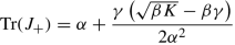
$$\displaystyle \begin{aligned}\det(J_+)=\frac{K-\gamma\sqrt{\beta K}}{2\alpha}, \end{aligned}$$furthermore \(\det (J_+)\) is negative due to K < βγ 2;
-
the matrix J − is stable if and only if
hold, because
$$\displaystyle \begin{aligned}\det(J_-)=\frac{K+\gamma\sqrt{\beta K}}{2\alpha}>0. \end{aligned}$$


Since the determinant of J
− stays positive, then Hopf bifurcation can occur only if the trace is changing its sign. It is easy to calculate that if α > δ then  if and only if
holds. Thus, by fixed α, γ, δ, the parameter β will play the role of the bifurcating parameter.
Theorem 3.1
Suppose that
hold, then at
the equilibrium E −(β) of (2) undergoes a Poincaré-Andronov-Hopf bifurcation: E −(β) loses its stability at β ∗ and system (2) has a branch of periodic solutions bifurcating from E −(β) near β = β ∗ (cf. Fig. 2 .).

Proof
The characteristic polynomial of the matrix \(\mathfrak {A}\) at E −(β) has the form

where

Clearly,
resp. from (8)

follows, which proves the statements of the theorem (cf. [5, 7]). □
4 The Parabolic System
In what follows we consider system (1) with homogeneous Neumann boundary conditions (5) and nonnegative initial conditions (6). Clearly, a spatially constant solution Φ(⋅) = ( Φ1(⋅), Φ2(⋅)) of system (1) satisfies boundary conditions (5) and system (2). The equilibria of system (2) are constant solutions of (1), (5) at the same time. In order to investigate the local dynamical behavior of system (1) near the equilibria E b and E ± of (2) we linearize (1) at these equilibria. The linearized system at the equilibrium point
with the same initial and boundary conditions has the form
where
Using the method of eigenfunction expansions for the spatial domain Ω the solutions of problem (10) and (11) have the form
(cf. [6]), where for \(n\in \mathbb {N}_0\)
and λ n is the nth eigenvalue of the minus Laplacian on Ω subject to homogeneous Neumann boundary conditions, resp. ψ n is the corresponding normalized eigenfunction, i.e. λ n and ψ n are solutions of
It is well known (cf. [3]) that
and the eigenfunctions to different eigenvalues are orthogonal to each other.
According to [1, 2] the equilibrium S of (1), (5) is asymptotically stable if for all \(n\in \mathbb {N}_0\) the matrix \(\mathfrak {A}_n\) is stable, i.e. both eigenvalues of \(\mathfrak {A}_n\) have negative real parts; furthermore S is unstable if for some index \(n\in \mathbb {N}_0\) there exists an eigenvalue of \(\mathfrak {A}_n\) with positive real part. The characteristic polynomial of the matrix \(\mathfrak {A}_n\) have the form
where

and
Thus, if S = (S 1, S 2) = E − then for all β > 0 the characteristic equation of \(\mathfrak {A}_n\) has the form
where
and
In order to have Hopf bifurcation one has to show that a pair of complex conjugate roots
crosses the imaginary axis with non-zero velocity, that is for a β ∗ > 0
hold. This is fulfilled (cf. [5]) if exists \(n\in \mathbb {N}_0\) and β ∗ > 0 such that
and
We have to remark that β ∗ in (9) is always a Hopf bifurcation value, since
resp.
if
hold. This corresponds to the Hopf bifurcation of spatially homogeneous periodic orbits which have been known from Theorem 3.1. Apparently β ∗ is also the unique value for β for the Hopf bifurcation of spatially homogeneous periodic orbits (cf. Fig. 3.).

In what follows, we shall search for spatially non-homogeneous Hopf bifurcation value in case of \(n\in \mathbb {N}\). For \(0\leq \beta \in \mathbb {R}\) let define
then
and it follows from (7) that
This means that E is stricktly decreasing and in case of
there is a unique solution β = β n > 0 of the equation
Direct calculation shows that the unique positive solution has the form
holds.
Theorem 4.1
The transversality condition, i.e.
is satisfied.
Proof
It is easy to see that
which proves the statement of the theorem. □
It is also clear that for all \(n\in \mathbb {N}\)
hold.
Next we will investigate whether
and in particular, \(\mathfrak {D}_n(\beta _n)>0\). It is easy to see that
Because
where
and
we obtain the following result.
Theorem 4.2
If an \(n\in \mathbb {N}_0\) is chosen such that assumptions (17) and
hold, then in system (1) Poincaré-Andronov-Hopf bifurcation takes place: E −(β) loses its stability at β n and system (1) has a branch of periodic solutions bifurcating from E −(β) near β = β n.
Proof
Obviously, if (17) holds then
Thus,
Hence, if condition (19) holds then
This means that \(\mathfrak {D}_m(\beta _n)>0\). This with the transversality condition (18) together proves Hopf bifurcation. □
References
Britton, N. F.: Reaction-diffusion equations and their applications to biology. Academic Press, Inc., London, 1986.
Casten, Richard G.; Holland, Charles J.: Stability properties of solutions to systems of reaction-diffusion equations, SIAM J. Appl. Math., 33(2) (1977), 353–364.
Evans, L. C.: Partial differential equations, Second edition. Graduate Studies in Mathematics, 19. American Mathematical Society, Providence, RI, 2010.
Gray, P.; Scott, S. K.: Autocatalytic reactions in the isothermal continuous stirred tank reactor: oscillations and instabilities in the system A + 2B → 3B; B → C, Chem. Eng. Sci., 39 (1984), 1087–1097.
Hassard, B. D.; Kazarinoff, N. D.; Wan, Y. H.: Theory and applications of Hopf bifurcation, London Mathematical Society Lecture Note Series, 41. Cambridge University Press, Cambridge-New York, 1981.
Kovács, S.: Turing bifurcation in a system with cross diffusion, Nonlinear Anal., 59(4) (2004), 567–581.
Kovács, S.; György, S.Z.; Gyúró, N.: On an Invasive Species Model with Harvesting, in: Trends in Biomathematics: Modeling Cells, Flows, Epidemics, and the Environment (ed. R. Mondaini), (Springer 2020), 299–334.
Lemarchand, A.; Nowakowski, B.: Do the internal fluctuations blur or enhance axial segmentation?, EPL, 94 (2011) 48004.
Schnakenberg, J.: Simple chemical reaction systems with limit cycle behaviour, J. Theoret. Biol. , 81(3) (1979), 389–400.
Acknowledgements
The authors were supported in part by the European Union, co-financed by the European Social Fund (EFOP-3.6.3-VEKOP-16-2017-00001).
Author information
Authors and Affiliations
Corresponding author
Editor information
Editors and Affiliations
Rights and permissions
Copyright information
© 2022 The Author(s), under exclusive license to Springer Nature Switzerland AG
About this chapter

Cite this chapter
Kovács, S., György, S., Gyúró, N. (2022). Oscillations in a System Modelling Somite Formation. In: Mondaini, R.P. (eds) Trends in Biomathematics: Stability and Oscillations in Environmental, Social, and Biological Models. BIOMAT 2021. Springer, Cham. https://doi.org/10.1007/978-3-031-12515-7_13
Download citation
DOI: https://doi.org/10.1007/978-3-031-12515-7_13
Published:
Publisher Name: Springer, Cham
Print ISBN: 978-3-031-12514-0
Online ISBN: 978-3-031-12515-7
eBook Packages: Mathematics and StatisticsMathematics and Statistics (R0)