Sequentialising Nested Systems

Abstract

In this work, we investigate the proof theoretic connections between sequent and nested proof calculi. Specifically, we identify general conditions under which a nested calculus can be transformed into a sequent calculus by restructuring the nested sequent derivation (proof) and shedding extraneous information to obtain a derivation of the same formula in the sequent calculus. These results are formulated generally so that they apply to calculi for intuitionistic, normal modal logics and negative modalities.

Funded by the project Reasoning Tools for Deontic Logic and Applications to Indian Sacred Texts, CAPES, CNPq, START, FWF-ANR and TICAMORE (I 2982).

1 Introduction

Contemporary proof theory can be traced to Gentzen’s seminal work [8] where analytic proof calculi for classical and intuitionistic logic were presented. Proof calculi consist of formal rules of inference which describe the logic under consideration; in an analytic calculus, every formula that occurs in a proof generated by the calculus is a subformula of the end formula being proved. Analyticity is crucial because it induces a structure on the proofs (in terms of the end formula). This proof structure can be exploited to formalise reasoning, investigate metalogical properties of the logic e.g. decidability, complexity and interpolation, and develop automated deduction procedures.

The wide applicability of logical methods and their use in new subject areas has resulted in an explosion of new logics different from classical logic; their usefulness depends on the availability of an analytic proof calculus. The sequent calculus is the simplest and best-known formalism for constructing analytic proof calculi. Unfortunately, there are many natural non-classical logics—for example, most extensions of intuitionistic and modal logic—for which the sequent calculus formalism is unable to provide an analytic calculus (the precise reasons for this inability are still not well understood). In response, many more new formalisms have been proposed, such as hypersequents [2, 21], labelled sequents [6, 18], nested sequents [3, 10] and linear nested sequents [14, 16]. This work is primarily concerned with the nested sequent formalism which is obtained by replacing the sequent in the sequent calculus with a tree of sequents.

While the trend has been towards developing formalisms with greater sophistication in order to provide non-classical logics with analytic calculi, in this work we look in the reverse direction by investigating which aspects of this sophistication are extraneous. More specifically, we identify general conditions under which a nested calculus can be transformed into a sequent calculus by restructuring the nested sequent derivation (proof) and shedding information to obtain a derivation of the same formula in the sequent calculus. Our approach identifies a class of nested systems, called basic nested systems, suitable for such transformations. In these systems, nested rules either create new nestings (creation rules), or manage sequent contexts (update rules), moving formulae to deeper nestings, with nesting depth difference exactly equal to one. This builds an interesting connection with Avron and Lahav’s basic sequent systems [1, 11], since the systematic separation of the behaviour of principal-auxiliary/context formulae in basic sequent systems and creation/update rules allows for a neater way of relating sequent and nested frameworks.

We exploit this separation of rules as follows: after creating a new nesting, upgrade rules control the flow of formulas from the surrounding context to nestings. We show that, if this flow is restricted to stepwise, (bottom-up) outside-in moves, then the whole block of applications of nested rules can be seen as a single sequent rule, with the principal and auxiliary formulae determined by the creation rule, and the context restrictions determined by the upgrade rules. Observe that the proof strategy described above is only possible since basic nested systems allow for a general form of the disjunction property. We apply this method to intuitionistic, normal modal logics and negative modalities.

We believe that the material presented here is not only a mere technicality for establishing connections between proof formalisms: on pinpointing the key differences between sequent and nested systems, we are in fact shedding some light on the discussion of to what extent sequent calculus is an adequate meta-language for producing analytic systems. We thus finish the paper by showing how our ideas can be used in order to better understand the bounds for analyticity in sequent systems.

Organisation and Contributions. Section 2 presents the notation for basic sequent systems; Sect. 3 introduces the notion of basic nested systems and shows a normalisation procedure for nested sequent derivations; Sect. 4 explains how to recover sequent systems from nested ones; Sect. 5 applies our results to some example logics and brings a discussion about nestings and cut-elimination; Sect. 6 concludes the paper.

2 Sequent Systems

In [1] a family of sequent systems (called basic systems) was uniformly presented by explicitly differentiating the context and non-context portions of a rule. The former is defined using binary context relations and the latter via a specified rigid structure. The advantage of such a presentation is that it allows us to relate the properties of the rule with the formal specification of its content and non-context. We will greatly explore this separation when relating sequent rule applications to blocks of nested derivations in Sect. 4. In this work, we will adopt the presentation for basic systems given in [11]. Where convenient, we will also present sequent systems using the traditional rule schemas built from meta-variables for formulae and sets of formulae.

Let $\mathcal {L}$ denote a propositional language and the set of its well formed formulae, built using a countable set of propositional variable symbols.

Definition 1

A signed formula is an expression of the form $\mathsf {T}:A$ or $\mathsf {F}:A$ where . A sequent is a finite set of signed formulae. As in [11], we will adopt the usual sequent notation $\varGamma \vdash \varDelta$, where $\varGamma ,\varDelta$ are (possibly empty) finite sets of formulae and $\varGamma \vdash \varDelta$ is interpreted as the sequent $\{\mathsf {F}:A \mid A\in \varGamma \} \cup \{\mathsf {T}:A \mid A\in \varDelta \}$.

A substitution is a function such that

$$\sigma (\heartsuit (A_1,\ldots ,A_k))=\heartsuit (\sigma (A_1),\ldots ,\sigma (A_k))$$

for every k-ary connective $\heartsuit$ of $\mathcal {L}$. Substitutions extend to signed formulae (preserving sign), sequents and (later) to nested sequents in the standard way.

A context relation is a finite binary relation on the set of signed formulae. Given a context relation $\mathcal {C}$, we denote by $\overline{\mathcal {C}}$ the binary relation between signed formulae $\overline{\mathcal{C}}=\{\langle \sigma (\alpha ),\sigma (\beta ) \rangle \mid \sigma$ is a substitution, and $\langle \alpha ,\beta \rangle \in \mathcal{C}\}$.

A $\mathcal{C}$-instance is a pair of sequents $\langle S_1,S_2 \rangle$ such that for some enumeration $S_1 = \{\alpha _1,\ldots ,\alpha _k\}$ and $S_2 = \{\beta _1,\ldots ,\beta _k\}$ and every $1\le i \le k$, it is the case that $\alpha _i\overline{\mathcal{C}}\beta _i$.

Example 2

From the trivial relation $\mathcal {C}_{\mathtt {id}} := \{\langle \mathsf {F}:p,\mathsf {F}:p \rangle ,\langle \mathsf {T}:p,\mathsf {T}:p \rangle \}$ it follows that a signed formula is $\overline{\mathcal{C}}_{\mathtt {id}}$-related to another iff the two signed formulae are identical. It follows that the $\mathcal {C}_{\mathtt {id}}$-instances are precisely the sets $\{ \langle S,S \rangle \mid \text {S is a sequent} \}$ of pairs.

From the relation $\mathcal {C}_{\mathsf {int}} := \{\langle \mathsf {F}:p,\mathsf {F}:p \rangle \}$ it follows that while $(\mathsf {F}:A)\overline{\mathcal{C}}_{\mathsf {int}} (\mathsf {F}:A)$ for every formula A, it is not the case that $(\mathsf {T}:A)\overline{\mathcal{C}}_{\mathsf {int}} (\mathsf {T}:A)$. In particular, the $\mathcal {C}_{\mathsf {int}}$-instances are precisely those sequent pairs of the form $\langle \varGamma \vdash ,\varGamma \vdash \rangle$. Informally, $\mathcal {C}_{\mathsf {int}}$-instances are identical sequents with empty right hand side.

Let $\Box \varGamma$ denote the set $\{\Box A\mid A\in \varGamma \}$. Then from $\mathcal {C}_{\mathsf {K}} := \{\langle \mathsf {F}:p,\mathsf {F}:\Box p \rangle \}$ it follows that $\mathcal {C}_{\mathsf {K}}$-instances are precisely those sequent pairs of the form $\langle \varGamma \vdash ,\Box \varGamma \vdash \rangle$.

Finally, from the relation $\mathcal {C}_{\mathsf {4}} := \{\langle \mathsf {F}:\Box p,\mathsf {F}:\Box p \rangle \}$ it follows that $\mathcal {C}_{\mathsf {4}}$-instances are precisely those sequent pairs of the form $\langle \Box \varGamma \vdash ,\Box \varGamma \vdash \rangle$.

We define the concatenation $(\varGamma _1\vdash \varDelta _1)\otimes (\varGamma _2\vdash \varDelta _2)$ as $\varGamma _1,\varGamma _2\vdash \varDelta _1,\varDelta _2$, and $\emptyset \otimes \varPi$ as $\emptyset$.

Definition 3

A basic premise is a pair $\langle S;\mathcal {C}\rangle$ where S is a sequent and $\mathcal {C}$ is a context relation. A basic rule is a pair $s{/}S$ where $s=\{\langle S_i;\mathcal {C}_{i}\rangle \}_{1\le i\le k}$ is a finite set of basic premises and S is the conclusion sequent of the rule. A basic rule is represented explicitly as:

The formulae in $S_{i}$ ($1\le i\le k$) are called auxiliary formulae and the formulae in S are called the principal formulae.

A rule with an empty set of basic premises is called an axiom. A basic sequent system ($\mathsf {SC}$) consists of a set of basic rules.

An application of a basic rule has the following form, where $\sigma$ is a substitution, $\varPi _{1},\varPi _{1}',\ldots ,\varPi _{k},\varPi _{k}'$ are sequents and $\langle \varPi _i,\varPi '_i \rangle$ is a $\mathcal{C}_i$-instance for each i ($1\le i\le k$).

The notion of premise, conclusion, principal and auxiliary formulae extends to applications of rules in the standard way.

A derivation in a $\mathsf {SC}$ is defined in the usual way as a finite labelled rooted tree: the root is labelled by the end-sequent, the labels of each node and its children correspond to the conclusion and premises of a rule application, and axioms label the leaves.

Fig. 1.

Multi-conclusion intuitionistic calculus $\mathsf {SC}_\mathsf {mLJ}$.

Example 4

The rule below on the left has principal formula $p_1\rightarrow p_2$, auxiliary formulae $p_1,p_2$, and application depicted on the right

Example 5

The axiom $\mathsf {init}$, and the right and left weakening rules are defined as follows:

$$ \emptyset /p\vdash p\qquad \qquad \langle \emptyset ;\mathcal {C}_\mathtt {id}\rangle /\vdash p \qquad \qquad \langle \emptyset ;\mathcal {C}_\mathtt {id}\rangle /p\vdash $$

In the presence of the above rules, the following rules can be seen to be derivable:

Remark 6

The systems that we consider will be fully structural in the sense that free application of the schemas $\mathsf {init}$ and $\mathsf {W}$ is permitted (as originally in the definition of basic sequent systems in [11]). Observe that, since sequents are sets, we do not the copy formulae in the contexts.

Figure 1 presents (the schema representation of) $\mathsf {SC}_\mathsf {mLJ}$ [17], a multiple conclusion sequent system for propositional intuitionistic logic. Observe that all rules, except $\rightarrow _R$, have the trivial relation in the basic premises. On the other hand, the relation $\mathcal {C}_\mathsf {int}$ in the implication right rule enforces that the only formula in the succedent of the conclusion is the principal formula.

In what follows, for readability, we may omit the word basic when referring to rules, applications and systems.

3 Nested Systems

Nested systems [4, 20] are extensions of the sequent framework where each sequent is replaced by a tree of sequents. In this work, we will identify a family of basic nested systems, inspired by [1, 13].

Definition 7

A nested sequent is defined inductively as follows:

• (i) if S is a sequent, then it is a nested sequent;

• (ii) if $\varGamma \vdash \varDelta$ is a sequent and $G_1,\ldots ,G_k$ are nested sequents, then $\varGamma \vdash \varDelta ,\left[ G_1\right] ,\ldots ,\left[ G_k\right]$ is a nested sequent.

A nested rule is a pair $\upsilon /\varUpsilon$ represented as follows, where $\upsilon =\{\varUpsilon _1,\ldots ,\varUpsilon _k\}$ is a finite set of nested sequents (the premises) and $\varUpsilon$ is the conclusion nested sequent of the rule.

The non-context formulae in the premises are called auxiliary formulae and the non-context formulae in the conclusion are called principal formulae.

For a sequent $S=\varGamma \vdash \varDelta$, define $S\otimes (\vdash \left[ \vdash \right] )$ to be the nested sequent $\varGamma \vdash \varDelta ,\left[ \vdash \right]$.

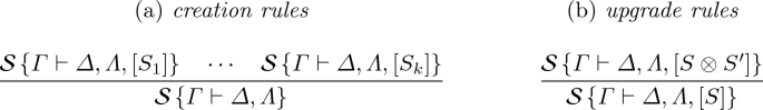
Let $S,S_{1},\ldots ,S_{k}$ be sequents. A basic nested rule has one of the following forms:

• i. sequent-like rules

  

• ii. nested-like rules

  

  *Upgrade rules must have exactly one principal and auxiliary formulae.

We will call the nestings in the premises of a creation rule its auxiliary nestings. Nestings containing principal or auxiliary formulae are called active.

Example 8

Consider the following nested-like rules

The first is a creation rule, with auxiliary nesting $\left[ p_1\vdash p_2\right]$; the second an upgrade rule.

Remark 9

Observe that our definition of nested-like rules restricts the rule form in three ways. First, nested-like rules must have exactly one nesting in the premises or conclusion. Second, information in nested rules always moves deeper inside nestings, when reading rules bottom-up. Finally, upgrade rules move only one piece of information at a time. The first restriction is crucial for avoiding non-determinism when defining of applications of rules; the second one will be key for stating sufficient conditions for the linearisation of nested systems; the third restriction is natural but not necessary. In fact, nested rules usually are local, acting in one formula at a time. Also, upgrade rules naturally have this shape, which will allow for the identification of upgrade nested rules as basic sequent context relations later in Sect. 4.

We will present, in Sect. 5, some examples of basic nested systems. It is worth mentioning that every nested calculus we know that has a correspondence (in the sense of this paper) with sequent systems is equivalent to a basic nested system. On the other hand, the restrictions above exclude, e.g., the representation of the rules for modal axioms $\mathsf {5}$ and $\mathsf {B}$ [4]. But then, there are no known simple, cut-free sequent systems for logics $\mathsf {K}\mathsf {5}$ and $\mathsf {K}\mathsf {B}$. We will discuss some cases that fall outside our scope also in Sect. 5.

For readability, we will denote by $\varGamma ,\varDelta$ sequent contexts and by $\varLambda$ sets of nestings. In this way, every nested sequent has the shape $\varGamma \vdash \varDelta , \varLambda$ where elements of $\varLambda$ have the shape $[\varGamma '\vdash \varDelta ', \varLambda ']$ and so on. We will denote by $\varUpsilon$ arbitrary nested sequents. Application of rules and schemas in nested systems will be represented using holed contexts.¹

Definition 10

A nested-holed context is a nested sequent that contains a hole of the form $\{ \; \}$ in place of nestings. We represent such a context as $\mathcal {S}\left\{ \;\right\}$. Given a holed context and a nested sequent $\varUpsilon$, we write $\mathcal {S}\left\{ \varUpsilon \right\}$ to stand for the nested sequent where the hole $\{\;\}$ has been replaced by $\left[ \varUpsilon \right]$, assuming that the hole is removed if $\varUpsilon$ is empty and if $\mathcal {S}$ is empty then $\mathcal {S}\left\{ \varUpsilon \right\} =\varUpsilon$.

For example, $(\varGamma \vdash \varDelta ,\{\;\})\{\varGamma '\vdash \varDelta '\}= \varGamma \vdash \varDelta ,\left[ \varGamma '\vdash \varDelta '\right]$ while $\{\;\}\{\varGamma '\vdash \varDelta '\}= \varGamma '\vdash \varDelta '$ and $(\varGamma \vdash \varDelta ,\{\;\})\{\;\}= \varGamma \vdash \varDelta$.

Definition 11

An application of a basic nested rule is given by²

where $\sigma$ is a substitution, $\mathcal {G}$ is the nested sequent context. The definition of derivations in a $\mathsf {NS}$ is a natural extension of the one for $\mathsf {SC}$, only replacing sequents by nested sequents. The notion of principal and auxiliary formulae is extended to applications of rules in the standard way.

Remark 12

In this work we will assume that nested systems are fully structural, i.e., including the following nested versions for the initial axiom and weakening

Also, we only consider cut-free nested systems (we will discuss cut-freeness in Sect. 5).

By treating nested contexts as sets, we are setting the context relations to be the identity function. In this way, every basic rule having only $\mathcal {C}_{\mathtt {id}}$ as contexts relations in its premises is a sequent-like basic nested rule (and vice-versa). Note that this also implies that basic nested rules are invertible.

Example 13

Applications of the basic rules in Example 8 have, respectively, the form

Figure 2 presents (the schema representation of) $\mathsf {NS}_{\mathsf {mLJ}}$ [7], a basic nested system for $\mathsf {mLJ}$.

Fig. 2.

Nested system $\mathsf {NS}_{\mathsf {mLJ}}$.

3.1 Normal Forms in $\mathsf {NS}$

While adding a tree structure to sequents enhances the expressiveness of the nesting framework when compared with the sequent one, the price to pay is that the obvious proof search procedure may be of suboptimal complexity, since there can be an exponential blow-up due to the nestings [4]. Hence the importance of proposing normal form derivations and/or proof search strategies for taming the proof search space.

In this section, we will propose a normalisation procedure for basic nested systems, which will be crucial for transforming a nested sequent derivation into a sequent derivation.

The first result states that the disjunction property holds for basic nested systems.

Theorem 14

Let $\mathsf {NS}$ be a basic nested system and let $\varLambda _i$ be nestings in $\mathsf {NS}$. Then $\vdash \varLambda _1,\ldots ,\varLambda _k$ is derivable iff $\vdash \varLambda _i$ is derivable for some $i\in \{1,\ldots ,k\}$.

Proof

$(\Leftarrow )$ Trivial due to $\mathsf {W}^n$.

$(\Rightarrow )$ Due to the shape of basic nested rules, it is immediate to see that any derivation $\pi$ of the nested sequent $\vdash \varLambda _1,\ldots ,\varLambda _k$ has the form

By inductive hypothesis, for each premise j, either $\varLambda _{i}^j$ is provable for all $1\le j\le h$ or there is a $m\not = i$ such that $\varLambda _m$ is provable. In both cases, the result follows trivially.

This result generalises not only the disjunction property for $\mathsf {mLJ}$ [23] but also for Horn relational sequent theories for modal logics (see [24], Prop. 8.2.9).

The next definition explains how to determine the exact position of nestings and formulae occurring in a nested sequent, as well as the nesting-size of a sequent. Intuitively, the depth of a hole/formula is the number of nodes on the branch of its nesting tree (inside-out measure). The depth of a sequent, however, measures the number of nodes on a branch of the nesting tree of maximal length (outside-in measure). We will overload the function symbol $\mathsf {dp}$ in order to keep the notation light.

Definition 15

The depth of $\mathcal {S}\left\{ \;\right\}$, denoted by ${\mathsf {dp}}\left( \mathcal {S}\left\{ \;\right\} \right)$, is defined inductively by ${\mathsf {dp}}\left( \{\;\} \right) =0$, ${\mathsf {dp}}\left( \varGamma \vdash \varDelta ,\varLambda ,\{\;\} \right) =1$ and ${\mathsf {dp}}\left( \varGamma \vdash \varDelta ,\varLambda ,\left[ \mathcal {S}\left\{ \;\right\} \right] \right) ={\mathsf {dp}}\left( \mathcal {S}\left\{ \;\right\} \right) +1$. If a formula $A\in \varGamma ,\varDelta$, then the depth of A in $\mathcal {S}\left\{ \varGamma \vdash \varDelta ,\varLambda \right\}$ is defined as ${\mathsf {dp}}\left( \mathcal {S}\left\{ \;\right\} \right)$. Finally, the depth of a nested sequent $\varUpsilon$, written ${\mathsf {dp}}\left( \varUpsilon \right)$, is defined as the maximum depth of formulae in $\varUpsilon$.

For example, if $\mathcal {S}\left\{ \;\right\} =\varGamma \vdash \varDelta ,\{\;\}$ and $\varUpsilon =\mathcal {S}\left\{ \varGamma '\vdash \varDelta ',A,\left[ \vdash B\right] \right\}$, then ${\mathsf {dp}}\left( \mathcal {S}\left\{ \;\right\} \right) =1$, the depth of A in $\varUpsilon$ is 1 and ${\mathsf {dp}}\left( \varUpsilon \right) =2$.

Definition 16

Let $\mathsf {NS}$ be a nested system. The depth of an application of a rule $r^n$ in a derivation (${\mathsf {dp}}\left( r^n \right)$) is the depth of the principal formula in the conclusion of $r^n$.

Example 17

In the following derivation

${\mathsf {dp}}\left( \mathtt {lift}^n \right) ={\mathsf {dp}}\left( \wedge _L^n \right) ={\mathsf {dp}}\left( \mathcal {S}\left\{ \, \right\} \right)$, while ${\mathsf {dp}}\left( \vee ^n_R \right) ={\mathsf {dp}}\left( \mathcal {S}\left\{ \, \right\} \right) +1$.

The next definition brings a variant of nested systems where rules can be applied only in the deep-most nestings of a sequent (this is an adaptation to nested systems of the similar definition for linear nested systems [16]).

Definition 18

Let $\varUpsilon$ be a nested sequent with ${\mathsf {dp}}\left( \varUpsilon \right) \le 1$ and $m= {\mathsf {dp}}\left( \mathcal {S}\left\{ \,\right\} \right)$. An application of a basic nested sequent rule $r^n$ over $\mathcal {S}\left\{ \varUpsilon \right\}$ is end-active if ${\mathsf {dp}}\left( r^n \right) =m$ and

• $r^n$ is sequent-like and ${\mathsf {dp}}\left( \varUpsilon \right) =0$; or

• $r^n$ is a creation rule; or

• $r^n$ is an upgrade rule and ${\mathsf {dp}}\left( \varUpsilon \right) =1$.

The end-active variant of a $\mathsf {NS}$ calculus is the calculus with the rules restricted to end-active applications.

Example 19

Consider the following (open) derivations of $A\wedge B\vdash C\rightarrow D, E\rightarrow (F\rightarrow G)$ in $\mathsf {NS}_{\mathsf {mLJ}}$.

In (a), the application of the rule $\wedge ^n_L$ is not end-active since ${\mathsf {dp}}\left( A\wedge B\vdash E\rightarrow (F\rightarrow G),\left[ C\vdash D\right] \right) =1$. In (b), the topmost application of the rule $\rightarrow ^n_R$ and the application of rule $\mathtt {lift}^n$ are not end-active since ${\mathsf {dp}}\left( A, B\vdash C\rightarrow D, \left[ E\vdash \;\left[ F\vdash G\right] \right] \right) =2$. All the other rule applications are end-active.

The schematic representation of end-active basic nested rules is as follows:

• i. sequent-like rules

  

• ii. nested-like rules

  

  where $\varLambda =\{\varLambda _1,\ldots ,\varLambda _l\}$ is such that ${\mathsf {dp}}\left( \varLambda _i \right) =1$ for all $0\le i\le l$.

It turns out that basic nested systems always admit end-active versions, since some applications of rules permute. The following extends the definition of permutability to the nested setting.

Definition 20

Let $\mathsf {NS}$ be a nested system, $r_1,r_2$ be applications rules and $\varUpsilon$ be a nested sequent. We say that $r_2$ permutes down $r_1$ ($r_2 \downarrow r_1$) if, for every derivation in which $r_1$ has as conclusion $\varUpsilon$ and $r_2$ is applied over one or more of $r_1$’s premises (but not on auxiliary formulae/nestings of $r_1$), there exists another derivation of $\varUpsilon$ in which $r_2$ has as conclusion $\varUpsilon$ and $r_1$ is applied over zero or more of $r_2$’s premises (but not on auxiliary formulae/nestings of $r_2$).

Example 21

In Example 19 the application of the rule $\wedge ^n_L$ permutes down w.r.t. $\rightarrow ^n_R$ in (a), the same with the applications of $\rightarrow _R^n$ and $\mathtt {lift}^n$ in (b).

In the derivations above, all applications of rules are end-active. Observe that they are different, but equivalent up-to-permutation derivations. Note also that end-activeness implies that the deep-most implication can be unfolded only after the application of all shallower rules.

Definition 22

Let $\mathsf {NS}$ be a basic nested system. In any derivation $\pi$ in $\mathsf {NS}$, a sequential block $\mathcal {B}^s$ (nested block $\mathcal {B}^n$) is a maximal bottom-up sequence of applications of sequent-like (nested-like) rules in a branch of $\pi$ having the same depth d. We will define the depth of such sequential (nested) block as ${\mathsf {dp}}\left( \mathcal {B}^s \right) =d$ (${\mathsf {dp}}\left( \mathcal {B}^n \right) =d$).

Theorem 23

Any basic nested system admits an end-active variant. Moreover, in any end-active derivation, if $\mathcal {B}^s$ is the immediate successor of $\mathcal {B}^n$ then ${\mathsf {dp}}\left( \mathcal {B}^s \right) ={\mathsf {dp}}\left( \mathcal {B}^n \right) +1$.

Proof

The proof is by permutation of rules, using the fact that nested-like rules do not modify outer sequents, hence not extruding information. For example, upgrade rules ($r_2$) permute down creation rules ($r_1$):

Observe that if $\mathcal {S}\left\{ \varGamma \vdash \varDelta , \varLambda ,\varLambda ',\left[ \varOmega _i\vdash \varTheta _i\right] \right\}$ is provable with proof $\pi _i$ then it is the case that $\mathcal {S}\left\{ \varGamma \vdash \varDelta , \varLambda ,\varLambda '',\left[ \varOmega _i\vdash \varTheta _i\right] \right\}$ is provable with proof $\pi _i'$, a weakened version of $\pi _i$.

Note that restricting systems to its end-active form is not enough for guaranteeing that derivations occur in alternating sequent and nested blocks. Next, we define a depth first normalisation procedure for basic nested systems.

Definition 24

Let $\mathsf {NS}$ be an end-active basic nested system. We say that a derivation $\pi$ of $\varUpsilon$ in $\mathsf {NS}$ is in normal form (or $\pi$ is a normal derivation) if, for each branch of $\pi$,

• a. if $\mathcal {B}^n$ is the immediate successor of $\mathcal {B}^s$ then ${\mathsf {dp}}\left( \mathcal {B}^n \right) ={\mathsf {dp}}\left( \mathcal {B}^s \right)$;

• b. axioms are applied eagerly (i.e. as soon as possible).

Example 25

The following end-active derivations in $\mathsf {NS}_{\mathsf {mLJ}}$ are not in normal form

The first since the axiom was not applied eagerly; and the second since the sequential block of depth 1 is succeeded by a nested block of depth 0.

Theorem 26

Let $\mathsf {NS}$ be a basic nested system. Then any provable nested sequent $\varUpsilon$ in $\mathsf {NS}$ has a normal derivation.

Proof

By Theorem 23, we may consider the end-active variant of $\mathsf {NS}$. The result follows by observing that nested-like rules permute down sequent-like rules.

In Sect. 5, we will show representative examples of systems falling into the class of end-active basic nested systems.

4 Recovering Sequent Systems

The proof of Theorem 26 provides a way of pruning nested derivations so to reach normal forms. However, the normalisation procedure given by Definition 24 may produce several different normal forms (see Example 21). We will show next how to further polish the normalisation process, so to avoid useless creation steps and output a unique normal form, that will allow for sequential proofs.

Example 27

Consider the following normal-form derivation in $\mathsf {NS}_{\mathsf {mLJ}}$, where $\varGamma _i\subseteq \varGamma$ and the top-most premise marks the end of a nested block (see Definition 22).

Since $\pi$ is in normal form, no rules can be applied over $\varGamma$. Hence, by Theorem 14, $\varGamma _i,A_i\vdash B_i$ is provable for some $1\le i\le k$. Let $\pi _i$ be a normal-form proof of such sequent. Thus the proof above can be replaced by

Note that, since $\pi _1$ is normal, no rule can be applied to the outer context, which will be erased in the leaves by the $\mathsf {init}^n$ rule.

This idea can be generalised (with a trivial proof) to basic nested systems.

Lemma 28

Let $\mathsf {NS}$ be a basic nested system. Then every normal derivation of a nested sequent $\varUpsilon$ can be restricted so that exactly one creation rule is applied in any nested block.

That is, normal derivations have alternating sequential and nested blocks with non-decreasing depth, such that the nested blocks are restricted to one application of a creation rule followed by possible applications of upgrade rules.

The next result shows how nested blocks are transformed into basic sequent rules.

Theorem 29

Let $r_c$ be the creation rule and $r_{u_i}$ be the upgrade rules

where $\{\Sigma _i,\varPhi _i\}=\{F_i\}, \{\varPsi _i,\varXi _i\}=\{G_i,\}$, $F_i,G_i$ formulae, $1\le i\le l$. Then a nested block consisting of the application of $r_c$ followed by applications of $r_{u_i}$ in a normal-form derivation corresponds to the application of the basic sequent rule

where $\mathcal{C}_{u}=\{\langle \mathsf {I}:G_i,\mathsf {J}:F_i \rangle \mid 1\le i\le l \}$, $\mathsf {I},\mathsf {J}\in \{\mathsf {T},\mathsf {F}\}$.

Proof

Any nested block consisting of the application of $r_c$ followed by (maximal blocks of) applications of $r_{u_i}$ has the shape

Fig. 3.

Modal axiom $\mathsf {K}$ and necessitation rule $\mathsf {nec}$.

Fig. 4.

Nested system $\mathsf {NS}_{\mathsf {K}}$. Rules $\rightarrow _L^n,\wedge _R^n,\wedge _L^n , \vee _R^n,\vee _L^n$ and $\perp ^n_L$ are the same as in Fig. 2.

Considering that $\pi _j$ is in normal form, $1\le j\le k$, the only active formulae in the leaves will be in $\varGamma ',\varOmega _j\vdash \varDelta ',\varTheta _j$. Thus nested blocks transform sequents into sequents, and they can be seen as a macro sequent-like rule. With this thinking, an upgrade nested rule $r_{u_i}$ is actually a context relation of the form $\mathcal{C}_{u_i}=\langle \mathsf {I}:G_i,\mathsf {J}:F_i \rangle$, $1\le i\le l$. Hence the result follows.

Corollary 30

Let $\mathsf {NS}$ be a basic nested system which sequentialises to the sequent system $\mathsf {SC}$. Then the sequent $\varGamma \vdash \varDelta$ is provable in $\mathsf {NS}$ iff it is provable in $\mathsf {SC}$.

Example 31

In $\mathsf {NS}_{\mathsf {mLJ}}$, a nested block containing the creation rule $\rightarrow ^n_R$ and the upgrade rule $\mathtt {lift}^n$ has the shape

with $\varGamma '\subseteq \varGamma$. Observe that $\mathtt {lift}^n$ maps an $\mathsf {F}$ formula into itself and there are no context relations on $\mathsf {T}$ formulae. Hence $\mathcal{C}_{u}=\mathcal{C}_{\mathsf {int}}$, and the corresponding sequent rule is

which is the implication right rule for $\mathsf {mLJ}$. That is, sequentialising the basic nested system $\mathsf {NS}_{\mathsf {mLJ}}$ (Fig. 2) results in the sequent system $\mathsf {mLJ}$ (Fig. 1).

5 Examples and Discussion

In the previous sections we used intuitionistic logic as a running example for illustrating our method approach. In this section we will apply the sequentialisation procedure to other well known logical systems.

Normal Modalities. The modal logic $\mathsf {K}$ is obtained from classical propositional logic by adding the unary modal connective $\Box$ to the set of classical connectives, together with the necessitation rule and the $\mathsf {K}$ axiom (see Fig. 3 for the Hilbert-style axiom schemata) to the set of axioms for propositional classical logic.

The nested framework provides an elegant way of formulating modal systems, since no context restriction is imposed on rules. Figure 4 presents the schemata of the modal rules for the nested sequent calculus $\mathsf {NS}_{\mathsf {K}}$ for the modal logic $\mathsf {K}$ [4, 20]. Observe that there are two rules for handling the box operator ($\Box _L$ and $\Box _R$), which allows the treatment of one formula at a time. While this is one of the main features of nested sequent calculi and deep inference in general [9], being able to separate the left/right behaviour of the modal connectives is the key to modularity for nested calculi [14, 22]. Indeed, $\mathsf {K}$ can be modularly extended by adding to $\mathsf {NS}_{\mathsf {K}}$ the nested rules corresponding to other modal axioms.

Fig. 5.

Axioms $\mathsf {D},\mathsf {T},\mathsf {4},\mathsf {B}$ and $\mathsf {5}$, where $\Diamond A$ is a short for $\lnot \Box \lnot A$.

Fig. 6.

Nested sequent rules for $\{ \mathsf {D},\mathsf {T},\mathsf {4}\}$ extensions of $\mathsf {K}$.

Let us first consider the axioms $\mathsf {D}, \mathsf {T}$ and $\mathsf {4}$ (Fig. 5a). Figure 6 shows the modal nested rules for such extensions: for a logic $\mathsf {K}\mathcal {A}$ with $\mathcal {A} \subseteq \{\mathsf {D}, \mathsf {T}, \mathsf {4}\}$ the calculus $\mathsf {NS}_{\mathsf {K}\mathcal {A}}$ extends $\mathsf {NS}_\mathsf {K}$ with the corresponding nested modal rules.

Note that $\mathsf {t}^n$ is actually a sequent-like rule. On the other hand, $\Box _R^n$ and $\mathsf {d}^n$ are creation rules while $\Box _L^n$ and $\mathsf {4}^n$ are upgrade rules. It is straightforward to verify that $\mathsf {NS}_{\mathsf {K}\mathcal {A}}$ is basic. Observe that $\mathsf {4}^n$ maps a boxed $\mathsf {F}$ formula into itself, $\Box _L^n$ maps $\mathsf {F}$ formulae into the boxed versions and there are no context relations on $\mathsf {T}$ formulae. Hence $\mathcal{C}_{u}=\mathcal{C}_{\mathsf {K}}\cup \mathcal{C}_{\mathsf {4}}$, and the basic sequent rules corresponding to $\mathsf {T}$, $\mathsf {K}$ and $\mathsf {D}$ (with possibly $\mathsf {4}$) are, respectively

understanding that if the axiom $\mathsf {4}$ is not present in the logic then the relation $\mathcal{C}_{\mathsf {4}}$ is dropped. Hence sequentialising the nested system $\mathsf {NS}_{\mathsf {K}\mathcal {A}}$ results in the sequent system $\mathsf {SC}_{\mathsf {K}\mathcal {A}}$ (shown as rule schemas) in Fig. 7a.

Fig. 7.

Modal sequent rules for normal modal logics , for .

Fig. 8.

Basic nested sequent rules for axioms and .

We now move our attention to the extension of $\mathsf {K}\mathsf {4}$ containing axiom $\mathsf {5}$ (Fig. 5b). The rule presented in Fig. 8 is a local rule schema for capturing the behaviour of $\mathsf {5}$ in the presence of the nested rules for $\mathsf {NS}_{\mathsf {K}\mathsf {4}}$ (see [4] for a discussion on the decomposition of $\mathsf {5}^n$ in local rules). Observe that the rule is an upgrade rule, hence sequentialising the nested system results in the sequent system (Fig. 7b). Hence, since is not cut-free, this implies that is also not cut-free (see e.g. [25]).

The rule ${\mathsf {b}}^n$ (Fig. 8), corresponding to axiom $\mathsf {B}$, is not basic. Hence systems $\mathsf {NS}_{\mathsf {K}\mathcal {A}}$ extended with this nested rule cannot be sequentialised. However, our approach gives a good insight on the relationship between the extruding information from nestings and cut-elimination in sequent systems (which will be discussed later in this Section).

Negative Modalities. While normal modal modalities satisfy the monotone property “if $A\vdash B$ then $\Box A\vdash \Box B$”, negative modalities satisfy the antitone: “if $A\vdash B$ then $\Box B\vdash \Box A$”. The logic PK [12] has four 1-ary connectives , interpreted non-locally in terms of a Kripke model $\mathcal{M}=\langle W,R,V\rangle$ as follows

• $\mathcal{M},w\Vdash {\smallsmile }A$ iff $\mathcal{M},v\not \Vdash A$ for some $v\in W$ such that wRv;

• $\mathcal{M},w\Vdash {\smallfrown }A$ iff $\mathcal{M},v\not \Vdash A$ for every $v\in W$ such that wRv;

• iff $\mathcal{M},w\not \Vdash A$ or $\mathcal{M},w\not \Vdash - A$ for $-\in \{{\smallsmile },{\smallfrown }\}$;

We present in Fig. 9a proposal of a nested system for such negative modalities. Observe that rules for are sequent-like, the lift rules are upgrade and the rules for ${\smallsmile },{\smallfrown }$ are creation rules. Hence by sequentialising $\mathsf {NS}_{PK}$ we obtain the basic sequent rules

where $\mathcal{C}_{PK}:= \{\langle \mathsf {F}:p,\mathsf {T}:{\smallsmile }p \rangle ,\langle \mathsf {T}: p,\mathsf {F}:{\smallfrown }p \rangle \}$, which are exactly the basic sequent rules for the system $\mathsf {SC}_{PK}$ presented in [12]. Hence $\mathsf {NS}_{PK}$ is sound and complete w.r.t. the Kripke semantics described above by Corollary 30.

Learning from Failure: The Case of $\mathsf {B}$. The work in [15] suggests that it should be hard, if not impossible, to define simple, cut-free sequent systems for logics with no corresponding basic nested systems³. In this work, we advocate that the sole responsible for this impossibility are: (a) on allowing extruding formulae from nestings (when seen bottom-up), one could gather more information, adding an extra-advantage not allowed in the meta-language of sequents; and (b) on allowing information to “jump” over more than one nesting level, the stepwise nature of sequents forces this information to be lost. In fact, our sequentialisation method is heavily based on the fact that basic nested-like rules move formulae to deeper nestings, with depth difference exactly equal to one.

For stressing these points better, we will present a relation between analytic cuts and the lack of basic nested rules for $\mathsf {K}\mathsf {B}$ (Fig. 8). The following definition shows how to interpret nestings as formulae in the modal framework in the $\mathsf {S5}$ cube.

Fig. 9.

Nested system $\mathsf {NS}_{PK}$.

Definition 32

The modal interpretation $\iota _{\Box }$ for modal nested sequents is given by

• if $\varGamma \vdash \varDelta$ is a sequent, then $\iota _{\Box }(\varGamma \vdash \varDelta )= \bigwedge \varGamma \rightarrow \bigvee \varDelta$.

• $\iota _{\Box }\left( \varGamma \vdash \varDelta ,\left[ \varGamma _1\vdash \varDelta _1,\varLambda _1\right] ,\ldots ,\left[ \varGamma _n\vdash \varDelta _n,\varLambda _n\right] \right) =$ $\bigwedge \varGamma \rightarrow \left( \bigvee \varDelta \vee \Box \left( \iota _{\Box }\left( \varGamma _1\vdash \varDelta _1,\varLambda _1\right) \right) \vee \ldots \vee \Box \left( \iota _{\Box }\left( \varGamma _n\vdash \varDelta _n,\varLambda _n\right) \right) \right)$.

That is, the structural connective $\left[ \cdot \right]$ is interpreted by the logical connective $\Box$.

Consider a proof of the shape

where $\pi$ has no occurrences of the $\mathsf {b}^n$ rule. We may assume that A is principal in $\pi$, otherwise this instance application of $\mathsf {b}^n$ can be discarded and the results from Sect. 4 apply immediately. Thus, all rules applied in $\pi$ are basic and, by Theorem 26, we may assume that $\pi$ is in normal form. Hence, by Theorem 29, $\pi$ can be transformed into a derivation $\iota _\Box (\pi )$ of the sequent $A,\varGamma \vdash \varDelta ,\Box \left( \bigwedge \varGamma '\wedge \Box A\rightarrow \bigvee \varDelta '\right)$. Now, the following is derivable in $\mathsf {K}\mathsf {B}$

That is, the end-active application of the $\mathsf {b}^n$ rule in $\mathsf {NS}_{\mathsf {K}\mathsf {B}}$ can be mimicked by a proof in $\mathsf {K}\mathsf {B}$ with an analytic cut whose cut-formula is the auxiliary formula in $\mathsf {b}^n$. This establishes a (so far, weak) connection between nested derivations and analytic cuts in sequent calculi for $\mathsf {K}\mathsf {B}$. Generalising this correlation is an ongoing work.

6 Conclusion and Future Work

A common theme in recent structural proof theory is the development of new proof formalisms generalising and extending the sequent calculus, in order to present analytic proof calculi for the ever growing number of logics of interest. This work considers the reverse direction: how can we transform an analytic nested calculus into an analytic sequent calculus? Given that the nested sequent calculi generalise the sequent calculus, and because the former has been used to present logics that have defined presentation in the latter, an underlying aim of this work is to identify general characteristics that make nested calculi “sequentialisable”. In doing so, we open a new insight into the discussion of the bounds for analyticity in sequent systems.

There are many ways of continuing this research topic. First of all, since we showed how to transform nested into sequent systems it would be interesting to ask: how about the other way around? Or: when it is possible to transform basic sequent rules into basic nested rules? This would allow for the automatic generation of (analytic, possibly cut-free) nested systems from sequent systems. One possible attempt would be analysing if the Kripke-style semantic interpretation of basic sequent systems given in [11] can lifted to the nestings-as-worlds interpretation of nested systems [7, 19].

Another path worth investigating is if our approach entails negative results, such as the impossibility of cut-free basic systems for $\mathsf {K}\mathsf {B}$, for example, as a generalisation of results in [15]. Not mentioning developing further the relationship between the introduction of cuts in sequent calculi and the need for nested-like rules in nested systems, discussion we have started here.

Finally, we would like to analyse to what extend our setting can handle other systems, such as the known ones for non-normal modal logics, GL and PDL.

References

Avron, A.: Simple consequence relations. Inf. Comput. 92(1), 105–140 (1991). https://doi.org/10.1016/0890-5401(91)90023-U
Avron, A.: The method of hypersequents in the proof theory of propositional non-classical logics. In: Logic: From Foundations to Applications (Staffordshire, 1993), Oxford Science Publishing, pp. 1–32. Oxford University Press, New York (1996)
Brünnler, K.: Deep sequent systems for modal logic. In: Governatori, G., Hodkinson, I., Venema, Y. (eds.) Advances in Modal Logic, vol. 6, pp. 107–119. College Publications, London (2006)
Brünnler, K.: Deep sequent systems for modal logic. Arch. Math. Log. 48, 551–577 (2009)
Chaudhuri, K., Marin, S., Straßburger, L.: Modular focused proof systems for intuitionistic modal logics. In: FSCD, pp. 16:1–16:18 (2016)
Fitting, M.: Proof methods for modal and intuitionistic logics. In: Synthese Library, vol. 169. Reidel Publishing Company, Dordrecht (1983)
Fitting, M.: Nested sequents for intuitionistic logics. Notre Dame J. Form. Log. 55(1), 41–61 (2014)
Gentzen, G.: Investigations into logical deduction. In: The Collected Papers of Gerhard Gentzen, pp. 68–131 (1969)
Guglielmi, A., Straßburger, L.: Non-commutativity and MELL in the calculus of structures. In: Fribourg, L. (ed.) CSL 2001. LNCS, vol. 2142, pp. 54–68. Springer, Heidelberg (2001). https://doi.org/10.1007/3-540-44802-0_5
Kashima, R.: Cut-free sequent calculi for some tense logics. Studia Logica 53(1), 119–135 (1994)
Lahav, O., Avron, A.: A unified semantic framework for fully structural propositional sequent systems. ACM Trans. Comput. Log. 14(4), 27:1–27:33 (2013). http://doi.acm.org/10.1145/2528930
Lahav, O., Marcos, J., Zohar, Y.: Sequent systems for negative modalities. Logica Universalis 11(3), 345–382 (2017). https://doi.org/10.1007/s11787-017-0175-2
Lellmann, B.: Sequent calculi with context restrictions and applications to conditional logic. Ph.D. thesis, Imperial College London (2013). http://hdl.handle.net/10044/1/18059
Lellmann, B.: Linear nested sequents, 2-sequents and hypersequents. In: De Nivelle, H. (ed.) TABLEAUX 2015. LNCS (LNAI), vol. 9323, pp. 135–150. Springer, Cham (2015). https://doi.org/10.1007/978-3-319-24312-2_10
Lellmann, B., Pattinson, D.: Correspondence between modal Hilbert axioms and sequent rules with an application to S5. In: Galmiche, D., Larchey-Wendling, D. (eds.) TABLEAUX 2013. LNCS (LNAI), vol. 8123, pp. 219–233. Springer, Heidelberg (2013). https://doi.org/10.1007/978-3-642-40537-2_19
Lellmann, B., Pimentel, E.: Modularisation of sequent calculi for normal and non-normal modalities. ACM Trans. Comput. Log. 29 (2019). Article No. 7
Maehara, S.: Eine Darstellung der intuitionistischen Logik in der klassischen. Nagoya Math. J. 7, 45–64 (1954)
Mints, G.: Indexed systems of sequents and cut-elimination. J. Philos. Logic 26(6), 671–696 (1997)
Pimentel, E.: A semantical view of proof systems. In: Moss, L.S., de Queiroz, R., Martinez, M. (eds.) WoLLIC 2018. LNCS, vol. 10944, pp. 61–76. Springer, Heidelberg (2018). https://doi.org/10.1007/978-3-662-57669-4_3
Poggiolesi, F.: The method of tree-hypersequents for modal propositional logic. In: Makinson, D., Malinowski, J., Wansing, H. (eds.) Towards Mathematical Philosophy. TL, vol. 28, pp. 31–51. Springer, Dordrecht (2009). https://doi.org/10.1007/978-1-4020-9084-4_3
Pottinger, G.: Uniform, cut-free formulations of \(t\), \(s4\) and \(s5\) (abstract). J. Symbolic Logic 48, 900–901 (1983)
Straßburger, L.: Cut elimination in nested sequents for intuitionistic modal logics. In: Pfenning, F. (ed.) FoSSaCS 2013. LNCS, vol. 7794, pp. 209–224. Springer, Heidelberg (2013). https://doi.org/10.1007/978-3-642-37075-5_14
Troelstra, A.S., Schwichtenberg, H.: and Helmut Schwichtenberg. Basic Proof Theory. Cambridge University Press, Cambridge (1996)
Luca, V.: Labelled Non-classical Logics. Kluwer, Dordrecht (2000)
Wansing, H.: Sequent systems for modal logics. In: Gabbay, D.M., Guenthner, F. (eds.) Handbook of Philosophical Logic, vol. 8. Springer, Heidelberg (2002). https://doi.org/10.1007/978-94-010-0387-2_2
Acknowledgments
We would like to thank Agata Ciabattoni for our fruitful discussions and the anonymous reviewers for their valuable comments.
Author information
Authors and Affiliations
Corresponding author
Editor information
Editors and Affiliations
Rights and permissions
Copyright information
© 2019 Springer Nature Switzerland AG
About this paper
Cite this paper
Pimentel, E., Ramanayake, R., Lellmann, B. (2019). Sequentialising Nested Systems. In: Cerrito, S., Popescu, A. (eds) Automated Reasoning with Analytic Tableaux and Related Methods. TABLEAUX 2019. Lecture Notes in Computer Science(), vol 11714. Springer, Cham. https://doi.org/10.1007/978-3-030-29026-9_9
Download citation
DOI: https://doi.org/10.1007/978-3-030-29026-9_9
Published:
Publisher Name: Springer, Cham
Print ISBN: 978-3-030-29025-2
Online ISBN: 978-3-030-29026-9
eBook Packages: Computer ScienceComputer Science (R0)