
Abstract
We consider the problems of efficiently diagnosing and predicting what did (or will) happen in a partially-observable one-clock timed automaton. We introduce timed sets as a formalism to keep track of the evolution of the reachable configurations over time, and use our previous work on automata over timed domains to build a candidate diagnoser for our timed automaton. We report on our implementation of this approach compared to the approach of [Tripakis, Fault diagnosis for timed automata, 2002].
Work supported by ERC project EQualIS.
Access provided by CONRICYT-eBooks. Download conference paper PDF
Keywords
These keywords were added by machine and not by the authors. This process is experimental and the keywords may be updated as the learning algorithm improves.
1 Introduction
Formal Methods in Verification. Because of the wide range of applications of computer systems, and of their increasing complexity, the use of formal methods for checking their correct behaviours has become essential [10, 16]. Numerous approaches have been introduced and extensively studied over the last 40 years, and mature tools now exist and are used in practice. Most of these approaches rely on building mathematical models, such as automata and extensions thereof, in order to represent and reason about the behaviours of those systems; various algorithmic techniques are then applied in order to ensure correctness of those behaviours, such as model checking [11, 12], deductive verification [13, 17] or testing [25].
Fault Diagnosis. The techniques listed above mainly focus on assessing correctness of the set of all behaviours of the system, in an offline manner. This is usually very costly in terms of computation, and sometimes too strong a requirement. Runtime verification instead aims at checking properties of a running system [19]. Fault diagnosis is a prominent problem in runtime verification: it consists in (deciding the existence and) building a diagnoser, whose role is to monitor real executions of a (partially-observable) system, and decide online whether some property holds (e.g., whether some unobservable fault has occurred) [24, 26]. A diagnoser can usually be built (for finite-state models) by determinizing a model of the system, using the powerset construction; it will keep track of all possible states that can be reached after each (observable) step of the system, thereby computing whether a fault may or must have occurred. The related problem of prediction, a.k.a. prognosis, (that e.g. no fault may occur in the next five steps) [15], is also of particular interest in runtime verification, and can be solved using similar techniques.
Verifying Real-Time Systems. Real-time constraints often play an important role for modelling and specifying correctness of computer systems. Discrete models, such as finite-state automata, are not adequate to model such real-time constraints; timed automata [1], developed at the end of the 1980’s, provide a convenient framework for both representing and efficiently reasoning about computer systems subject to real-time constraints. Efficient offline verification techniques for timed automata have been developed and implemented [2, 3]. Diagnosis of timed automata however has received less attention; this problem is made difficult by the fact that timed automata can in general not be determinized [14, 27]. This has been circumvented by either restricting to classes of determinizable timed automata [6], or by keeping track of all possible configurations of the automaton after a (finite) execution [26]. The latter approach is computationally very expensive, as one step consists in maintaining the set of all configurations that can be reached by following (arbitrarily long) sequences of unobservable transitions; this limits the applicability of the approach.
Our Contribution. In this paper, we (try to) make the approach of [26] more efficiently applicable (over the class of one-clock timed automata). Our improvements are based on two ingredients: first, we use automata over timed domains [7] as a model for representing the diagnoser. Automata over timed domains can be seen as an extension of timed automata with a (much) richer notion of time and clocks; these automata enjoy determinizability. The second ingredient is the notion of timed sets: timed sets are pairs (E, I) where E is any subset of \(\mathbb {R}\), and I is an interval with upper bound \(+\infty \); such a timed set represents a set of clock valuations evolving over time: the timed set (E; I) after a delay d represents the set \((E+d)\cap I\). As we prove, timed sets can be used to finitely represent the evolution of the set of all reachable configurations after a finite execution.
In the end, our algorithm can compute a finite representation of the reachable configurations after a given execution, as well as all the configurations that can be reached from there after any delay. This can be used to very quickly update the set of current possible configurations (which would be expensive with the approach of [26]). Besides diagnosis, this can also be used to efficiently predict the occurrence of faults occurring after some delay (which is not possible in [26]). We implemented our technique in a prototype tool: as we report at the end of the paper, our approach requires heavy precomputation, but can then efficiently handle delay transitions.
Related Works. Model-based diagnosis has been extensively studied in the community of discrete-event systems [23, 24, 28]. This framework gave birth to a number of ramifications (e.g. active diagnosis [22], fault prediction [15], opacity [18]), and was applied in many different settings besides discrete-event systems (e.g. Petri nets, distributed systems [4], stochastic systems [5, 20], discrete-time systems [9], hybrid systems [21]).
Much fewer papers have focused on continuous-time diagnosis: Tripakis proposed an algorithm for deciding diagnosability [26]. Cassez developed a uniform approach for diagnosability of discrete and continuous time systems, as a reduction to Büchi-automata emptiness [8]. A construction of a diagnoser for timed systems is proposed in [26]: the classical approach of determinizing using the powerset construction does not extend to timed automata, because timed automata cannot in general be determinized [14, 27]. Tripakis proposed the construction of a diagnoser as an online algorithm that keeps track of the possible states and zones the system can be in after each event (or after a sufficiently-long delay), which requires heavy computation at each step and is hardly usable in practice. Bouyer, Chevalier and D’Souza studied a restricted setting, only looking for diagnosers under the form of deterministic timed automata with limited resources [6].
2 Definitions
2.1 Intervals
In this paper, we heavily use intervals, and especially unbounded ones. For \(r\in \mathbb {R}\), we define

We let  for the set of upward-closed intervals of
  ; in the sequel, elements of
  are denoted with
  . Similarly, we let
  , and use notation
  for intervals in
  . The elements of
  can be (totally) ordered using inclusion: we write
  whenever
  (so that \(r<r'\) entails
  ).
).
2.2 Timed Automata
Let  be a finite alphabet.
Definition 1
A one-clock timed automaton over \(\varSigma \) is a tuple  , where
  is a finite set of states,
  is the initial state,
  is the set of transitions, and
  is a set of final states. A configuration of
  is a pair
  . There is a transition from
  to
to  if
if
-
either
 and \(v'\ge v\). In that case, we write
  , with \(d=v'-v\), for such delay transitions (notice that we have no invariants);
 -
or there is a transition
 s.t.
s.t.  and \(v'=v\) if
  , and \(v'=0\) otherwise. For those action transitions, we write
  . We assume that for each transition
  , it holds
  .
.
 and
and  , with
  s.t.
s.t.  and
and  , and
, and  . We assume that for each transition
  , it holds
  .
.Fix a one-clock timed automaton  ; we write
  for the set of non-resetting transitions, i.e., having
  as their fifth component, and
  for the complement set of resetting transitions.
For a transition  , we write
  and
and  for
for  and
and  , respectively. We write
  and
and  , and
, and  . We extend these definitions to sequences of transitions \(w=(e_{i})_{0\le i<n}\) as
  ,
,  , and
, and  .
.
Let w be a sequence \((e_{2i+1})_{0\le 2i+1<n}\) of transitions of T, and  . We write
  if there exist finite sequences
  and
and  such that \(\sum _{0\le 2i<n} d_{2i}=d\), and
  and
and  , and for all \(0\le j<n\),
  if j is even and
  if j is odd. We write
  when
when  for some
  and some
  .
.
For any \(\lambda \in \varSigma ^*\) and any  , we write
  whenever there exists a sequence of transitions w such that
  and
and  . Notice thatFootnote 1
  (sometimes simply written
  ) indicates a delay-transition (hence it must be
  ). The untimed language
  of
of  is the set of words \(\lambda \in \varSigma ^*\) such that
  for some
  and
and  .
.
We borrow some of the formalism of [7], in order to define a kind of powerset construction for timed automata. For a one-clock timed automaton  on
on  , we write
  for the set of markings, mapping states of
  to sets of valuations for the unique clock of
  . For a marking
  , we write
  . For any
  , we define the function
  by letting, for any
  and any
  ,
,

Similarly, for any  , we let

Notice that \(\mathbf{O}_d\) simply shifts all valuations by d.
Definition 2
([7]). The powerset automaton of a timed automaton  is a tuple
  , where
  is the set of states,
  is the initial state,
  is the set of transitions, and
  is a set of final states.
Configurations of  are all pairs
  for which
  . There is a transition from a configuration (q, m) to a configuration \((q',m')\) labelled with
  whenever \(m'=\mathbf{O}_l(m)\). We extend this definition to sequences alternating delay- and action transitions, and write \((q,m) \xrightarrow {d}_w (q',m')\) when there is a path from (q, m) to \((q',m')\) following the transitions of w in d time units. Similarly, we write \((q,m) \xrightarrow {d}_\sigma (q',m')\) if \((q,m) \xrightarrow {d}_w (q',m')\) and
  .
.
Following [7], the automaton  is deterministic, and it simulates
  in the sense that given two marking m and \(m'\) and a word \(\sigma \) of \(\varSigma ^*\), we have
  if, and only if,
  for all
  .
.
2.3 Timed Automata with Silent Transitions
The work reported in [7] only focuses on the case when there are no silent transitions. In that case, for any  , the operation \(\mathbf{O}_d\) can be computed easily, since it amounts to adding d to each item of the marking (in other terms, for any marking m, any state
  , and any
  such that
  , we have
  if, and only if,
  ). This leads to an efficient expression of a (deterministic) powerset automaton simulating
  .
.
However fault diagnosis should deal with timed automata with unobservable transitions (unobservable transitions then correspond to internal transitions). So we now assume that  contains a special silent letter
  , whose occurrence is not visible. This requires changing the definition of
  : we now let

Notice that  . We may write
  in place of \(\rightarrow _{\bot }\), to stick to classical notations and make it clear that it allows silent transitions.
In that case,  still is a (deterministic) powerset automaton that simulates
  , and hence is still a diagnoser, but the function \(\mathbf{O}_d\) cannot be computed by just shifting valuations by d. In its raw form, the function \(\mathbf{O}_d\) can be obtained by the computation of the set of reachable configurations in a delay d by following silent transitions. This is analogous to the method proposed by Tripakis [26], and turns out to be very costly. However, a diagnoser must be able to simulate all possible actions of the diagnosed automaton quickly enough, so that it can be used at runtime. In this paper, we introduce a new data structure called timed sets, which we use to represent markings in the timed powerset automaton; as we explain, using timed sets we can compute \(\mathbf{O}_d\) more efficiently (at the expense of more precomputations).
3 (Regular) Timed Sets
3.1 Timed Sets
For a set E and a real d, we define the set \(E+d=\{x+d\mid x\in E\}\). We introduce timed sets as a way to represent sets of clock valuations (and eventually markings), and their evolution over time.
Definition 3
An atomic timed set is a pair  where \(E\subseteq \mathbb {R}\) and
  . With an atomic timed set
  , we associate a mapping
  defined as
  .
.
We define the union of two timed sets F and \(F'\), denoted as \(F\sqcup F'\), as their pointwise union: \((F \sqcup F')(d) = F(d) \cup F'(d)\).
Definition 4
A timed set is a countable set \(F=\{F_i\mid i\in I\}\) (intended to be a union, hence sometimes also denoted with \(\bigsqcup _{i\in I} F_i\)) of atomic timed sets. With such a timed set, we again associate a mapping  defined as \(F(d)=\bigcup _{i\in I} F_i(d)\). A timed set is finite when it is made of finitely many atomic timed sets. We write
  for the set of timed sets of \(\mathbb {R}\).
Given two timed sets F and \(F'\), we write \(F\sqsubseteq F'\) whenever \(F(d)\subseteq F'(d)\) for all  . This is a pre-order relation; it is not anti-symmetric as for instance
  and
and  . We write \(F\equiv F'\) whenever \(F\sqsubseteq F'\) and \(F'\sqsubseteq F\).
Example 1
Figure 1 displays an example of an atomic timed set  , with \(E=[-3;-1] \cup [0;2]\). The picture displays the sets \(F(0)=[1;2]\) and \(F(3)=[1;2]\cup [3;5]\). \(\triangleleft \)

Example of an atomic timed set  .
.
3.2 Regular Timed Sets
In order to effectively store and manipulate timed sets, we need to identify a class of timed sets that is expressive enough but whose timed sets have a finite representation.
Definition 5
A regular union of intervals is a 4-tuple \(E=(I,J,p,q)\) where I and J are finite unions of intervals of \(\mathbb {R}\) with rational (or infinite) bounds,  is the period, and \(q\in \mathbb {N}\) is the offset. It is required that \(J\subseteq (-p;0]\) and
  .
.
The regular union of intervals \(E=(I,J,p,q)\) represents the set (which we still write E) \(I\cup \bigcup _{k=q}^{+\infty } J-k\cdot p\).
Regular unions of intervals enjoy the following properties:
Proposition 6
Let E and \(E'\) be regular unions of intervals, K be an interval, and \(d\in \mathbb {Q}\). Then \(E\cup E'\), \(\overline{E}\), \(E+d\) and \(E-K\) are regular unions of intervals.
Definition 7
A regular timed set is a finite timed set  such that for all \(i\in I\), the set \(E_i\) is a regular union of intervals.
4 Computing the Powerset Automaton
In this section, we fix a one-clock timed automaton  over alphabet
  , assumed to contain a silent letter
  . We assume that some silent transitions are faulty, and we want to detect the occurrence of such faulty transitions based on the sequence of actions we can observe. Following [26], this can be reduced to a state-estimation problem, even if it means duplicating some states of the model in order to keep track of the occurrence of a faulty transition. In the end, we aim at computing (a finite representation of) the powerset automaton
  , which amounts to computing the transition functions \(\mathbf{O}_l\) for any
  and \(\mathbf{O}_d\) for any
  . Computing \(\mathbf{O}_l(m)\) for
  is not very involved: for each state
  and each transition e labelled with l with source
  and target
  , it suffices to intersect
  with the guard
  , and add the resulting interval (or the singleton \(\{0\}\) if e is a resetting transition) in
  .
.
From now on, we only focus on computing \(\mathbf{O}_d\), for  . For this, it is sufficient to only consider silent transitions of
  : we let
  be the subset of
  containing all transitions labelled
  , partitioned into those transitions that reset clock
  (in
(in  ), and those that do not (in
  ). We write
  for the restriction of
  to silent transitions, and only consider that automaton in the sequel. All transitions are silent in
  , but for convenience, we assume that transitions are labelled with their name in
  , so that the untimed language of
  is the set of sequences of consecutive (silent) transitions firable from the initial configuration.
4.1 Linear Timed Markings and Their  -Closure
 -Closure
We use markings to represent sets of configurations; in order to compute \(\mathbf{O}_d\), we need to represent the evolution of markings over time. For this, we introduce timed markings. A timed marking is a mapping  . For any
  and any
  ,
,  is intended to represent all clock valuations that can be obtained in
  after a delay of d time units. For any delay \(d\in \mathbb {R}\), we may (abusively) write M(d) for the marking represented by M after delay d (so that for any
  and any
  , both notations
  and
and  represent the same subset of \(\mathbb {R}\)).
A special case of timed marking are those timed markings that can be defined using timed sets; timed markings of this kind will be called linear timed markings in the sequel. As we prove below, linear timed markings are expressive enough to represent how markings evolve over time in one-clock timed automata. Atomic (resp. finite, regular) timed markings are linear timed markings whose values are atomic (resp. finite, regular) timed sets (we may omit to mention linearity in these cases to alleviate notations). Union, inclusion and equivalence of (timed) markings are defined statewise.
With any marking m, we associate a linear timed marking, which we write  (or sometimes m if no ambiguity arises), defined as
  . This timed marking is linear since it can be defined e.g. as
  . This timed marking can be used to represent all clock valuations that can be reached from marking m after any delay
  .
.
Given a marking m, a delay d and a sequence  of silent transitions of
  , we define the marking \(m\oplus _w d\) as follows:

(remember that w here represents a sequence of silent transitions). This corresponds to all configurations reachable along w from a configuration in m with a delay of exactly d time units. By definition of the transition relation \(\rightarrow _w\), for \(m\oplus _w d\) to be non-empty, w must be a sequence of consecutive transitions. With this definition, for any sequence w of silent transitions and any marking m, we can define a timed marking \(m^w:d\mapsto m\oplus _w d\). In particular, for the empty sequence \(\bot \), the timed marking \(m^\bot \) is equivalent to the timed marking  (hence it is linear).
For any  , we define
  as
as  . The marking
  represents the set of configurations that can be reached after a delay d through sequences of silent transitions. This gives rise to a timed marking, which we write
  . By definition of \(\mathbf{O}_d\), we have
  for any marking m and any delay d.
The definition is extended to timed markings as follows: for a timed marking M and a delay d, we let

Again, this gives rise to a timed marking \(M^w:d \mapsto M\oplus _w d\). Observe that for any linear timed marking, we have \(M^\bot \equiv M\). Notice also that for any marking m, it holds  . We let
  be the union of all \(M\oplus _w d\) when w ranges over
  , and
, and  be the associated timed marking.
Definition 8
Let M be a timed marking. A timed marking N is an  -closure of M if
  . The timed marking M is said
  -closed if it is an
  -closure of itself.
Our aim in this section is to compute (a finite representation of) an  -closure of any given initial marking (defined using regular unions of intervals).
Example 2
Consider the (silent) timed automaton of Fig. 2. The initial configuration can be represented by the timed marking M with  and
and  , corresponding to the single configuration
  . This timed marking is not closed under delay- and silent-transitions, as for instance configuration
  is reachable; however, this configuration cannot be reached after any delay: it is only reachable after delay 0, or after a delay larger than or equal to 2 time units. In the end, an
  -closed timed marking for this automaton is
  , and
, and  . \(\triangleleft \)

A silent timed automaton
4.2 Computing  -Closures
 -Closures
Let E and F be two subsets of \(\mathbb {R}\). We define their gauge as the set  . Equivalently,
  .
.
Lemma 9
-
If \(E\le F\) (in particular, if
 and
and  ), then
  .
. -
if \(E>F\), then
 .
. -
If E and F are two intervals, then
 is an interval.
 -
IF E is a regular union of intervals and J is an interval, then
 is a regular union of intervals.
 -
If
 , then
  .
.
 and
and  ), then
  .
. .
. is an interval.
 is a regular union of intervals.
 , then
  .
.We now define a mapping  , intended to represent the timed set that is reached by performing sequences of silent transitions from some given timed set. We first consider atomic timed sets, and the application of a single silent transition. The definition is based on the type of the transition:

where  . We extend
  to sequences of transitions inductively by letting
  and, for
  ,
,

Finally, we extend this definition to unions of atomic timed sets by letting  . We now prove that this indeed corresponds to applying silent- and delay-transitions from a given timed set.
Lemma 10
Let F be a timed set and  . Then for any
  and any
  ,
,

Proof
We carry the proof for the case where F is an atomic timed set. The extension to unions of atomic timed sets is straightforward. The proof for atomic timed sets is in two parts: we begin with proving the result for a single transition (the case where \(w=\bot \) is easy), and then proceed by induction to prove the full result.
We begin with the case where w is a single transition  . In case F is empty, then also
  is empty, and the result holds. We now assume that F is not empty, and consider three cases:
-
if
 , then
  . On the other hand, for any \(d_0\) and any \(v'\in F(d_0)\), it holds
  , so that
  , and the transition cannot be taken from that valuation. Hence both sides of the equivalence evaluate to false, and the equivalence holds.
 -
now assume that
 , and consider the case where e does not reset the clock. Then
  means that
  . If such a v exists, then
  is non-empty: indeed, this is trivial if either
  , or
, or  , or \(d=0\); otherwise, we have
  and
and  , so that
  . Moreover,
  since
since  and
and  . Then for any \(v'\) in that set
  , letting \(d_0=v'-(v-d)\), we have \(v'\in E+d_0\). In the end, \(v'\in F(d_0)\), and
  , so that
 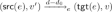 . Conversely, if \(d_0\in [0;d]\) and \(v'\in F(d_0)\) exist such that
  , then
  , and for some \(d_1\le d-d_0\),
  . Then letting \(v=v'+d-d_0\), we have \(v\in E+d\) and
  and
and  and
and  . This proves our result for this case.
 -
we finally consider the case where
 and e resets the clock. In this case,
  means that
  and
and  , which rewrites as \(0\le v\le d\) and
  . Let \(d_0=d-v\). The property above entails that \(0\le d_0\le d\), and that there exists some
 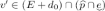 , so that \(0\le d_0\le d\), \(v'\in F(d_0)\) and
 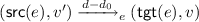 . Conversely, if those conditions hold, then for some \(0\le d_1\le d-d_0\), we have
  , and \(v=d-(d_0+d_1)\) (remember that e resets the clock). Then
  , so that
  , and finally
  .
.
 , then
  . On the other hand, for any
  , so that
  , and the transition cannot be taken from that valuation. Hence both sides of the equivalence evaluate to false, and the equivalence holds.
 , and consider the case where e does not reset the clock. Then
  means that
  . If such a v exists, then
  is non-empty: indeed, this is trivial if either
  , or
, or  , or
, or  and
and  , so that
  . Moreover,
  since
since  and
and  . Then for any
  , letting
  , so that
  . Conversely, if
  , then
  , and for some
  . Then letting
  and
and  and
and  . This proves our result for this case.
 and e resets the clock. In this case,
  means that
  and
and  , which rewrites as
  . Let
. Let  , so that
  . Conversely, if those conditions hold, then for some
  , and
, and  , so that
  , and finally
  .
.We now extend this result to sequences of transitions. The case where \(w=\bot \) is straightforward. Now assume that the result holds for some word w, and consider a word \(w\cdot e\). In case  , the result is trivial.
The case of single transitions has been handled just above. We thus consider the case of \(w\cdot e\) with  . First assume that
  , and let
  . Then
  , thus there exist \(0\le d_0\le d\) and \(v\in F'(d_0)\) s.t.
  . Since \(v\in F'(d_0)\), there must exist \(0\le d_1\le d_0\) and \(v''\in F(d_1)\) such that
  . We thus have found \(0\le d_1\le d\) such that
  .
.
Conversely, if  for some \(0\le d_1\le d\) and \(v''\in F(d_1)\), then we have
  for some \(d_0\in [d_1; d]\) and some v. We prove that
  : indeed, we have \(d_1\in [0;d_0]\), and \(v''\in F(d_1)\) such that
  , which by induction hypothesis entails
  . Thus we have \(d_0\in [0;d]\) and \(v\in F'(d_0)\), where
  , such that
  , which means
  , and concludes the proof. \(\square \)
Thanks to this semantic characterization of  , we get:
Corollary 11
For any sequence w of transitions, and any two equivalent timed sets F and \(F'\), the timed sets  and
and  are equivalent.
Finally, we extend  to linear timed markings in the expected way: given a linear timed marking M, and a sequence w of transitions, we let

Again, we have  for any
  . Then:
Lemma 12
 for all
  and all linear timed marking M.
Letting  for any subset
  of
of  , and
, and  , we immediately get:
Theorem 13
For any linear timed marking M, it holds  .
.
It follows that the closure of any marking can be represented as a linear timed marking. However, this linear timed marking is currently defined as an infinite union over all sequences of consecutive silent transitions. We make the computation more effective in the next section.
4.3 Finite Representation of the Closure
In this section, we prove that we can effectively compute a finite representation of the closure of any regular timed marking. More precisely, we show how to compute such a closure as a regular timed marking.
Finiteness. Indeed, let M be (a finite representation of) a regular timed marking: then M can be written as the finite union of atomic regular timed markings  , defined as
  and
and  for all
  . In the end, any regular timed marking M can be written as the finite union \(\bigsqcup _{i\in I} M_i\) of atomic regular timed markings. Thus we have
  , and it suffices to compute
  for atomic regular timed markings
  . We prove that those closures can be represented as regular timed markings.
We write  and
and  for the first and second components of
  . Notice that
  does not depend on E (so that we may denote it with
  in the sequel). In particular,
-
 if
if  is a sequence of consecutive transitions ending with a resetting transition;
 -
 if
if  is a sequence of consecutive non-resetting transitions.
 if
if  is a sequence of consecutive transitions ending with a resetting transition;
 if
if  is a sequence of consecutive non-resetting transitions.
Letting  , it follows that
  . for any
  and any w. Thus
  can be written as a finite union of atomic timed markings.
Regularity. To prove regularity, we first introduce some more formalism:
-
we let
 and
and  . We thus have
  ;
; -
for
 and
and  , we write
  for the interval
  ;
; -
we define a mapping
 that counts the number of occurrences of certain timing constraints at resetting transitions along a path: precisely, it is defined inductively as follows (where \(\Cup \) represents addition of an element to a multiset):
 and
and  . We thus have
  ;
; and
and  , we write
  for the interval
  ;
; that counts the number of occurrences of certain timing constraints at resetting transitions along a path: precisely, it is defined inductively as follows (where
By induction on w, we prove:
Lemma 14
Let  be a timed set with
  , and
, and  . Then

Now, we fix an atomic regular timed marking  . For any state
  of
of  , we let
  be the set of all sequences of consecutive transitions from
  to
to  in
in  . Then

Hence we need to prove that  is regular.
For any set  of sequences of consecutive transitions, and for any
  and
and  in
in  , we let
  . One easily observes that for any
  and any
  , it holds
  , so that

The following property entails that this set is a regular union of intervals:
Lemma 15
Let E be a regular union of intervals,  and
and  be two elements of
  , and
, and  be a regular language. Then
  is a regular union of intervals.
5 Experimentations
In order to evaluate the possible improvement of our approach compared to the diagnoser proposed in [26], we implemented and compared the performances of both approaches. Sources can be downloaded at http://www.lsv.fr/~jaziri/DOTA.zip.
5.1 Comparison of the Approaches
In the approach of [26], the set of possible current configurations is stored as a marking. If an action l occurs after some delay d, the diagnoser computes the set of all possible configurations reached after delay d (possibly following silent transitions), and applies from the resulting markings the set of all available transitions labelled l. This amounts to computing the functions \(\mathbf{O}_d\) and \(\mathbf{O}_l\) at each observation. There is also a timeout, which makes the diagnoser update the marking (with \(\mathbf{O}_{d}\)) regularly if no action is observed. The computation of \(\mathbf{O}_d\) is heavily used, and has to be performed very efficiently so that the diagnoser can be used at runtime.
In our approach, we use timed markings to store sets of possible configurations. Given a timed marking, when an action l is observed after some delay d, we can easily compute the set of configurations reachable after delay d, and have to apply \(\mathbf{O}_l\) and recompute the  -closure. Following [7], \(\mathbf{O}_l\) can be performed as a series of set operations on intervals. The
  -closure can be performed as a series of subtractions between an interval and regular unions of intervals (see Lemma 14). Those regular unions can be precomputed; while this may require exponential time and space to compute and store, this makes the simulation of a delay transition very efficient.
5.2 Implementation
In our experimentations, in order to only evaluate the benefits of the precomputation and of the use of \(\epsilon \)-closures in our approach compared to that of [26], we use the same data structure for both diagnosers. In particular, both diagnosers are implemented as automata over timed domains [7], where the timed domain is the set of timed markings. The only difference lies in the functions computing the action- and the delay transitions. As a consequence, both implementations benefit from the data structure we chose for representing timed intervals, which allows us to compute basic operations in linear time. Also, both structures use the same reachability graphs for either computing the sets of reachable configurations or the Parikh images.
Our implementation is written in Python3. One-clock timed automata and both diagnosers are instances of an abstract class of automata over timed markings; timed markings are implemented in a library TILib. Simulations of those automata are performed using an object called ATDRunner, which takes an automaton over timed markings and simulates its transitions according to the actions it observes on a given input channel. It may also write what it does on an output channel. A channel is basically a way of communicating with ATDRunners.
In order to diagnose a given one-clock timed automaton, stored in an object OTAutomata, we first generate a diagnoser object, either a DiagOTA or a TripakisDOTA, depending of which version we want to use. Then we launch two threads: one is an ATDRunner simulating the timed automaton, listening to some channel object Input, and writing every non-silent action it performs on some other channel object Comm. The other one is another ATDRunner simulating the diagnoser and listening to the Comm channel.
In a DiagOTA object, which corresponds to our approach, we have already precomputed the relevant timed intervals; action transitions are then made by operations over timed markings, and delay transitions are encoded by increasing a padding information on the timed markings, which is applied when performing the next action transition. In such a simulation, we can thus keep track of which states may have been reached, but also predict which states may be reached in the future and the exact time before we can reach them.
In a TripakisDOTA object, which corresponds to the approach of [26], action and delay transitions are simulated by computing all configurations reachable through that action or delay, also allowing arbitrarily many silent transitions. This does not allow for prediction.
5.3 Results
Figure 3 reports on the performances of both implementations on a small set of (randomly generated) examples. Those examples are distributed with our prototype. In Fig. 3, we give the important characteristics of each automaton (number of states and of silent transitions), the amount of precomputation time used by our approach, and the average time (over 400 random runs) used in the two approaches to simulate action- and delay transitions.

Bench for 5 examples over 400 runs with 10 to 20 actions
As could be expected, our approach outperforms the approach of [26] on delay transitions by several orders of magnitude in all cases. The performances of both approaches are comparable when simulating action transitions.
The precomputation phase of our approach is intrinsically very expensive. In our examples, it takes from less than a second to more than 13 min, and it remains to be understood which factors make this precomputation phase more or less difficult. We may also refine our implementation of the computation of Parikh images, which is heavily used in the precomputation phase.
6 Conclusion and Future Works
In this paper, we presented a novel approach to fault diagnosis for one-clock timed automata; it builds on a kind of powerset construction for automata over timed domains, using our new formalism of timed sets to represent the evolution of the set of reachable configurations of the automaton. Our prototype implementation shows the feasibility of our approach on small examples.
There remains space for improvements in many directions: first, our implementation can probably be made more efficient on the precomputation phase, and at least we need to better understand why some very small examples are so hard to handle.
A natural continuation of this work is an extension to n-clock timed automata. This is not immediate, as it requires a kind of timed zone, and an adaptation of our operator  . Another possible direction of research could target priced timed automata, with the aim of monitoring the cost of the execution in the worst case.
Notes
- 1.
In this paper, we write \(\bot \) for the empty word (or empty sequences) over any alphabet.
References
Alur, R., Dill, D.L.: A theory of timed automata. Theor. Comput. Sci. 126(2), 183–235 (1994)
Behrmann, G., et al.: Uppaal 4.0. In: Proceedings of the 3rd International Conference on Quantitative Evaluation of Systems (QEST 2006), pp. 125–126. IEEE Computer Society Press, September 2006
Bengtsson, J., Yi, W.: Timed automata: semantics, algorithms and tools. In: Desel, J., Reisig, W., Rozenberg, G. (eds.) ACPN 2003. LNCS, vol. 3098, pp. 87–124. Springer, Heidelberg (2004). https://doi.org/10.1007/978-3-540-27755-2_3
Benveniste, A., Fabre, É., Haar, S., Jard, C.: Diagnosis of asynchronous discrete event systems: a net-unfolding approach. IEEE Trans. Autom. Control. 48(5), 714–727 (2003)
Bertrand, N., Haddad, S., Lefaucheux, E.: Foundation of diagnosis and predictability in probabilistic systems. In: Raman, V., Suresh, S.P. (eds.) Proceedings of the 34th Conference on Foundations of Software Technology and Theoretical Computer Science (FSTTCS 2014). Leibniz International Proceedings in Informatics, vol. 29, pp. 417–429. Leibniz-Zentrum für Informatik, December 2014
Bouyer, P., Chevalier, F., D’Souza, D.: Fault diagnosis using timed automata. In: Sassone, V. (ed.) FoSSaCS 2005. LNCS, vol. 3441, pp. 219–233. Springer, Heidelberg (2005). https://doi.org/10.1007/978-3-540-31982-5_14
Bouyer, P., Jaziri, S., Markey, N.: On the determinization of timed systems. In: Abate, A., Geeraerts, G. (eds.) FORMATS 2017. LNCS, vol. 10419, pp. 25–41. Springer, Cham (2017). https://doi.org/10.1007/978-3-319-65765-3_2
Cassez, F.: A note on fault diagnosis algorithms. In: Proceedings of the 48th IEEE Conference on Decision and Control (CDC 2009), pp. 6941–6946. IEEE Computer Socirty Press, December 2009
Chen, Y.-L., Provan, G.: Modeling and diagnosis of timed discrete event systems - a factory automation example. In: Proceedings of the 1997 American Control Conference (ACC 1997), pp. 31–36. IEEE Computer Society Press, June 1997
Clarke, E.M., Allen Emerson, E., Sifakis, J.: Model checking: algorithmic verification and debugging. Commun. ACM 52(11), 74–84 (2009)
Clarke, E.M., Grumberg, O., Peled, D.A.: Model Checking. MIT Press, Cambridge (2000)
Clarke, E.M., Henzinger, T.A., Veith, H., Bloem, R.: Handbook of Model Checking. Springer, Cham (2018). https://doi.org/10.1007/978-3-319-10575-8
Filliâtre, J.-C.: Deductive software verification. Int. J. Softw. Tools Technol. Transf. 13(5), 397–403 (2011)
Finkel, O.: Undecidable problems about timed automata. In: Asarin, E., Bouyer, P. (eds.) FORMATS 2006. LNCS, vol. 4202, pp. 187–199. Springer, Heidelberg (2006). https://doi.org/10.1007/11867340_14
Genc, S., Lafortune, S.: Predictability of event occurrences in partially-observed discrete-event systems. Automatica 45(2), 301–311 (2009)
Henzinger, T.A., Sifakis, J.: The embedded systems design challenge. In: Misra, J., Nipkow, T., Sekerinski, E. (eds.) FM 2006. LNCS, vol. 4085, pp. 1–15. Springer, Heidelberg (2006). https://doi.org/10.1007/11813040_1
Hoare, C.A.R.: An axiomatic basis for computer programming. Commun. ACM 12(10), 576–580 (1969)
Lafortune, S., Lin, F., Hadjicostis, C.N.: On the history of diagnosability and opacity in discrete event systems. Annu. Rev. Control. 45, 257–266 (2018)
Leucker, M., Schallart, C.: A brief account of runtime verification. J. Log. Algebr. Program. 78(5), 293–303 (2009)
Lunze, J., Schröder, J.: State observation and diagnosis of discrete-event systems described by stochastic automata. Discret. Event Dyn. Syst. 11(4), 319–369 (2001)
Narasimhan, S., Biswas, G.: Model-based diagnosis of hybrid systems. IEEE Trans. Syst., Man, Cybern. Part A Syst. Hum. 37(3), 348–361 (2007)
Sampath, M., Lafortune, S., Teneketzis, D.: Active diagnosis of discrete-event systems. IEEE Trans. Autom. Control. 43(7), 908–929 (1998)
Sampath, M., Sengupta, R., Lafortune, S., Sinnamohideen, K., Teneketzis, D.: Diagnosability of discrete-event systems. IEEE Trans. Autom. Control. 40(9), 1555–1575 (1995)
Sampath, M., Sengupta, R., Lafortune, S., Sinnamohideen, K., Teneketzis, D.: Failure diagnosis using discrete-event models. IEEE Trans. Comput. 35(1), 105–124 (1996)
Tretmans, J.: Conformance testing with labelled transition systems: Implementation relations and test generation. Comput. Netw. ISDN Syst. 29(1), 49–79 (1996)
Tripakis, S.: Description and schedulability analysis of the software architecture of an automated vehicle control system. In: Sangiovanni-Vincentelli, A., Sifakis, J. (eds.) EMSOFT 2002. LNCS, vol. 2491, pp. 123–137. Springer, Heidelberg (2002). https://doi.org/10.1007/3-540-45828-X_10
Tripakis, S.: Folk theorems on the determinization and minimization of timed automata. Inf. Process. Lett. 99(6), 222–226 (2006)
Zaytoon, J., Lafortune, S.: Overview of fault diagnosis methods for discrete event systems. Annu. Rev. Control. 37(2), 308–320 (2013)
Author information
Authors and Affiliations
Corresponding author
Editor information
Editors and Affiliations
Rights and permissions
Copyright information
© 2018 Springer Nature Switzerland AG
About this paper

Cite this paper
Bouyer, P., Jaziri, S., Markey, N. (2018). Efficient Timed Diagnosis Using Automata with Timed Domains. In: Colombo, C., Leucker, M. (eds) Runtime Verification. RV 2018. Lecture Notes in Computer Science(), vol 11237. Springer, Cham. https://doi.org/10.1007/978-3-030-03769-7_12
Download citation
DOI: https://doi.org/10.1007/978-3-030-03769-7_12
Published:
Publisher Name: Springer, Cham
Print ISBN: 978-3-030-03768-0
Online ISBN: 978-3-030-03769-7
eBook Packages: Computer ScienceComputer Science (R0)