
Abstract
The advent of techniques for imaging solitary fluorescent molecules has made possible many new kinds of biological experiments. Here, we describe the application of single-molecule imaging to the problem of subunit stoichiometry in membrane proteins. A membrane protein of unknown stoichiometry, prestin, is coupled to the fluorescent enhanced green fluorescent protein (eGFP) and synthesized in the human embryonic kidney (HEK) cell line. We prepare adherent membrane fragments containing prestin-eGFP by osmotic lysis. The molecules are then exposed to continuous low-level excitation until their fluorescence reaches background levels. Their fluorescence decreases in discrete equal-amplitude steps, consistent with the photobleaching of single fluorophores. We count the number of steps required to photobleach each molecule. The molecular stoichiometry is then deduced using a binomial model.
Access provided by CONRICYT – Journals CONACYT. Download protocol PDF
Key words
1 Introduction
Observation of the fluorescence emitted by single fluorescent molecules, once difficult, is now readily performed in many laboratories. This has been made possible by improvements in detectors, primarily highly sensitive digital cameras (EM-CCD or sCMOS). One technical advance made possible by single-molecule technology is the determination of subunit stoichiometry in membrane proteins. Traditional methods of determining the stoichiometry of oligomerization, such as Western blots, often yield ambiguous results, perhaps because the protein is no longer in its native environment, the plasma membrane. An ingenious approach to this problem was described by Ulbrich & Isacoff in 2007 [1]. They expressed membrane proteins, coupled to the enhanced green fluorescence protein (eGFP), in frog oocytes. They used a high quantum efficiency electron-multiplying charge-coupled device (EM-CCD) camera and total internal reflection (TIRF) imaging to isolate single fluorescent molecules of membrane proteins. Under continuous excitation, the fluorescence of regions of interest (ROIs) enclosing putative single molecules were observed to decrease in approximately equal-amplitude steps, consistent with the photobleaching of single fluorophore molecules. By counting the number of steps to photobleach the fluorophores to background, they were able to estimate the stoichiometry of the molecule (Fig. 1). The method has since been applied by many others [2–7].

Illustration of the single-molecule subunit counting method. The figure is a hypothetical plot of the fluorescence intensity of a single tetrameric molecule, as a function of time, with each subunit covalently linked to a fluorophore, under continuous excitation sufficient to cause fluorophore photobleaching of the fluorophores. The fluorescence decreases in approximately equal amplitude steps until background levels are reached. The molecular diagrams indicate the number of active fluorophores (depicted in green) at each stage. The number of steps (in this case four) in theory yields the stoichiometry of the molecule. From [16]
We have recently applied the method to the stoichiometry of a membrane protein important in mammalian hearing, prestin [8]. The stoichiometry of prestin has been in dispute, with both dimer and tetramer configurations being advanced by Western blot analyses [9, 10], biophysical analysis [11], and an electron-density mapping of purified prestin protein [12]. We studied prestin coupled at its carboxy terminal to eGFP, incorporated in the plasma membrane of a cultured cell line. To immobilize the molecules, we prepared membrane fragments adherent to the culture dish, by osmotic shock and lysis. In this paper, we discuss our implementation of the technique and give practical suggestions for applying the method to other systems (see Notes 1 and 2 ).
2 Materials
2.1 Cell Culture, Transient Transfection, and Cell Imaging Preparation
-
1.
Culture medium: Dulbecco’s Modified Eagle Medium (DMEM) with added glucose, glutamine, and pyruvate with 10 % Fetal Bovine Serum (FBS) .
-
2.
0.25 % Trypsin-EDTA.
-
3.
Cell culture flasks: 25 mm2 surface area, with a 0.2 μm vent cap (Corning, Inc., Corning, NY).
-
4.
Glass-bottomed dishes. We use 35 mm glass-bottom dishes (MatTek Corp., Ashland, MA). Number 1.5 coverslips are essential for use with high numerical aperture (NA) objectives (see Subheading 2.4, step 2).
-
5.
Cells: Human Embryonic Kidney (HEK) cells from ATCC (Manassas, VA).
-
6.
Prestin c-terminal eGFP plasmid was obtained from the Dallos laboratory. Contact Jing Zheng (jzh215@northwestern.edu) for further information.
-
7.
Transient transfection reagents: Lipofectamine 2000 transfection reagent (Invitrogen), DMEM.
-
8.
15 mL sterile centrifuge tubes.
-
9.
Lysis and imaging hypoosmotic buffer: 4 mM PIPES, 30 mM KCl, pH 6.2, 80 mOsm.
-
10.
Cell lysis requires a 29 G hypodermic needle, blunted, on a 1 mL syringe.
2.2 Imaging and Analysis
-
1.
Microscope: The microscope should be an inverted model with a camera port, preferably 100 % switchable. We use an Olympus IX-70.
-
2.
Objective: A 100× 1.4 numerical aperture UPlanSApo objective from Olympus, and low-fluorescence non-drying immersion oil (Type HF, Cargille Laboratories, Cedar Grove, NJ).
-
3.
Excitation: A 100 W mercury lamp for wide-field UV and blue excitation, its intensity attenuated by neutral density filters (see Notes 3 and 4 ).
-
4.
Total internal reflection (TIRF) imaging may be considered as an alternative (see Note 5 ).
-
5.
Filters: High quality steep cut-off filters from Chroma (Bellows Falls, VT) or Semrock (Rochester, NY) are preferred. Our emission filter for eGFP is an ET535/30 m from Chroma.
-
6.
Detector: An Andor DU-897E back-thinned EMCCD camera with > 90 % quantum efficiency in the visible range (Andor Technology, Belfast, Northern Ireland).
-
7.
Image Acquisition: Andor Solis software for image acquisition, which is provided with the camera. To determine the single molecule image size in pixels, see Note 6 .
-
8.
Analysis: Singlmol, written in Matlab version R20008b with the Image Processing Toolbox (MathWorks, Natick, MA), which is freely available from the authors.
3 Method
3.1 Cell Preparation
-
1.
Grow HEK cells in 5 mL of DMEM plus 10 % FBS in a 25 mm2 flask in a CO2 incubator at 37 °C.
-
2.
For passage at confluence (70–90 %), liberate the cells using 2 mL per flask of 0.25 % trypsin-EDTA for 10 min in the incubator. Quench the enzyme with 3 mL of culture medium, and then spin down the cells at 40 × g for 4 min at 4 °C in a 15 mL tube. Resuspend the cells in 1 mL culture medium. Cell passage should be performed in a laminar flow hood. Start new cells from stocks once the passage number reaches 30.
-
3.
To plate passaged cells for experimentation, incubate glass-bottom dishes containing culture medium for 20 min in the incubator. Add the resuspended cells to the dishes. Adjust the volume of cells so that the dishes reach 70 % confluence after 3 days. Cell plating should be performed in a laminar flow hood.
-
4.
Transfection: Transfect cells with 15 μg of plasmid per dish using Lipofectamine 2000 the day after plating. Follow the manufacturer’s instructions for preparation of transfection medium. Transfection should be performed in a laminar flow hood.
-
5.
Cell Lysis (Fig. 2): Remove a dish of cells from the incubator, then remove the culture medium by aspiration and replace it with cold lysis medium. Incubate on ice for 30 min. Remove adherent cells using a stream of cold lysis buffer forced through a 29 G needle. Replace the lysis medium with fresh lysis medium to remove cell fragments. Allow the dish to come to room temperature before imaging in lysis medium, or any medium without pH-sensitive dyes such as Phenol Red.
Fig. 2 
The osmotic shock and lysis method of preparing membrane fragments. Starting at left, the cell containing fluorophore-conjugated molecules in its membrane is exposed to a hypoosmotic solution causing it to swell and its membrane to weaken. The cell is exposed to a stream of buffer, which lyses the cell and removes its contents, leaving behind basolateral membrane fragments containing immobilized fluorescent molecules (right)

3.2 Imaging Procedure
-
1.
Experiment in a darkened room to minimize collection of stray light. Cover the microscope with photographic darkroom cloth.
-
2.
Establish the focal plane using the camera image, then translate the specimen in the x- or y-direction a small amount, but greater than one image field, and only then start data acquisition. Similarly, stop down the excitation field so that it is no more than the camera’s field of view. The focal plane must be established exactly for maximum fluorophore brightness, but it is equally important to minimize photobleaching during establishment of the focal plane, since exposure to even the attenuated UV excitation that we use results in some photobleaching, which subtracts potentially detectable steps.
-
3.
Acquire images stacks under UV excitation at 5 frames/s until all single molecules are photobleached (usually 500–1000 frames). Use electron-multiplying gain s of 100–200 and cool the electronics to −70 °C to reduce noise. Save files as 12-bit TIFs.
3.3 Analysis Procedure
-
1.
Import image stacks into MatLab for analysis using the Singlmol script. The user interface of the code is shown in Fig. 3. The program subjects the images to two passes of a 3 × 3 Gaussian spatial filter to reduce noise before display and analysis. The interface enables background subtraction, thresholding and gain adjustment of the images and permits them to be viewed in sequence. Sequential viewing assists in separating transient high-value points from the persistent fluorescence of single molecules.
Fig. 3 
The user interface of program Singlmol. The left window shows a single frame, with sliders controlling display maximum and minimum on top and the sequence counter at right. The images show typical large clumps of fluorescent molecules (labeled “Macromolecular Clusters”) and some putative single molecules, one of which is indicated by the rectangular region of interest (labeled “ROI”). An enlarged view of the ROI is shown in the window at right (labeled “ROI Window”). The time plot below right shows the average fluorescence in the ROI over the acquisition period, with the background subtracted. Cursors were used to establish the steps. Labels on the plot indicated apparent single steps and a double step
-
2.
Perform background subtraction by first selecting an ROI close to but not encompassing the single molecule of interest (click on BacSelect). Some background fluorescence is always observed, although inconsistent across the field of view, and it decays approximately exponentially over the imaging period. The program determines and plots the average background fluorescence in the ROI as a function time. Accept the function by clicking on the Accept button on the plot. To use background subtraction, click on BacSubOn.
-
3.
Click on the ROI button to select an ROI containing a putative single molecule for analysis, via a cursor. The program shows an enlarged image of the 5 × 5 displayed ROI in a separate window for inspection. Adjust the cursor position if the single molecule image is not centered over time (individual images may not appear centered). The average fluorescence in the ROI as a function of time is then calculated and the background values subtracted. The program then subjects the background-subtracted fluorescence values to a three-point median filter and plots the result in a separate window, with upper and lower plot bounds that can be manipulated for ease of viewing.
-
4.
The corner points of the square ROI are farther from the centroid of the image than the Airy disk radius, and thus contribute little information. In calculating the average ROI fluorescence, the program employs a mask that zeros the corner points of the ROI thereby reducing the noise without sacrificing the fluorescence in the Airy disk image. The mask is:
\( \left[\begin{array}{c}0\kern0.28em 0\kern0.28em 1\kern0.28em 0\kern0.28em 0\\ {}0\kern0.28em 1\kern0.28em 1\kern0.28em 1\kern0.28em 0\\ {}1\kern0.28em 1\kern0.28em 1\kern0.28em 1\kern0.28em 1\\ {}0\kern0.28em 1\kern0.28em 1\kern0.28em 1\kern0.28em 0\\ {}0\kern0.28em 0\kern0.28em 1\kern0.28em 0\kern0.28em 0\end{array}\right] \)
-
5.
Click on the Analyze button to measure the step sizes. Use cursors to delineate time ranges corresponding to the beginning and end of fluorescence levels corresponding to two discrete states. The program calculates the average fluorescence in those two states and the difference between them, which is the step size. Repeat the operation until all steps have been measured for that molecule. Store the step sizes in a file by clicking on the Save button. To start over, click on the Clear button.
-
6.
Import the saved data for that image sequence into Excel. Calculate the average step size for the entire image sequence. Inspect the step sizes for each molecule and manually enter the step count in a separate column. Use the average step size to arbitrate any steps not clearly unitary (see Notes 7 and 8 ). Sort the step counts into a histogram using the Histogram function of Excel. Usually, at least 100 molecules must be studied to obtain a histogram that can be analyzed. An example of the results is shown in Fig. 4
Fig. 4 
Representative example of the analysis of single molecules of prestin -eGFP. Histograms of step amplitudes (a) and step counts (b) in a single experiment, for 2315 molecules. The binomial fit parameters are given in the figure. From [16]


3.4 Fitting the Binomial Distribution
-
1.
Rationale for the Binomial Fit. If a molecule is a tetramer , then the step count ought in theory to be four for every molecule. We observe instead that some molecules exhibit four steps, but more exhibit three, some two, and a few even exhibit a single step. Our model, discussed in greater detail in Note 9 , is that some eGFP fluorophores do not fluoresce. Thus, a single molecule composed of randomly selected prestin-eGFP molecules with fluorescing and non-fluorescing eGFPs will have an unknown number of fluorescing eGFPs. The distribution of step counts , representing the number of fluorescing eGFPs, will be described by a binomial distribution, where n represents the molecular stoichiometry and p represents the average fraction of functioning fluorophores in a given experiment (see also Note 10 ).
-
2.
Distinguishing Between Possible Stoichiometries. It is not possible to use a goodness-of-fit comparison between different putative stoichiometries because the number of points fitted, and therefore the number of degrees of freedom, is different in each case. We have therefore used two methods to establish stoichiometry.
-
One is to use a molecule of known stoichiometry for comparison [8]. If the same fluorophore is used, and if the p values are similar, then the stoichiometries are likely to be the same.
-
Another approach is to establish a baseline value of p, p 0 , for the fluorophore using a molecule of known stoichiometry [13]. For molecules of unknown stoichiometry, first calculate the mean of the distribution μ. Then n is calculated as μ/p 0, rounding to the nearest integer.
-
4 Notes
-
1.
In principle, this method will work with other fluorescent proteins or organic fluorophores. However, antibody-conjugated fluorophores are inappropriate because multiple fluorophores are attached to each secondary antibody , and an unknown number of secondary antibodies will have bound to the primary antibody. With any fluorophore, the experimenter must balance the need to minimize bleaching with the need for sufficient brightness for single molecules to be detectable.
-
2.
The method can be readily applied to determining hetero-oligomeric stoichiometries in membrane oligomers, by combining labeled and unlabeled component monomers. It can also be applied to cytoplasmic proteins if the proteins can be isolated and immobilized.
-
3.
The excitation should be properly centered at 100× and should be as even as possible. This may be assisted by a slight defocus after normal adjustment. Note that mercury bulbs rapidly lose brightness and stability toward the end of their lives. It is wise to start a new series of experiments with a new bulb. Allow 24 h or so of operation to stabilize a new bulb.
-
4.
The excitation intensity at the specimen is severely attenuated by neutral density filters. This is to prolong the time required to bleach the molecules. We use a stack of 25 mm neutral density filters from ThorLabs Inc. (Newton, NJ) mounted in a custom-built holder.
-
5.
Observation of fluorescent proteins in membranes may seem like a natural application of TIRF imaging. Indeed, the reduced excitation levels afforded by TIRF may help to reduce the rate of bleaching. However, the background-rejection advantages of TIRF imaging are less apparent in our isolated membrane fragment preparation, since most of the background-contributing cellular contents have been removed. In addition, TIRF systems suffer from fringing due to internal reflections of polarized light, and the image field is usually unevenly illuminated. In our hands, this contributed to a greater scatter in the estimates of single step size, which led us to return to wide-field illumination.
-
6.
A point source of light, such as a fluorophore, when processed by an imaging device such as a microscope, is observed in the form of a spatial function referred to as an Airy function (Fig. 5). The radius at the first minimum, r 0, (the Airy disk radius, which encompasses approximately 84 % of the light in the image, is given by
Fig. 5 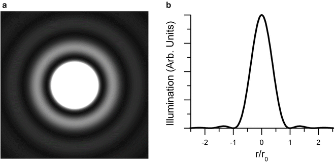
The image of a point fluorescence source in a microscope. (a) Simulation of the image of a single source, in the form of an Airy disk . (b) Plot of illumination of the Airy disk as a function of normalized radial distance from the centroid, normalized to r 0. From [16]
$$ {r}_0=0.61\lambda /na $$where λ is the wavelength of the light and na is the numerical aperture of the microscope objective. For our experiments, using eGFP, the objective na was 1.4 and we assumed λ = 520 nm. This led to a calculated Airy disk diameter of 450 nm. We used a stage micrometer to determine the pixel size of our camera image, and thereby determined that a single molecule would comfortably fit in a 5 × 5 pixel ROI.
-
7.
There is an upper limit to the stoichiometries that this method can assess because the shot noise (noise associated with the random arrival of photons) increases as the square root of the number of subunits, while the step size remains constant. In our hands this limit is seven.
-
8.
We have experimented with several methods of automating the determination of step counts, including Hidden Markov Modeling [14] and the Chung–Kennedy algorithm [15]. However, each method requires some empirical determination of parameters. In-side-by-side comparisons, we found no difference in the results.
-
9.
As we and others have reported [1, 8], the number of steps is variable from molecule to molecule, and the mean step count is non-integer. One explanation is that a fraction of fluorescent proteins fold correctly but do not fluoresce. Thus the experiment resembles a binomial sampling procedure, in which a small sample of n items is removed without replacement from a larger population, some of which are defective. If the probability that the individual item is defective is q, the probability that it is not defective is p, which is 1 − q. Our observations can then be understood if q is the probability that the fluorophore is defective. The distribution of step counts for N observations of single molecules is then given by:
$$ A(x)=N\frac{n!}{x!\left(n-x\right)!}{p}^x{\left(1-p\right)}^{n-x},\kern1.28em x=0,\kern0.28em 1,\kern0.28em 2,\dots, n $$where A(x) is the number of single molecules that bleached in x steps (and x is an integer), N is the number of single molecules observed, n is the presumed stoichiometry (also integer), and p is the fraction of fluorophores that are functional (0 < p < 1). The mean of the binomial sampling distribution μ is equal to np.
-
10.
As is clear from Fig. 4, with prestin we occasionally observed step counts greater than four. We assume that these ROIs contained two or more prestin molecules.

References
Ulbrich MH, Isacoff EY (2007) Subunit counting in membrane-bound proteins. Nat Methods 4:319–321
Bartoi T, Augustinowski K, Polleichtner G et al (2014) Acid-sensing ion channel (ASIC) 1a/2a heteromers have a flexible 2:1/1:2 stoichiometry. Proc Natl Acad Sci U S A 111:8281–8286
Das SK, Darshi M, Cheley S et al (2007) Membrane protein stoichiometry determined from the step-wise photobleaching of dye-labelled subunits. Chembiochem 8:994–999
Durisic N, Godin AG, Wever CM et al (2012) Stoichiometry of the human glycine receptor revealed by direct subunit counting. J Neurosci 32:12915–12920
Hastie P, Ulbrich MH, Wang HL et al (2013) AMPA receptor/TARP stoichiometry visualized by single-molecule subunit counting. Proc Natl Acad Sci U S A 110:5163–5168
Ji W, Xu P, Li Z et al (2008) Functional stoichiometry of the unitary calcium-release-activated calcium channel. Proc Natl Acad Sci U S A 105:13668–13673
Lioudyno MI, Kozak JA, Penna A et al (2008) Orai1 and STIM1 move to the immunological synapse and are up-regulated during T cell activation. Proc Natl Acad Sci U S A 105:2011–2016
Hallworth R, Nichols MG (2012) Prestin in HEK cells is an obligate tetramer. J Neurophysiol 107:5–11
Detro-Dassen S, Schanzler M, Lauks H et al (2008) Conserved dimeric subunit stoichiometry of SLC26 multifunctional anion exchangers. J Biol Chem 283:4177–4188
Zheng J, Du GG, Anderson CT et al (2006) Analysis of the oligomeric structure of the motor protein prestin. J Biol Chem 281:19916–19924
Wang X, Yang S, Jia S et al (2010) Prestin forms oligomer with four mechanically independent subunits. Brain Res 1333:28–35
Mio K, Kubo Y, Ogura T et al (2008) The motor protein prestin is a bullet-shaped molecule with inner cavities. J Biol Chem 283:1137–1145
Hallworth R, Stark K, Zholudeva L et al (2013) The conserved tetrameric subunit stoichiometry of Slc26 proteins. Microsc Microanal 19:799–807
McKinney SA, Joo C, Ha T (2006) Analysis of single-molecule FRET trajectories using hidden Markov modeling. Biophys J 91:1941–1951
Chung SH, Kennedy RA (1991) Forward-backward non-linear filtering technique for extracting small biological signals from noise. J Neurosci Methods 40:71–86
Hallworth R, Nichols MG (2012) The single molecule imaging approach to membrane protein stoichiometry. Microsc Microanal 18:771–780
Acknowledgments
This work was supported by the State of Nebraska LB 692 administered by Creighton University and N.S.F.-Nebraska E.P.S.Co.R. EPS-0701892 to RH, and National Institutes of Health GM085776 to MGN and RH. Research was conducted in a facility constructed with support from Research Facilities Improvement Program C06 RR17417-01 from the late, lamented N.C.R.R. of N.I.H. We thank Max Ulrich and Ehud Isacoff for initial encouragement and advice, Peter Dallos for the prestin-eGFP plasmid constructs, and David Z.Z. He, Heather Jensen-Smith and John Billheimer for comments on the manuscript. We also thank Fang Xiang & Chris Wichman for statistical advice.
Author information
Authors and Affiliations
Editor information
Editors and Affiliations
Rights and permissions
Copyright information
© 2016 Springer Science+Business Media New York
About this protocol
Cite this protocol
Nichols, M.G., Hallworth, R. (2016). The Single-Molecule Approach to Membrane Protein Stoichiometry. In: Sokolowski, B. (eds) Auditory and Vestibular Research. Methods in Molecular Biology, vol 1427. Humana Press, New York, NY. https://doi.org/10.1007/978-1-4939-3615-1_11
Download citation
DOI: https://doi.org/10.1007/978-1-4939-3615-1_11
Published:
Publisher Name: Humana Press, New York, NY
Print ISBN: 978-1-4939-3613-7
Online ISBN: 978-1-4939-3615-1
eBook Packages: Springer Protocols