Fluorescence Recovery After Photo-Bleaching (FRAP) and Fluorescence Loss in Photo-Bleaching (FLIP) Experiments to Study Protein Dynamics During Budding Yeast Cell Division

Abstract

The easiness of tagging any protein of interest with a fluorescent marker together with the advance of fluorescence microscopy techniques enable researchers to study in great detail the dynamic behavior of proteins both in time and space in living cells. Two commonly used techniques are FRAP (Fluorescent Recovery After Photo-bleaching) and FLIP (Fluorescence Loss In Photo-bleaching). Upon single bleaching (FRAP) or constant bleaching (FLIP) of the fluorescent signal in a specific area of the cell, the intensity of the fluorophore is monitored over time in the bleached area and in surrounding regions; information is then derived about the diffusion speed of the tagged molecule, the amount of mobile versus immobile molecules as well as the kinetics with which they exchange between different parts of the cell. Thereby, FRAP and FLIP are very informative about the kinetics with which the different organelles of the cell separate into mother- and daughter-specific compartments during cell division. Here, we describe protocols for both FRAP and FLIP and explain how they can be used to study protein dynamics during cell division in the budding yeast Saccharomyces cerevisiae. These techniques are easily adaptable to other model organisms.

1 Introduction

During vegetative growth, the budding yeast S. cerevisiae divides asymmetrically into a bigger mother cell and a smaller daughter cell, the bud. This process starts with the bud appearing on the surface of the mother in S-phase , continues through mitosis when the duplicated chromosomes segregate into the two cells and ends with cytokinesis, which gives rise to two separated cells. All these steps rely on the function of many proteins whose behavior is often highly dynamic both in space and time. A remarkable example are septins, small GTPase proteins showing a highly dynamic behavior during cell division: upon bud emergence, at the beginning of S-phase, septins assemble in a fluid, ring-like structure at the base of the bud. At this stage, the septins diffuse easily within the ring and exchange with the cytoplasmic pool. Throughout the following phase of bud growth, the septin ring localizes to the mother–bud neck (the constriction between the mother and the future daughter cell) and forms a frozen, hourglass-like collar, within which septins are essentially immobile. Finally, during cytokinesis, when the septin ring splits and the mother and daughter cells separate from each other, septins become transiently dynamic again, before freezing in two rings, one on each side of the cleavage site [1–3].

During bud growth, the membrane proteins of the endoplasmic reticulum (ER), which diffuse relatively rapidly in the plane of the membrane, soon stop exchanging between the mother and the daughter ER [4–6]. Similarly, the outer nuclear membrane proteins (such as the reporter NSG1) and the nuclear pores (as visualized by tagging core nuclear pore components such as Nup49 and Nup170) are also restricted in their ability to freely diffuse from the mother to the daughter part of the dividing nucleus [7, 8].

Over the years, fluorescence microscopy techniques (i.e. FLIP and FRAP ) have been developed to look at these spatio-temporal dynamic processes and this has allowed scientists to obtain insights into a wealth of cellular processes. Both FLIP and FRAP rely on tagging a specific protein of interest with a genetically encoded fluorescent tag (e.g. GFP , Green Fluorescent Protein) to visualize the protein of interest in living cells. In a typical FRAP experiment, a laser is pointed to a specific region of the cell to bleach the fluorescent signal of the protein in that area; the bleaching is performed only once and subsequently the recovery of the signal in the bleached area as well as its intensity profile in the surrounding areas are monitored over time. The fluorophore intensity profile in the bleached area is then usually fit to a mathematical model (e.g. an exponential recovery, see Subheading 3 for details): this enables to obtain both kinetic information (e.g. diffusion speed of the molecule of interest) as well as non-kinetic information (e.g. the amount of mobile versus immobile molecules). On the other hand, in a typical FLIP experiment, bleaching is repeated constantly during the entire time window of the experiment and the decay of the signal from the surrounding areas is monitored over time. The decay profiles from different regions of the cell are subsequently fit to a model (e.g. one- or two-phase exponential decay, see Subheading 3 for details): on one side, this enables obtaining kinetic information such as the diffusion speed of the molecule of interest; but, most importantly, the intensity profiles obtained in FLIP experiments can be used also to extract valuable information about the structural organization of the compartment where the tagged molecule is found: for example, a speed of decay which, upon constant bleaching, stays the same all over the entire compartment would indicate that the compartment is a continuous structure; on the other hand, a difference in speed of decay between different areas of the compartment would suggest the presence of different domains that are not freely communicating with each other.

Here, we present detailed protocols for both FRAP and FLIP experiments which enable the analysis of such dynamic phenomena during cell division in Saccharomyces cerevisiae . For practical reasons, we divided the “Materials” and the “Methods” sections in different subheadings. The subheadings 2.1, 2.2 and 2.3 refer to the “Materials” section; the subheadings 3.1, 3.2 and 3.3 refer to the section “Methods”. More specifically:

• Subheading 2.1 describes the features of the yeast strains we used in this work as well as how they are constructed.

• Subheading 2.2 lists the composition of all the required media and reagents.

• Subheading 2.3 lists the needed microscopy equipment.

• Subheading 3.1 explains the sample preparation procedures.

• Subheading 3.2 explains the imaging settings. This section is divided into four subsections, respectively: “laser settings” to adjust the laser power; “time series settings” where the time resolution of the experiment is set; “bleaching settings” where the intensity and frequency of the bleaching is set, this subsection is where the main difference between FLIP and FRAP experiments is found; the last subsection, “start experiment,” explains how to start the imaging. Note that most of the settings described in Subheading 3.2 are the same between FLIP and FRAP experiments and, unless otherwise stated, they apply to both techniques.

• Subheading 3.3 explains in details the data analysis procedures. We decided to divide this section into two subsections: one relative to FRAP experiments and the other relative to FLIP experiments. Both FRAP and FLIP subsections explain first how to perform the intensity measurements and then how to fit a mathematical model to the experimental data and how to retrieve biological information out of the model. It is important to stress out that in the data analysis section we will refer to specific examples shown in the different figures. We believe that by understanding these examples and adapting what we explain to his/her specific needs, the experimenter will be easily able to perform FRAP and FLIP in his/her condition of interest.

2 Materials

Prepare all materials in deionized water. Unless otherwise specified, only the growth media are sterilized. There is no need of sterile water. Unless otherwise stated, store all reagents at room temperature. The following reagents-media are the same for FLIP and FRAP experiments (see Note 1 ).

2.1 Yeast Strains

• 1. A list of strains used in this work is shown in Table 1. All strains are isogenic to either W303 or S288C (Table 1) and were constructed according to standard genetic techniques [9].

  Table 1 S. Cerevisiae strains used in this work

2.2 Media

All the following indicated amounts are for 1 l of total volume.

• 1. YPD solid-rich media (plates): Yeast Extract 10 g, bactopeptone 20 g, 2 % glucose, 20 mg adenine, Agar Agar SERVA high gel-strength 20 g.

• 2. Selective liquid –TRP synthetic media: 2.5 g Ammonium sulfate, 850 mg Yeast Nitrogen Base without both amino acids and ammonium sulfate, 2 % glucose, 10 mg adenine, 74 mg drop out –TRP (tryptophan) mix containing all amino acids but tryptophan.

• 3. Selective solid –TRP synthetic media: 2.5 g Ammonium sulfate, 850 mg Yeast Nitrogen Base without both amino acids and ammonium sulfate, 2 % glucose, 10 mg adenine, Agar Agar SERVA high gel-strength 20 g, 74 mg drop out –TRP (tryptophan) mix containing all amino acids but tryptophan.

2.3 Microscopy Equipment

• 1. 25 mm diameter round glass coverslips (Thermo Scientific) (Fig. 1).

  Fig. 1

  

  Attofluor cell chamber used for FLIP and FRAP microscopy experiments. The cell suspension is placed as indicated between the round glass coverslip and the synthetic medium agar pad. The cell chamber is closed by screwing together its top and bottom sections. Another round glass coverslip (not depicted) is dropped on top of the cell chamber. See text for details about the sample preparation

• 2. Metallic circular Attofluor Cell chamber for microscopy (to mount the coverslip and the agar pad, see Subheading 3.1 and see Note 3 , Fig. 1 for details).

• 3. Cylindrical metallic support to cut small circular agar pads (see Subheading 3.1 for details) (see Note 3 ).

• 4. Confocal microscope (e.g. Carl Zeiss NLO 780) with a Plan-Apochromat 63X/1.4 NA (numerical aperture) oil immersion objective, an argon laser (488 nm line or other line of interest, depending on the used fluorophore), a photomultiplier detector system (PMT), an appropriate filter (e.g. 505 nm long-pass filter for GFP ) to select for the desired fluorophore and a temperature-controlled imaging chamber.

3 Methods

Unless otherwise indicated, perform all the described steps at room temperature.

Note that, unless otherwise stated, the following steps apply to both FLIP and FRAP experiments.

3.1 Sample Preparation

• 1. Before the imaging, prepare a culture by streaking some yeast cells on YPD solid media (see Note 2 ). If willing to analyze mitotic cells, let the cells grow until exponential phase.

• 2. Unscrew the Attofluor cell chamber and mount into it a circular 25 mm glass coverslip (Fig. 1 and see Note 3 ). Do not touch the coverslip on its surface.

• 3. Screw the metallic cell chamber back.

• 4. Drop in the middle of the mounted coverslip not more than 10 μl of –TRP liquid media (see Note 4 ).

• 5. With a pipette, take a few cells previously plated on YPD solid media (step 1 above) and resuspend them in the 10 μl of –TRP previously dropped on the coverslip.

• 6. With any available tool, cut a circular agar pad of –TRP solid media and put it on top of the cell suspension. Then put another 25 mm round glass coverslip on top of the agar pad.

• 7. The sample is now ready to be imaged: if desired, bring the microscope chamber up to 30 °C, then put abundant immersion oil on top of the 63X/1.4 NA microscope objective and fix the sample above the objective.

3.2 Imaging

3.2.1 Laser Settings

• 1. Launch the imaging software and set the argon laser excitation line wavelength to the desired value (for the FRAP –FLIP experiments shown in this work the wavelength was set to 488 nm, see Note 5 ).

• 2. Set the laser output (in the FRAP and FLIP experiments shown here we used 40–45 %; 2–3 % of this output was then used for imaging, see Note 6 ).

3.2.2 Time Series Settings

• 1. Set the desired time interval. In FRAP experiments, we acquired one frame every 10 s; this interval was 3–6 s for FLIP experiments (see Notes 7 and 9 ).

• 2. Set the number of cycles. This defines the entire duration of the movie. In FRAP –FLIP experiments shown in this work we set 40–60 cycles (see Note 8 ).

3.2.3 Bleaching Settings

• 1. Set the laser intensity to be used for bleaching. For the FRAP –FLIP experiments shown here, we used 80–100 % of the laser output set in the laser settings (see Subheading 3.2.1 above). See Note 9 for further details.

• 2. Set the number of iterations: this number defines how many times the laser will go through the selected region in order to bleach the signal. In this work, this number was set on 80–110 (see Note 9 ).

• 3. Set when the bleaching must start and how often it has to be performed. For FRAP experiments, we performed only one single bleaching at the beginning of the movie. For FLIP experiments, a bleaching-acquisition cycle was performed for each time frame (see Note 10 ).

3.2.4 Start Experiment

• 1. Once all the imaging settings are defined, chose a good field where a cell of interest (see Note 11 ) and at least two control cells are present (see Note 16 ).

• 2. If necessary, zoom in to reduce the field of view to a window including only the cells of interest.

• 3. Using a drawing tool, draw on the cell of interest a small region where the bleaching will be performed (Fig. 2a, b; see Note 9 ).

  Fig. 2

  

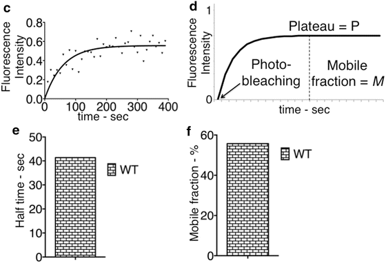
  Wild-type mitotic (a) and G1/S (b) cells expressing the septin ring component CDC12 tagged with GFP . T ₀ and T ₁, respectively, refer to the first and the second time frame of the movie. The single photo-bleaching was performed in the region “A” and the fluorescence intensity was measured in the red-labeled rectangular-like regions (see text for details). (c) Graph showing the fluorescence intensity recovery in the region “A” from a wild-type cell where the photo-bleaching was performed on half of the septin ring as in Fig. 2b. The fluorescence intensity is plotted on the Y axis over time (X axis). The data points were fit to a one-phase association function (exemplification in 2D). (d) Graph showing the one-phase association equation and its relative graph (see text for details). The fluorescence intensity recovery is plotted against time and the plateau (P), the fraction of mobile molecules (M = P) and the time of photo-bleaching (second time frame, T ₁) are indicated. (e, f) Half time (measured as Ln2/K) and mobile fraction (in percentage) measured from the one-phase association model fit to the data in C (see text for details)

• 4. For each cell and for each time point, acquire both the fluorescent (e.g. GFP ) and the transmission images. The transmission channel can be helpful in following the cell cycle stage.

• 5. Start the experiment and repeat the same procedure to acquire the desired number of cells (see Note 12 ).

• 6. Collect at least 30–40 data sets for each strain in three different experiments preferably on different days. A fraction of data sets may be unusable because of the focal plane shifted or the cell moved (see Notes 12 and 13 ).

3.3 Data Analysis

3.3.1 FRAP

• 1. Discard cells where the focal plane shifts and/or the cells move (see Note 13 ). Open the raw file with the software Image-J (FIJI can also be used) and split the two channels (transmission and GFP ) apart (for Image-J follow the path: menu “Image” > “color” > “split channels”) (see Note 14 ).

• 2. In the Image-J menu “Analyze” > “set measurements,” click on either “integrated density” or “mean gray value”; in the FRAP experiments shown here we always measured the mean gray value and we kept the selection area constant (see Note 15 ).

• 3. Using the rectangular selection tool, draw several rectangular regions around the areas where you want to measure the fluorescence intensity (examples in Fig. 2a, b). For each movie (with the cell of interest and at least two control cells) measure as follows:

  • A = Bleaching region (half of the septin ring). Here we measure the recovery after the bleaching event.

  • B = Non-bleached region: here we monitor what happens to the non-bleached half of the ring.

  • BG-CELL = Background signal for the cell of interest (see Note 17 ).

  • C1 and C2 = Signal intensity for two control cells (see Note 16 ).

  • BG-C1 and BG-C2 = Background signal of the two control cells.

• 4. For each of the time frame of the movie and for each single cell of interest, compute as follows:

  • A–BG-CELL (to subtract the background signal from the recovery measured in the bleached region).

  • B–BG-CELL (to subtract the background signal from the recovery measured in the non-bleached region).

  • The difference A–BG-CELL at t = 0 (first time frame) will be (A–BG-CELL) _t0. The same applies to the other time frames and to the difference B–BG-CELL.

  • C1–BG-C1 and C2–BG-C2 to subtract the background signal from the intensity profile measured for the two control cells.

  • The difference C1–BG-C1 at t = 0 (first time frame) will be (C1–BG-C1) _t0. The same applies to the second control cell and to the other time frames.

  • Decay of the control cell 1: (C1–BG-C1) _t0 × 100⁄(C1–BG-C1) _t0. For the second time frame it will be: (C1–BG-C1) _t1 × 100⁄(C1–BG-C1) _t0. And so on for the other time frames. The same applies to the second control cell.

  • Decay of the control cells: This is computed by simply averaging for each single time frame of the movie the decays of the two single control cells. For example, this will give us (Average Decay Control) _t0 for the first time frame. Repeat the same for the other time frames.

  • Recovery of the bleached region: for the first time frame this will be: ((A–BG-CELL) _t0 × 100⁄(A–BG-CELL) _t0)⁄(Average Decay Control) _t0. For the second time frame: ((A–BG-CELL) _t1 × 100⁄(A–BG-CELL) _t0)⁄(Average Decay Control) _t1. Repeat this for the other time frames to get the complete profile of fluorescence recovery.

  • Recovery of the non-bleached region: for the first time frame this will be: ((B–BG-CELL) _t0 × 100⁄(B–BG-CELL) _t0)⁄(Average Decay Control) _t0. For the second time frame you will compute: ((B–BG-CELL) _t1 × 100⁄(B–BG-CELL) _t0)⁄(Average Decay Control) _t1. Repeat this for the other time frames to get the complete profile of fluorescence recovery.

• 5. Plot singularly all the recovery profiles measured for the bleached and the non-bleached region for each single cell. In Fig. 2c, we show an example of the recovery measured in the bleached area after bleaching half of the septin ring as in Fig. 2b.

• 6. Once you obtain the recovery profiles, a good way to extract biological information from them is to fit these experimental data with a model. Deciding which model to use is a key step for the analysis (see Note 18 ). For the FRAP experiments shown here, we used a one phase association model described by the equation: $Y={Y}_0+\left(P-{Y}_0\right)\times \left(1- \exp \left(-KX\right)\right)$ where Y ₀ is the Y value at t = 0 (first time frame), P is the plateau value and K is the rate constant, expressed in reciprocal of the X axis time unit (see Fig. 2d for an exemplification of a one-phase association).

• 7. Once the model is chosen, define which constrain to apply to the key parameters (e.g. Y ₀, P and K, see Note 19 ).

• 8. Fit the data for each single cell and go through the results to verify the goodness of the fit (see Note 20 ).

• 9. For each cell, take the half time and average this among all the cells to get a single half time. Compute the error on this average (e.g. as standard deviation) (Fig. 2e, see Note 21 ).

• 10. For each cell, take the plateau and average this among all the cells to get a single plateau value. Compute the error on this average (e.g. as standard deviation) (Fig. 2f, see Note 22 ).

• 11. Compare the different conditions among each other. When comparing the mean, a Student’s t-test can be used to determine the statistical difference among different conditions (see Notes 12 , 23 and 24 ).

3.3.2 FLIP

• 1. In order to extract the relevant fluorescence information from the acquired image, images should be analyzed by eye to discard any images where parts of the organelle/cells of interest are out of focus (see Note 13 ).

• 2. Open the raw file with the software Image-J and split the two channels (transmission and GFP ) apart (for Image-J follow the path: menu “Image” > “color” > “split channels”) (see Note 14 ).

• 3. Using the ImageJ polygonal selection tool, select and save six regions of interest. These regions should include the organelles/cells of interest during the entire course of the acquisition process (e.g. the nucleus growing in the bud during nuclear division, Fig. 3a, b) and should include the following:

  Fig. 3

  

  (a) Wild-type anaphase cells expressing the nuclear pore component Nup49 tagged with GFP . T ₀ and T _final indicate, respectively, the first and the last time frame of the movie. The fluorescence intensity was measured in the red-labeled polygonal regions (see text for details). The red-labeled polygonal regions include the entire area over which the nuclei move over the course of the experiment. Note that “B” in the left panel (T ₀) is larger than the region of the actual daughter nucleus, but the daughter nucleus grows to the size of Bn at T _final. (b) Wild-type metaphase cells expressing the ER integral membrane protein Sec61 tagged with GFP. T ₀ and T _final indicate the first and the last frame of the movie, respectively. The yellow-labeled region indicates the area where the photo-bleaching is performed. The fluorescence intensity was measured in the indicated red-labeled regions (see text for details)

  • Compartment 1 (mother compartment; M).

  • Compartment 2 (daughter–bud compartment; B).

  • Control cell 1 (c1).

  • Control cell 2 (c2).

  • Control cell 3 (c3).

  • Background (BG).

    In this case the organelle of interest is the dividing yeast nucleus/ER, which is further divided into the mother and daughter “halves.”

• 4. Under “Analyze” > “Set Measurements”, click on either “Mean grey value” or “Integrated Density” (see Note 15 ).

• 5. For each movie (with the cell of interest and at least two control cells) and for each time frame, measure the intensity in the selected areas to obtain raw intensities for the mother and daughter nuclei/ER as well as for the control cells.

• 6. Normalize the data by the background fluorescence. To do this, simply subtract the background fluorescence from the raw mother and daughter nuclei/ER intensities (M and D), as well as the three control cells (C1, C2, and C3) obtained in 5. Note that this must be done individually for every time point; for example at time t for the M compartment you have:

  • M ^t = raw M ^t − BGt.

• 7. Photo-bleaching simply due to the acquisition process must also be corrected for. To control for this, the mother or daughter nuclear compartments (M and D) are divided by the average of the corrected control cells (after BG subtraction):

  • Corrected M ^t = M ^t /<C ^t > where < C ^t > = (C1^t + C2^t + C3^t )/3.

• 8. At this point, we have for a single cell and for all the compartments of interest (e.g. M and D) corrected fluorescence intensities profiles. Being interested in the fluorescence loss relative to the initial fluorescence measurement (M ^t0 and D ^t0), normalize each time frame of these profiles by its corresponding initial fluorescence measurement:

  • Final M ^t(i) = corrected M ^t(i) /corrected M ^t0.

• 9. Repeat this for all the time points and for all the compartments of interests. This will yield the final fluorescence decay profiles.

• 10. In order to extract biological information from the decay profiles, we must first fit the data according to an appropriate model (see Note 18 ).

• 11. Once the model is defined, define which constrain to apply to the key parameters (e.g. Y ₀, P, and K). For FLIP experiments, we constrained Y ₀ to 100 and the plateau > 0 (see Note 19 ).

• 12. Take the FLIP decays for the M and the D compartments (each containing all the analyzed cells) and fit these data as two ensemble measurements (mother and bud) with one single fit (see Note 20 ). In the experiments shown here, we used for both the ER and the nucleus a one-phase decay (for the D) and a two-phase decay (for the M) to fit the decay profiles. An example of such decay is shown in Fig. 4a, b.

  Fig. 4

  

  (a) Graph showing the fluorescence intensity decay in the M and D compartments (MOM and BUD), from a dataset of wild-type anaphase cells where the photo-bleaching was performed in the mother part of the nucleus as in Fig. 3a. The fluorescence intensity is plotted on the Y axis over time (X axis). The data points were fit to a two-phase decay for the M and to a one-phase decay for the D compartments to obtain the BI indicated on the right (see text for details). (b) As in (a), but for the ER membrane protein SEC61-GFP in metaphase cells

• 13. One information we can retrieve from the fitting is to ask if the M and D regions we monitored are part of a continuous compartment or if they rather define two compartments not freely communicating with each other. To assess this we can measure what we refer to as Barrier Index (BI). The higher the BI the more restricted is the diffusion of the fluorophore (molecule of interest) between the M and D compartments. A BI value comprised between 1 and 2 is indicative of free exchange. Compute the BI as follows:

  • Compute the T ₇₀ (T ₅₀ in case of ER), which represents the time it takes to lose 30 % (50 % for the ER) of the original fluorescence intensity for both M and D compartments.

  • For both these compartments (valid for both ER and nucleus FLIP experiments), decide an arbitrary Y value (e.g. 70, see Note 25 ) and draw a line from this Y value along the X axis of the fitted curve. Stop when you reach the curve itself and then draw a line down, along the Y axis, until you reach the X axis. The X value you find represents the T ₇₀, which is the time at which 30 % of the fluorescence is lost.

  • Once the T ₇₀ has been calculated for both D and M compartments, the BI is the quotient T ^bud₇₀ /T ^mother₇₀ . For $\mathrm{E}\mathrm{R},\mathrm{BIwouldbe}={T}_{50}^{\mathrm{bud}}/{T}_{50}^{\mathrm{mother}}$ (Fig. 4a, b). The BI can be alternatively measured by a numerical approach, which follows the same principle described above (see Note 26 ).

  • Compare the degree of compartmentalization between mother and bud organelles for different conditions (see Note 13 – 27 ).

4 Notes

Here, we provide tips and suggestions concerning sample preparation, imaging settings, and data analysis. Note that unless clearly stated, the following notes are valid for both FLIP and FRAP experiments.

• 1. All solutions can be stored at 4 °C for several months, if not contaminated.

• 2. If willing to analyze mitotic yeast cells, it is important to prepare accordingly the culture before imaging (see Subheading 3.1). For this purpose, streak some cells on YPD solid media and let them grow either at 30 °C for 5 h or overnight at 25 °C. We observed that growth on solid medium ensures optimal oxygenation of the cells and oxidation of the fluorophores, which is an essential step in their maturation.

• 3. Other supports rather than the described Attofluor metallic cell chamber can be used to image the cells. The crucial aspect is to have the cells growing in contact with an agar pad in order to provide ideal conditions for their growth at least for 1–2 h, until the agar pad is dry. Before this happens, change the sample and use a fresh agar pad. Note that, in order to reduce the background signal and have a good signal/noise ratio, it is essential to image the cells in synthetic media (e.g. –TRP); this applies to both the media in which the cells are suspended on the coverslips as well as to the agar pad. Finally, note that any available tool can be used to cut the agar pad of –TRP solid media, but obviously, this has to be of the right diameter size compared to the cell chamber in use.

• 4. We observed that when putting too many cells on the coverslip, they have the tendency to move during the acquisition, preventing data analysis. On the other hand, having too few cells can result in spending too long before finding cells of interest. Also, using a too big volume of medium can result in cells moving during the acquisition of the movie. We found 10 μl to be a good volume of synthetic media (e.g. –TRP) in which to resuspend the cells before imaging.

• 5. For this work, we used the ZEN 2009 imaging software. Any other imaging software that enables to follow the described steps can be used. The set wavelength for the argon laser differs depending on the excitation and emission spectra of the used fluorophore. GFP (here we refer to the GFP derived from the jellyfish Aequorea Victoria) excitation and emission spectra, respectively, peak at 488 and 509 nm. Therefore, we used the laser line set to 488 nm. Adjust this value according to the used fluorophore.

• 6. The output of the laser in % highly depends on how well the laser itself performs: as long as the bleaching in the selected area is efficient and specific (such that only the region of interest is affected), then the selected output should be good. Please take into consideration that using a high output (usually higher than 45–50 %) can reduce quite quickly the lifespan of the laser. Therefore, it is advisable to reach these values only if the bleaching is not efficient. In addition, the experimenter should try to use as little laser power as possible also to prevent toxicity effects due to excessive exposition. Also, modify pinhole and detector gain for maximal fluorescence signal and minimal pixel saturation. Excessive saturation has to be avoided: once the signal is saturated, even if present, it is not possible to determine differences in fluorescence intensity.

• 7. The time interval between each frames needs to be adjusted depending on the desired time resolution. But, be aware that the closer to each others the frames are acquired, the higher is the non-specific bleaching due to exposition; of course, this will cause premature weakening of the signal in the entire field.

• 8. The number of cycles (i.e. the entire duration of the movie) also depends on the process under investigation and needs to be adjusted accordingly.

• 9. The laser output used to bleach, the number of iterations, and the size of the bleaching region represent key parameters for efficient bleaching. These values need to be defined case by case, depending on the process of interest. As a general guideline, good values for these parameters should guarantee both rapid and specific bleaching, enabling the researcher to extensively bleach the signal after the first few frames and at the same time affecting only the area of interest. Note that by increasing too much the size of the bleaching region and/or the number of iterations and/or the used output, the bleaching usually becomes slower and more efficient but also too strong with the consequence that the surrounding areas are also affected over time. In addition, increasing the number of iterations and the size of the bleaching area artificially decreases the time resolution: this happens because the system takes longer to bleach a high number of iterations and/or a bigger area: if longer means longer than the set time interval, the system will automatically ignore the set time interval and it will use the time required for bleaching as the real-time interval. Remember, at the same time, to minimize the exposition to the laser in order to prevent photo-toxicity.

• 10. In FRAP experiments, the photo-bleaching is performed only once in the area of interest. In FLIP experiments (see below), the photo-bleaching is repeated constantly throughout the entire duration of the movie.

• 11. We found that one of the most critical step toward reproducible data is the cell cycle stage at which the cells are imaged. Therefore, the stage under investigation should be kept identical between different samples.

• 12. When comparing different strains among each other, it is important to keep the bleaching settings (number of iterations, laser output used to bleach, number of bleaching cycles, size and position of the bleaching area, etc.) and the imaging setting (e.g. laser output) constant between the different strains.

• 13. Note that if the cell migrates or the focal plane shifts during the course of the experiment, this can bias the data. For example, any decrease in fluorescence intensity due to a change in the focal plane is clearly not a biological phenomenon. Avoid considering cells where this happens.

• 14. As long as the steps described in the section data analysis are followed, any other image analysis software different from ImageJ and FIJI can be used.

• 15. The integrated intensity represents the sum of the values of all pixels in the selected area while the mean gray value equals the integrated density divided by the area of the selection. Therefore, the integrated density measures the intensity independently of the area of the selection; on the other hand, the mean gray value changes according to both the signal intensity and the area of the selection. This means that measuring the mean gray value of two different areas having the same signal intensity will give two different values as if the intensity in the selected areas were different. One way around this is to measure the integrated density. Another possibility is to simply measure the mean gray value but keeping the area of the selection always constant. It is imperative to be aware of this distinction and decide accordingly.

• 16. In order to exclude from the intensity measurements the contribution of any non-specific decay simply due to the constant exposition of the sample to the laser, at least two to three control cells should be included in each field with the cell of interest. Ideally, the signal of these control cells is measured at a stage where it is stable on its own such that any observed decay reflects specifically and exclusively the decay due to the laser exposition. For example, in the FRAP experiments shown here, we used mitotic cells as control cells because in this stage the signal of septins is known to be stable.

• 17. In order to exclude from the intensity measurements the contribution of any non-specific signal, a background region should be included in the measurements of both the cell of interest and the control cells and its signal should be deducted from the signal of interest (see text for details).

• 18. It is imperative that the model with which to fit the experimental data is carefully chosen, based on what biological phenomenon the experimenter is looking at and what is the model that best describes that process. Looking at the residual plot of the data (they should spread randomly around the central line) can be helpful in deciding the model to use (also see Note 20 ). In the present work, we used the software Prism 6 (GraphPad Software Inc., La Jolla, CA, USA) to perform nonlinear regression fitting and statistical analysis but any other appropriate software can be used as well.

• 19. Any set constrain can have a big impact on the results of the fitting. As a general rule, the key parameters of the model (e.g. Y ₀, P, and K for the one-phase association model used for FRAP experiments) should be constrained to specific values only if there is a scientific reason to do so. For example, if the experimenter performs FRAP and decides to plot the recovery of the bleached region starting from the time frame after bleaching and if the first plotted value for all the cells is 0 then Y ₀ could be constrained to 0; on the other hand, if there are scientific reasons to think that the recovery should approach a specific Y value, then this plateau value can be used as a constrain for the plateau parameter. In the case of FLIP experiments, since we want to monitor the proportion of fluorescence at each time point relative to the fluorescence at the initial time point (t ₀), the initial value could be constrained to 100 %; furthermore, if we are fitting the data to an exponential decay model with a plateau (i.e. the compartment does not decay to 0), it is also important to specify whether we wish to constrain this parameter. This is also important since in some cases, the line of best fit will decay to values below 0, which in physical terms makes no sense. Also, in some conditions, the fluorescence decay of a FLIP experiment does not decay below 70 % in the bud, and hence, it is impossible to calculate a T ₇₀. In such scenarios, we have found that imaging shorter time periods (corresponding to a smaller anaphase time window) and constraining the plateau to 0 in the bud can be used to extract bud T ₇₀’s. By fitting the data in this way, we are assuming that early anaphase lasts an indefinite amount of time and that if we kept bleaching the cell in this stage, the fluorescence in the bud would eventually decay to 0. In our ensemble analysis, we did not constrain this parameter since the fluorescence in the bud decays to values below 70 % (or 0.7). However, fitting shorter time-windows with a plateau constrained to 0 can be used for single cell analysis, such that a T ₇₀ can be calculated for all buds. In this case, it is of course important to keep the same constrains among different conditions.

• 20. As a general rule, the closer the curve is to the data points, the more accurate and biologically significant are the best fit values we obtain from the fit. The R ² value tells exactly how close the curve is to the data point. The closer the R ² is to 1, the closer to the data points the curve will be. But it is important not to overestimate the importance of the R ² value and not to judge the fit only based on this parameter. In fact a value of 1 does not mean anything on its own if for example the best-fit values make no sense (e.g. a negative rate constant) or the confidence intervals are too wide. In most cases, the entire point of nonlinear regression is to determine the best-fit values of the parameters in the model. The confidence intervals are another important parameter to take into account as they tell exactly how tightly you have determined these best-fit values. If a confidence interval is very wide, your data do not define that parameter very well.

• 21. The half time is the first important best-fit values obtained out of the fitting in a FRAP experiment. It is computed as Ln2/K and it tells the time at which 50 % of the total signal is recovered. This means that the half time provides with kinetic information about how fast the molecules are diffusing (for example in the bleached area where we measure).

• 22. The plateau is the second important best-fit values obtained out of the fitting in a FRAP experiment. It represents the mobile fraction of the molecules pool. In other words, it does not provide with any kinetic information but it simply tells, independently of their speed, the amount of mobile molecules (mobile fraction) versus the immobile ones (immobile fraction). The immobile fraction can be of course computed as 1 – P.

• 23. It is important to stress that when fitting the cells singularly, as described in the text for FRAP experiments, it might happen that some of them will not fit the model. These cells are usually outliers and it often makes scientifically sense to exclude them from the analysis. But this decision has to be based on scientific reasons. If there are reasons to believe that all the cells should be taken into account then an alternative approach is to measure mobile fraction and half time also from one single fit performed on all the cells of a given condition. In this case all the cells are fitted to the model and one single value for the parameters of interest is obtained. This was the method of choice for FLIP experiments, although in this case an individual cell analysis can also be performed; this would mean that M and D compartments are fitted individually for each individual cell, and a BI is computed for that particular cell. Afterward, one can look at the distribution of BIs and compute the relevant statistics. We found that while the choice of how to do this analysis is up to the user, it is recommended that both types of analyses (one single fit and single cell analysis) are carried out, since ensemble measurements can mask phenotypic variability (e.g. two phenotypic groups can be masked by their average).

• 24. Note that for FRAP experiments, the recovery we measured in the bleached region after bleaching half of the septin ring in G1-S cells (as shown in Fig. 2b) is in principle the result of both lateral diffusion of molecules from the non-bleached part of the septin ring and then molecules diffusing from the cytoplasm. The recovery from the cytoplasm can be assessed by bleaching completely the ring of G1/S cells and then measuring the recovery in this bleached area; then, if willing to analyze specifically the contribution of lateral diffusion only, a more precise measurement can be performed by subtracting for each cell the recovery values obtained in the bleached area after bleaching the entire ring from the recovery obtained in the bleached region after bleaching of half of the ring.

• 25. The BI, or the Barrier Index, is a way of quantifying the relative compartmentalization of a molecule (in our case, Nup49-GFP or SEC61-GFP) between two compartments. This is computed by first calculating the T ₇₀, or the time it takes to lose 30 % of the initial fluorescence, for bud and mother, after which we take the quotient of their T ₇₀’s (bud T ₇₀/mother T ₇₀). While we decided to use the time it takes to lose 30 % of the fluorescence for the nucleus and 50 % for the ER, this is an arbitrary value and it is up to the user to decide, depending on the process in analysis and what part of the decay the experimenter wants to look at.

• 26. To calculate the T ₇₀ for a one-phase decay curve, we have to solve the respective one-phase equation for both M and D compartments:

  • $Y=\left(Y0-\mathrm{Plateau}\right)\times \exp \left(-K\times t\right)+\mathrm{Plateau})$ for t where Y = 70 % × Y ₀.

  • Solving this equation yields: ${T}_{70}=\mathrm{L}\mathrm{n}\left[\left(0.7\times Y0-\mathrm{Plateau}\right)/\left(Y0-\mathrm{Plateau}\right)\right]/-k$.

    Note that if the T ₅₀ is calculated, then we simply solve the same equation, but for Y = 0.5 × Y ₀ . For the M compartment where a two-phase decay equation was used, it is still possible to extract a T ₇₀ by numerical methods.

• 27. A decrease in the BI can be influenced by a faster or slower decay in the M compartment. Therefore, when comparing the BI for different conditions, it is important to check the decays of the M compartments before concluding anything about the compartmentalization index.

References

Dobbelaere J, Gentry MS, Hallberg RL, Barral Y (2003) Phosphorylation-dependent regulation of septin dynamics during the cell cycle. Dev Cell 4:345–357. doi:10.1016/S1534-5807(03)00061-3
Merlini L, Fraschini R, Boettcher B, Barral Y, Lucchini G, Piatti S (2012) Budding yeast dma vdle position checkpoint by promoting the recruitment of the Elm1 kinase to the bud neck. PLoS Genet 8:e1002670. doi:10.1371/journal.pgen.1002670
Lippincott J, Shannon KB, Shou W, Deshaies RJ, Li R (2001) The Tem1 small GTPase controls actomyosin and septin dynamics during cytokinesis. J Cell Sci 114:1379–1386
Clay L, Caudron F, Denoth-Lippuner A, Boettcher B, Buvelot Frei S, Snapp EL, Barral Y (2014) A sphingolipid-dependent diffusion barrier confines ER stress to the yeast mother cell. Elife. doi:10.7554/eLife.01883
Luedeke C, Frei SB, Sbalzarini I, Schwarz H, Spang A, Barral Y (2005) Septin-dependent compartmentalization of the endoplasmic reticulum during yeast polarized growth. J Cell Biol 169:897–908. doi:10.1083/jcb.200412143
Chao JT, Wong AKO, Tavassoli S, Young BP, Chruscicki A, Fang NN, Howe LJ, Mayor T, Foster LJ, Loewen CJ (2014) Polarization of the endoplasmic reticulum by ER-septin tethering. Cell 158:620–632. doi:10.1016/j.cell.2014.06.033
Shcheprova Z, Baldi S, Frei SB, Gonnet G, Barral Y (2008) A mechanism for asymmetric segregation of age during yeast budding. Nature 454:728–734. doi:10.1038/nature07212
Denoth-Lippuner A, Krzyzanowski MK, Stober C, Barral Y (2014) Role of SAGA in the asymmetric segregation of DNA circles during yeast ageing. Elife. doi:10.7554/eLife.03790
Guthrie C, Fink G (1991) Guide to yeast genetics and molecular biology: methods in enzymology, vol 194. Academic press, San Diego, NLM ID: 9201639
Acknowledgements
The authors thank the former members of the Barral laboratory: Jeroen Dobbelaere, Cosima Luedeke, Stéphanie Buvelot Frei, Zhanna Shcheprova, Sandro Baldi, Barbara Boettcher, Annina Denoth-Lippuner and Lori Clay, who have played an important role in establishing these techniques in the analysis of protein dynamics and cellular compartmentalization during yeast division. This work was supported by funding from the European Research Council and from ETH.
Author information
Authors and Affiliations
Corresponding author
Editor information
Editors and Affiliations
Rights and permissions
Copyright information
© 2016 Springer Science+Business Media New York
About this protocol
Cite this protocol
Bolognesi, A., Sliwa-Gonzalez, A., Prasad, R., Barral, Y. (2016). Fluorescence Recovery After Photo-Bleaching (FRAP) and Fluorescence Loss in Photo-Bleaching (FLIP) Experiments to Study Protein Dynamics During Budding Yeast Cell Division. In: Sanchez-Diaz, A., Perez, P. (eds) Yeast Cytokinesis. Methods in Molecular Biology, vol 1369. Humana Press, New York, NY. https://doi.org/10.1007/978-1-4939-3145-3_3
Download citation
DOI: https://doi.org/10.1007/978-1-4939-3145-3_3
Publisher Name: Humana Press, New York, NY
Print ISBN: 978-1-4939-3144-6
Online ISBN: 978-1-4939-3145-3
eBook Packages: Springer Protocols