
Abstract
Liquid chromatography coupled with mass spectrometry (LC-MS) has been widely used for profiling protein expression levels. This chapter is focused on LC-MS data preprocessing, which is a crucial step in the analysis of LC-MS based proteomics. We provide a high-level overview, highlight associated challenges, and present a step-by-step example for analysis of data from LC-MS based untargeted proteomic study. Furthermore, key procedures and relevant issues with the subsequent analysis by multiple reaction monitoring (MRM) are discussed.
Access provided by CONRICYT – Journals CONACYT. Download protocol PDF
Key words
- Data preprocessing
- Label-free
- Liquid chromatography-mass spectrometry (LC-MS)
- Multiple reaction monitoring (MRM )
- Proteomics
1 Introduction
With recent advances of mass spectrometry and separation methods, liquid chromatography coupled with mass spectrometry (LC-MS) has become an essential analytical tool in biomedical research. LC-MS provides qualitative and quantitative analyses of a variety of biomolecules in a high-throughput fashion, and there has been significant progress in systems biology research and biomarker discovery using LC-MS based proteomics [1–3].
LC-MS methods can be used for extraction of quantitative information and detection of differential abundance [4–6]. This requires that a rigorous analysis workflow be implemented. In addition to analytical considerations, crucial steps include: (1) experimental design that avoids introducing bias during data acquisition and enables effective utilization of available resource [7], (2) data preprocessing pipeline that extracts meaningful features [8], and (3) statistical test that identifies significant changes based on the experimental design [9]. Conducting these three steps in a coherent manner is key to a successful LC-MS based proteomic analysis. Good experimental design helps effectively identify true differences in the presence of variability from various sources. This benefit can diminish if the data analysts fail to appropriately analyze the LC-MS data and conduct the subsequent statistical tests in accordance with the experimental design. This chapter introduces data preprocessing pipelines for LC-MS based proteomics, with a focus on untargeted and label-free proteomic analysis. We provide a high-level overview of LC-MS data preprocessing and highlight associated challenges. Furthermore, we present a step-by-step example for analysis of LC-MS data from untargeted proteomic study, and how this could be utilized in subsequent evaluation using targeted quantitative approaches such as multiple reaction monitoring (MRM ).
2 LC-MS Data Preprocessing
In a typical untargeted proteomic analysis, proteins are first enzymatically digested into smaller peptides, and these thousands of peptides can be profiled in a single LC-MS run. The profiling procedure involves chromatographic separation and MS based analysis. Due to the difference in hydrophobicity and polarity among other properties, each peptide elutes from the LC column at distinct retention time (RT). The eluted peptide is then analyzed by MS or tandem MS (MS/MS). An LC-MS run contains RT information in chromatogram, mass-over-charge ratio (m/z) in MS spectrum, and relative ion abundance for each particular ion. MS signals detected throughout the range of chromatographic separation are formatted in a three-dimensional map, which defines the data from a single LC-MS run, as shown in Fig. 1. The LC-MS data contain quantitative information of detected peptides and their associated proteins, which are identified by de novo sequencing or database searching using MS/MS spectra [10]. A reliable preprocessing pipeline is needed to extract features (usually referred to as peaks) from LC-MS data, in which each peptide is characterized by its isotopic pattern resulting from common isotopes such as 12C and 13C in a set of MS spectra within its elution duration, in superposition of noise signals (Fig. 2). Adequate consideration of such characteristics is crucial for LC-MS data preprocessing, including steps of noise filtering, deisotoping, peak detection, RT alignment , peak matching and normalization. Typically, these data preprocessing steps generate a list of detected peaks characterized by their RTs, m/z values and intensities. The preprocessed data can be used in subsequent analysis, e.g., identification of significant differences between groups. Association of these peaks with peptides/proteins is achieved through MS/MS identification, which is out of scope of this chapter, and we refer to interested readers to the literature [10]. In this section, critical preprocessing steps are introduced and discussed.

An LC-MS run contains RT information in chromatogram, mass-over-charge ratio (m/z) in MS spectrum, and relative ion abundance for each particular ion

A typical feature in LC-MS data
2.1 Noise Filtering
LC-MS data are subject to electronic/chemical noises due to contaminants present in the column solvent or instrumental interference. Appropriate noise filtering can increase the signal-to-noise ratio (SNR) and facilitate the subsequent peak detection step. Some software tools, e.g., MZmine 2 [11], integrate the noise filtering into the peak detection step to ensure coherence. Smoothing filters such as Gaussian filter and Savitzky-Golay filter [12] are commonly applied to eliminate the effects of noises. Due to the differences in terms of resolution and detection limit among various LC-MS platforms, parameters for the smoothing filters need to be adaptively selected, preferably through a pilot experiment with similar experimental settings.
2.2 Deisotoping
Most chemical elements have naturally occurring isotopes, e.g., 12C and 13C are two stable isotopes of the element carbon with mass numbers 12 and 13, respectively. Consequently, each analyte gives rise to more than one ion peaks in an MS spectrum, where the peak arising solely from the most common isotope is called the monoisotopic peak. In LC-MS based proteomics, each peptide is characterized by an envelope of ion peaks due to its constituent amino acids. 13C constitutes about 1.11 % of the carbon species and the approximately one dalton (Da) mass difference between 13C and 12C results in 1/z difference between adjacent ion peaks in the isotopic envelope, where z is the state of a charged peptide. The deisotoping step integrates siblings of ion peaks originating from the same peptide and summarizes by its monoisotopic mass. This facilitates the interpretation of LC-MS data and reduces the complexity in subsequent analysis. DeconTools [13] is widely used to deisotope MS spectra, which involves: (1) identification of isotopic pattern, (2) prediction of the charge state based on the distance between the ion peaks, and (3) comparison between the observed isotopic pattern and a theoretical distribution generated based on an average residue.
2.3 Peak Detection
Peak detection is a procedure to determine the existence of a peak in a specific range of RT and m/z value, and to quantify its intensity. Many LC-MS peak detection approaches [11, 14, 15] are adapted from previously established methods such as those for analysis of matrix-assisted laser desorption/ionization time of flight (MALDI -TOF) MS data [16, 17]. In consideration of the isotopic pattern naturally present in LC-MS data, alternative strategies have also been exploited (e.g., as in the MaxQuant platform [18]). Most existing methods perform peak detection via a pattern matching process, followed by a filtering step based on quantified peak characteristics. A critical issue is that the elution profiles may vary across different RTs [19]. As a result, the use of a single pattern throughout the whole RT range in the current approaches may lead to inaccurate estimates of peak characteristics and SNR, where the latter is often employed as a filtering criterion. Also, peak detection is usually performed for each LC-MS run individually, without leveraging the information from other runs in the same experiment. Utilization of multi-scale information from multiple runs has been proposed for analysis of MALDI-TOF data [20]. This idea could potentially be applied to LC-MS data and lead to a more reliable peak detection result, where the peak matching step to be introduced later plays an important role.
2.4 Normalization
Due to the presence of various analytical and technical variability in LC-MS data, it requires appropriate normalization of intensity measurements to remove systematic biases and eliminate the effect of obscuring variability. One of the typical normalization approaches carries out the task through identifying a reference for ion intensities and making adjustment based on the reference. Apparently, identification of reliable reference is crucial for the normalization process. Most existing methods assume that each of the LC-MS runs in the same experiment should have an equal concentration of molecules on average [21]. With this assumption, measures including summation, median, and quantile of the ion intensities are used as the reference for normalization. Unfortunately, the validity of this assumption is questionable as an increase of concentration in a specific group of molecules is not necessarily compensated by a decrease in other groups [22]. More rigorous approaches using regression methods based on a set of matched peaks [23] or spiked-in internal standards [22] have been proposed. However, it is unclear that if neighboring ions (in terms of RT, m/z value, or intensity) would necessarily share a similar drifting trend along the analysis order. At present, the use of quality control (QC) runs to assess and correct variability in LC-MS data appears to be the most reliable approach [24], in which QC runs can be collected using a reference sample or a mixture pooled from the analyzed samples. This idea has been successfully implemented for large-scale metabolomic studies, where variability along the analysis order is estimated for each of the detected peaks through assessment of the QC runs [24]. This circumvents the need to select an arbitrary reference, with additional experimental challenges to assure appropriate coverage and reproducible detection of ions in the QC runs. Alternatively, a recently published method called MaxLFQ [25] leverages information from every pair of peptides between samples to account for the reproducibility issue and exploits such information to accomplish normalization at protein level.
2.5 RT Alignment and Peak Matching
The peak matching step groups consensus peaks across multiple LC-MS runs prior to subsequent analysis, e.g., identification of significant differences between samples, to ensure a valid comparison of the LC-MS runs. Also, it is crucial for potential extensions of peak detection and normalization steps, by leveraging information from multiple runs. The main challenge in peak matching results from the presence of RT variability among LC-MS runs. Recent advances in MS technology have made highly precise and accurate mass measurement (low- to sub-ppm) achievable [26]. However, controlling the chromatographic variability remains challenging. Most LC-MS preprocessing pipelines, (e.g., OpenMS [14], msInspect [27], MZmine 2 [11]) integrate the estimation of RT variability into the peak matching step, in order to perform RT alignment and achieve reliable identification of consensus peaks.
RT alignment approaches can be categorized as: (1) feature-based approaches and (2) profile-based approaches [28]. The feature-based approaches perform the alignment task based on detected peaks and rely on the correct identification of a set of consensus peaks among LC-MS runs. On the other hand, the profile-based approaches utilize chromatograms of the LC-MS runs to estimate the variability along RT and then make an adjustment accordingly [29–31].
Incorporation of information from peptide identification can reduce the matching ambiguity and improve the alignment result [32, 33]. For example, the PEPPeR platform [33] integrates peak lists and MS/MS identification for RT alignment . More sophisticated approach has been implemented in MaxQuant [18], which leverages each preprocessing step to enhance the overall performance. In profile-based alignment, utilization of complementary information from various sources has also been shown to yield better alignment performance [30].
3 Pipeline for LC-MS Data Preprocessing
Several preprocessing pipelines have been made available in various software tools including OpenMS [14], msInspect [27], MZmine 2 [11], and MaxQuant [18]; however, very few studies have systematically evaluated and compared their performance [34]. As a result, determination of the most appropriate pipeline is still challenging. As a starting point, we present a step-by-step example using MaxQuant in this section. This software tool is chosen for demonstration due to (1) its ease of use, (2) its capability to handle data from large-scale LC-MS experiments, and (3) its active discussion forum.
MaxQuant can be downloaded from http://www.maxquant.org after registration. A personal computer with CPU frequency at 800 MHz and RAM at 2GB per thread is the minimum requirement for installation. Multicore processor is recommended for parallel computation. Prerequisite software/plug-ins include Xcalibur, MSFileReader, and .NET Framework 4.5. A peptide search engine, Andromeda [35], is integrated as part of MaxQuant and downstream bioinformatics and statistical analyses on the outputs of MaxQuant can be performed using Perseus, if needed. Users are referred to the forum (https://groups.google.com/forum/#!forum/maxquant-list) for related discussions and possible solutions. For comparative analysis by label-free LC-MS methods, detailed preprocessing steps using MaxQuant (version 1.4.1.2) are described in the following.
3.1 Importing Files
-
1.
Launch the MaxQuant graphical interface (Fig. 3) and load the .raw files (from Thermo instruments) to be processed. The basic information (file name, size, etc.) of the imported data will be displayed on the interface. Specify additional information (e.g., fraction labels) for the MaxQuant analysis using the experimental design template.
Fig. 3 
Procedure of MaxQuant (Subheading 3.1): loading files (panel a) and setting up experimental design template (panels b–c)
-
2.
Click the icon of “Write template” to generate a “combined” folder in the same location of the .raw files.
-
3.
Under the newly generated “combined” folder, open the template file “experimentalDesignTemplate.txt” using appropriate text editor (e.g., Microsoft Excel).
-
4.
The template file presents a table with three columns, where the “Name” column should have been filled in with the .raw file names. Complete the table with distinct numbers in the “Fraction” column and group information in the “Experiment” column (see Note 1). Save these changes.
-
5.
Click the “Read from file” icon and select the modified template file to import the specified information.

3.2 Setting Group-Specific Parameters
Click tab “Group-specific parameters” (Fig. 4a), where default values are given for general experiment information, label-free quantification, first search, and advanced settings. If data with different experimental protocols are processed together, users can set specific parameters for each group. Modify settings within each parameter group according to specific experiments.

-
1.
The “Type” setting is machine dependent. Select “All Ion Fragmentation” if an Exactive is used. “Standard” (default) should be selected for other Thermo instruments (XL, Velos, etc.).
-
2.
Specify labels, if a labelling strategy is used. For a label-free analysis, select “Multiplicity” as “1”.
-
3.
“Variable modifications” settings describe the chemical reactions on the proteins. This does not include fixed modifications that should be selected under “Global parameters”.
-
4.
Select the enzyme used to digest the proteins in “Digestion mode”. Trypsin is used in most cases.
-
5.
Indicate maximum allowable missed cleavages during enzymatic digestion. Default allowable value is “2”.
-
6.
Specify the instrument type.
-
7.
Select “LFQ” for label-free analysis.
-
8.
The “First Search” and “Main Search” (under “Advanced”) specify a two-step search in MaxQuant, where a number of peptides are selected for calibration of mass and RT, followed by a refined search.
3.3 Setting Global Parameters
Click tab “Global parameters” (Fig. 4b), where default values are given for settings including general analysis information, sequences, identification, protein quantification, site quantification, label-free quantification, isobaric label quantification, etc. These settings apply for all data files. We describe critical settings to modify parameters according to specific experimental designs in the following steps.
-
1.
Click “Add file” to load the .fasta files for the database against which the processed spectra are searched. The files are parsed through Andromeda configuration (see Note 2).
-
2.
Specify the fixed modifications such as carbamidomethylation of cysteine.
-
3.
“Re-quantify” allows the first search as calibration steps prior to the more exact main search and re-calibration steps. “Match between runs” enables association of spectral identification across LC-MS/MS runs based on RT and accurate mass. These two boxes are recommended to be selected.
-
4.
In “Sequences” section, set “Decoy mode” and “Special AAs”, select “Include contaminants”, and load other .fasta files if the database used for first search is different from the one loaded in “Fasta files”.
-
5.
Set the searching parameters in “Identification”, such as false discovery rate (FDR ), number of peptides required for a valid identification, minimum peptide length, minimum number of unique (see Note 3) and razor peptides, posterior error probability (PEP), and score cutoff. Deselect the “Filter labelled amino acids” box for label-free analysis.
-
6.
Specify the quantification methods in “Protein quantification,” including minimum ratio count, peptide type for quantification, and whether modified peptides are considered.
3.4 Starting Analysis
-
1.
Set “Number of threads” available to the analysis on the bottom of the setting window for global parameters (Fig. 4b). Using more threads yields faster computation times.
-
2.
Start the analysis with the above settings. The progress can be monitored in the “Performance” tab.
4 Analysis of Targeted Quantitative Proteomic Data
Untargeted LC-MS based proteomics is generally biased towards analysis of the most abundant and observable proteins. Biologically relevant molecular responses, however, are often less discernible in that analysis. Targeted quantification by multiple reaction monitoring (MRM ) using triple quadrupole (QqQ) mass spectrometers has been introduced to overcome the limitations of untargeted analysis [36]. Briefly, the MRM method organizes the analysis of a specific list of peptides associated with targeted proteins, characterized by the m/z values of their precursor and fragment ions. The precursor-fragment ion pairs are called transitions, which are highly specific and unique for the targeted peptides. A specific ion is selected in the first quadrupole (Q1) on the basis of its precursor m/z value. The ion gets fragmented by collision-induced dissociation (CID) in the second quadrupole. Only the relevant ions produced by the fragmentation are selected in the third quadrupole (Q3). The resulting transitions are then used for quantification. As the data acquisition is highly specific with less interference from irrelevant ions, the MRM analysis can yield more sensitive and accurate quantification results.
Most bioinformatics tools developed for targeted proteomic data analysis have been either limited in their functions or restricted to specific instrument vendors [37]. Freely available software, such as MaRiMba [38], MRMaid [39], and TIQAM [40], are only designed to aid creation of transition list. Other proprietary software, such as Agilent Mass Hunter Workstation, Applied Biosystems MRMPilot, Thermo-Fisher Pinpoint, and Waters TargetLynx, are limited to specific instrument vendor and not freely accessible. MRMer [41] and Skyline [37] are two instrument-independent and freely available platforms used for MRM analysis. In this following, we briefly present major steps for targeted quantification using Skyline, including design of transition list and analysis of acquired MRM data. This software can be downloaded from https://proteome.gs.washington.edu/software/skyline.
To design a transition list using Skyline, users should import spectral libraries (e.g., public spectral libraries or results from search engines such as Andromeda applied in untargeted analysis) and background proteome files (e.g., human proteome database) to provide background information of the targeted proteomic experiments, upon which, the Skyline can read and match the inserted targeted protein list (in fasta sequences or protein IDs, typically from untargeted proteomic data analysis). Skyline allows the users to customize the parameters of generated transitions (e.g., precursor charges, ion types, and product ions). The selected transitions and corresponding spectra are well visualized in Skyline windows. This facilitates further refinement such as removing poor matches in the spectral library before exporting the list. To analyze MRM data acquired with transition lists already designed (unnecessarily by Skyline), we set up the background proteome information and insert the transition list with associated proteins into Skyline. The data collected on a QqQ MS instrument using this transition list are then imported. Skyline begins loading the files into their high-performance data caches, where the relevant information can be retrieved efficiently. Meanwhile, peak detection is automatically performed and detected peaks are assigned to their corresponding transitions. Once completed, Skyline highlights the transitions with their integration boundaries and measured signals. The users can inspect the data by comparing replicates (across samples) in terms of their RT and intensity ratios. Manual curations are allowed to correct erroneous assignment and adjust the integration boundaries (see Note 4). Finally, the quantification results can be customized and exported into a .csv file, on which, the downstream statistical analysis can be performed.
5 Notes
-
1.
If the user specifies an identical name for several LC-MS runs in the experiment column, their information will be combined and these individual runs will not be compared. This is, however, an ideal setting if they are all fractions of the same sample.
-
2.
Andromeda configuration is required before starting MaxQuant to correctly retrieve protein sequence information from the .fasta files, as different databases may be delimited in distinct ways. Figure 5 illustrates the main configuration steps including (1) loading a new database entry by clicking the green plus button (“+”) in tab “Sequence”; (2) importing user-defined .fasta file; (3) specifying a parsing rule form the list in the “Select Rule” tab; (4) checking if Andromeda is able to retrieve the information from the .fasta file correctly in the “Test Rule” tab; (5) clicking the green plus button (“+”) in the top-left corner of the “Select Rule” panel if users need to write specific rules.
Fig. 5 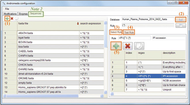
Configuration of Andromeda
-
3.
The uniqueness of peptide is related to the proteome database. In MaxQuant, a peptide is recognized as unique to a group of proteins (termed protein group) if on the entire proteome its sequence only occurs in this group.
-
4.
The inspection is crucial for cases where multiple peaks are detected, and consequently selection of the best peak may not be consistent across samples. To improve the performance of peak selection, Skyline also allows users to create custom advanced selection models and to utilize information from iRT retention time prediction of peptides.

References
Diamandis EP (2004) Mass spectrometry as a diagnostic and a cancer biomarker discovery tool: opportunities and potential limitations. Mol Cell Proteomics 3:367–378
Gstaiger M, Aebersold R (2009) Applying mass spectrometry-based proteomics to genetics, genomics and network biology. Nat Rev Genet 10:617–627
Ahrens CH, Brunner E, Qeli E et al (2010) Generating and navigating proteome maps using mass spectrometry. Nat Rev Mol Cell Biol 11:789–801
Aebersold R, Mann M (2003) Mass spectrometry-based proteomics. Nature 422:198–207
Domon B, Aebersold R (2006) Mass spectrometry and protein analysis. Science 312:212–217
Elias JE, Haas W, Faherty BK et al (2005) Comparative evaluation of mass spectrometry platforms used in large-scale proteomics investigations. Nat Methods 2:667–675
Oberg AL, Vitek O (2009) Statistical design of quantitative mass spectrometry-based proteomic experiments. J Proteome Res 8:2144–2156
Karpievitch YV, Polpitiya AD et al (2010) Liquid chromatography mass spectrometry-based proteomics: biological and technological aspects. Ann Appl Stat 4:1797–1823
Karpievitch Y, Stanley J, Taverner T et al (2009) A statistical framework for protein quantitation in bottom-up MS-based proteomics. Bioinformatics 25:2028–2034
Eng JK, Searle BC, Clauser KR et al (2011) A face in the crowd: recognizing peptides through database search. Mol Cell Proteomics 10:R111.009522
Pluskal T, Castillo S, Villar-Briones A et al (2010) MZmine 2: modular framework for processing, visualizing, and analyzing mass spectrometry-based molecular profile data. BMC Bioinformatics 11:395
Savitzky A, Golay MJE (1964) Smoothing and differentiation of data by simplified least squares procedures. Anal Chem 36:1627–1639
Jaitly N, Mayampurath A, Littlefield K et al (2009) Decon2LS: an open-source software package for automated processing and visualization of high resolution mass spectrometry data. BMC Bioinformatics 10:87
Sturm M, Bertsch A, Gropl C et al (2008) OpenMS—an open-source software framework for mass spectrometry. BMC Bioinformatics 9:163
Yu T, Park Y, Johnson JM et al (2009) apLCMS—adaptive processing of high-resolution LC/MS data. Bioinformatics 25:1930–1936
Coombes KR, Tsavachidis S, Morris JS et al (2005) Improved peak detection and quantification of mass spectrometry data acquired from surface-enhanced laser desorption and ionization by denoising spectra with the undecimated discrete wavelet transform. Proteomics 5:4107–4117
Du P, Kibbe WA, Lin SM (2006) Improved peak detection in mass spectrum by incorporating continuous wavelet transform-based pattern matching. Bioinformatics 22:2059–2065
Cox J, Mann M (2008) MaxQuant enables high peptide identification rates, individualized p.p.b.-range mass accuracies and proteome-wide protein quantification. Nat Biotechnol 26:1367–1372
Steen H, Mann M (2004) The abc’s (and xyz’s) of peptide sequencing. Nat Rev Mol Cell Biol 5:699–711
Zhang P, Li H, Wang H et al (2011) Peak tree: a new tool for multiscale hierarchical representation and peak detection of mass spectrometry data. IEEE/ACM Trans Comput Biol Bioinform 8:1054–1066
Kultima K, Nilsson A, Scholz B et al (2009) Development and evaluation of normalization methods for label-free relative quantification of endogenous peptides. Mol Cell Proteomics 8:2285–2295
Sysi-Aho M, Katajamaa M, Yetukuri L et al (2007) Normalization method for metabolomics data using optimal selection of multiple internal standards. BMC Bioinformatics 8:93
Callister SJ, Barry RC, Adkins JN et al (2006) Normalization approaches for removing systematic biases associated with mass spectrometry and label-free proteomics. J Proteome Res 5:277–286
Dunn WB, Broadhurst D, Begley P et al (2011) Procedures for large-scale metabolic profiling of serum and plasma using gas chromatography and liquid chromatography coupled to mass spectrometry. Nat Protoc 6:1060–1083
Cox J, Hein MY, Luber CA et al (2014) Accurate proteome-wide label-free quantification by delayed normalization and maximal peptide ratio extraction, termed MaxLFQ. Mol Cell Proteomics 13:2513–2526
Mann M, Kelleher NL (2008) Precision proteomics: the case for high resolution and high mass accuracy. Proc Natl Acad Sci U S A 105:18132–18138
Bellew M, Coram M, Fitzgibbon M et al (2006) A suite of algorithms for the comprehensive analysis of complex protein mixtures using high-resolution LC-MS. Bioinformatics 22:1902–1909
Mathias V, Sebastien Li-Thiao T, Hans-Michael K et al (2008) Alignment of LC-MS images, with applications to biomarker discovery and protein identification. Proteomics 8:650–672
Listgarten J, Emili A (2005) Statistical and computational methods for comparative proteomic profiling using liquid chromatography-tandem mass spectrometry. Mol Cell Proteomics 4:419–434
Tsai TH, Tadesse MG, Di Poto C et al (2013) Multi-profile Bayesian alignment model for LC-MS data analysis with integration of internal standards. Bioinformatics 29:2774–2780
Tsai TH, Tadesse MG, Wang Y et al (2013) Profile-based LC-MS data alignment—a Bayesian approach. IEEE/ACM Trans Comput Biol Bioinform 10:494–503
Fischer B, Grossmann J, Roth V et al (2006) Semi-supervised LC/MS alignment for differential proteomics. Bioinformatics 22:e132–e140
Jaffe JD, Mani DR, Leptos KC et al (2006) PEPPeR, a platform for experimental proteomic pattern recognition. Mol Cell Proteomics 5:1927–1941
Tuli L, Tsai TH, Varghese RS et al (2012) Using a spike-in experiment to evaluate analysis of LC-MS data. Proteome Sci 10:13
Cox J, Neuhauser N, Michalski A et al (2011) Andromeda: a peptide search engine integrated into the MaxQuant environment. J Proteome Res 10:1794–1805
Picotti P, Aebersold R (2012) Selected reaction monitoring-based proteomics: workflows, potential, pitfalls and future directions. Nat Methods 9:555–566
MacLean B, Tomazela DM, Shulman N et al (2010) Skyline: an open source document editor for creating and analyzing targeted proteomics experiments. Bioinformatics 26:966–968
Sherwood CA, Eastham A, Lee LW et al (2009) MaRiMba: a software application for spectral library-based MRM transition list assembly. J Proteome Res 8:4396–4405
Mead JA, Bianco L, Ottone V et al (2009) MRMaid, the web-based tool for designing multiple reaction monitoring (MRM) transitions. Mol Cell Proteomics 8:696–705
Lange V, Malmstrom JA, Didion J et al (2008) Targeted quantitative analysis of Streptococcus pyogenes virulence factors by multiple reaction monitoring. Mol Cell Proteomics 7:1489–1500
Martin DB, Holzman T, May D et al (2008) MRMer, an interactive open source and cross-platform system for data extraction and visualization of multiple reaction monitoring experiments. Mol Cell Proteomics 7:2270–2278
Acknowledgements
This work was supported by the NIH Grants R01CA143420 and R01GM086746.
Author information
Authors and Affiliations
Corresponding author
Editor information
Editors and Affiliations
Rights and permissions
Copyright information
© 2016 Springer Science+Business Media New York
About this protocol
Cite this protocol
Tsai, TH., Wang, M., Ressom, H.W. (2016). Preprocessing and Analysis of LC-MS-Based Proteomic Data. In: Jung, K. (eds) Statistical Analysis in Proteomics. Methods in Molecular Biology, vol 1362. Humana Press, New York, NY. https://doi.org/10.1007/978-1-4939-3106-4_3
Download citation
DOI: https://doi.org/10.1007/978-1-4939-3106-4_3
Publisher Name: Humana Press, New York, NY
Print ISBN: 978-1-4939-3105-7
Online ISBN: 978-1-4939-3106-4
eBook Packages: Springer Protocols