
Abstract
Computational methods and tools are nowadays widely applied for rational Metabolic Engineering approaches. However, what is still missing are clear advices on the right order of the application of these tools. The availability of genomic information for a large number of cellular systems especially requires the use of computers to store, analyze, and process knowledge of single enzymes, metabolic pathways, and cellular networks. The trend of integrating measured quantities for the metabolome, the transcriptome, and the proteome into mathematical models, combined with methods for the rational design of cellular networks, has led to the research field Systems Metabolic Engineering, a field that extends and amplifies the classical field of Metabolic Engineering. This chapter describes mathematical and computational approaches on the cellular and the process levels. In the Material section, modeling approaches and methods for model analysis are introduced, and the current state of the art is reviewed. In the Method section, we propose a protocol for efficiently combining various approaches for the optimal production of desired biotechnological products.
Access provided by CONRICYT – Journals CONACYT. Download protocol PDF
Keywords
- Constraint-based modelling
- Dynamic flux balance analysis
- Flux balance analysis
- In silico strain optimization
- Metabolic Engineering
- Metabolic models
- Stoichiometric analysis
- Succinate production
- Systems Metabolic Engineering
- Theoretical yields
1 Introduction
Computational methods and tools are nowadays widely applied for rational Metabolic Engineering approaches. The optimization of hydrocarbon and lipid production or degradation is one concrete example for the application of this tool and has already been applied successfully by a number of research groups [1–4]. Usually, a large amount of biological data is necessary for Metabolic Engineering. For example, the availability of genomic information for a large number of cellular systems especially requires the use of computers to store, analyze, and process knowledge of single enzymes, metabolic pathways, and cellular networks. The trend of integrating measured quantities for the metabolome, the transcriptome, and the proteome into mathematical models, combined with methods for the rational design of cellular networks, has led to the research field Systems Metabolic Engineering, a field that extends and amplifies the classical field of Metabolic Engineering. In recent years different views have become popular that describe the field (Fig. 1).

Views describing the field of Metabolic Engineering. Each view tackles the engineering problem of the efficient target production using different tools and focuses. This chapter describes theoretical tools used in the laboratory-based view
All views address a different question but have a common aim, namely, the efficient production of a target. Depending on the applied tools, methods, and researcher expertise, the cell-based view, the compound-driven view, or the laboratory-based view predominate. The cell-based view starts by exploring the capabilities of the cellular systems and modifies enzymes, pathway elements, or network elements to optimize the system [5]. Furthermore, the ease of genetic manipulation and cultivation of the cells is the driving force. The compound-based view [6] starts with the target component and asks how the component can be synthesized. The laboratory-based view distinguishes between experimental and theoretical approaches.
In the theoretical laboratory-based view, computational tools must perform diverse tasks to support the optimization of cellular systems with respect to the production of desired compounds. Three main tasks can be identified: search for information in genomic and metabolic databases, description and integration of experimental data in mathematical models, and application of optimization strategies to improve single enzymes, to design pathways and networks, and to construct new cellular circuits.
For the first of these tasks, databases like KEGG [7], EcoCyc [8] or Brenda [9] provide information about compounds, reactions, and networks for various cellular systems. Moreover, kinetic information, that is, information on the temporal behavior of enzymes, can also be found. In general, the information is very detailed, ranging from the chemical structure of compounds and promoter and ribosome sequences to pathway information. In this way, databases support all strategies for modification of cellular systems. The setup and the analysis of mathematical models are further pillars in Systems Metabolic Engineering. Such models are helpful in two ways: first, they integrate what we know of a system in terms of mathematical equations. Since these equations are based on physical and chemical laws, models are used to check the consistency of the knowledge and thereby allow researchers to detect missing or incorrect items. Second, quantitative models, that is, models that are validated with quantitative experimental data, have potential for prediction. The chance to make predictions about conditions that were not used for model validation opens possibilities for model-based modifications such as optimization of cellular properties. Optimization itself plays the most important role in Systems Metabolic Engineering and is used not only on the cellular level but also on the process level.
When optimizing the metabolic system with respect to the production of a target, there are two possible cases. Figure 2 shows that either the target is already inherently produced by the host cell (case A), or a noninherent pathway has to be inserted (case B). In case A, a metabolite is often produced only at a low specific rate r, while the organism is growing at a high growth rate (Fig. 2a, left). The aim is to construct a strain with a higher specific production rate. Caused by a reorganization of the available resources, a lower growth rate results (Fig. 2a, right). If the target is not produced by the strain inherently (Fig. 2b, left), heterologous DNA information should be introduced into the strain. When new enzymes are expressed and the desired product is built, it is expected that the growth rate also decreases (Fig. 2b, right).

Resource usage in two different cases. The circles represent the available cellular resources and how they are used in different situations: (a) the target is already produced inherently by the cell (left). Optimization of this metabolic system results in a rearrangement of the resources (right). (b) If the target is not produced naturally (left), a noninherent pathway has to be introduced. This also causes a reorganization of the cellular metabolism. Here, the plasmids represent the heterologous DNA introduced into the host cell (right)
This chapter describes mathematical and computational approaches on the cellular and the process level. In the Material section, modeling approaches and methods for model analysis are introduced, and the current state of the art is reviewed. In the Method section, we propose a protocol for efficiently combining various approaches for the optimal production of desired biotechnological products.
2 Materials
Commonly used materials for computer-guided Metabolic Engineering include metabolic reconstructions, model equations for the cellular reaction network and for the bioreactor system, experimental data, and software. The last category included solvers, computing environments, and/or programming languages.
2.1 Metabolic Reconstruction
A genome-scale metabolic reconstruction is a mathematical representation of the metabolism of a living cell. It is typically made up of the stoichiometry of all known reactions that take place inside an organism and the enzymes and genes associated with that reaction. Additionally, a reaction accounting for biomass generation [Eq. (1)] which is based on the biomass composition of that microorganism and an estimation for growth- (GAM) and nongrowth-associated energy requirements (NGAM) are also important components of the metabolic reconstruction. The concept of GAM and NGAM for the description of the energetics of bacterial cell growth was first mathematically formalized by Pirt [10]. GAM accounts for the energy needed to synthetize macromolecules (DNA, RNA, lipids, etc.) necessary for cell growth, while NGAM refers to the energy consumed for functions other than production of new cellular material.
High-quality genome-scale metabolic reconstructions for many industrially important microorganisms are freely available in public repositories (http://sbrg.ucsd.edu/Downloads). The methods for building those reconstructions are also well established [11]. Curated metabolic models can be used in constraint-based modeling approaches for the estimation of metabolic capabilities of the cell, hypothesis testing and generation, and Metabolic Engineering [12].
The scope and coverage of the metabolic reconstructions can vary substantially. Table 1 shows the evolution of the genome-scale metabolic reconstruction of Escherichia coli (E. coli) over the last decade [13, 14].
During this period of time, many new reactions have been introduced, and some others have been updated based on newly available biochemical knowledge. The selection of a specific metabolic reconstruction depends on the aim of the simulations to be performed. However, it is highly recommended to start with a small version (core model) of the metabolic network of interest. This allows a better understanding of the methods used while keeping an overview of the results obtained.
2.2 Model Equations
In this section, mathematical equations describing the dynamics of metabolite concentration inside the cell and the reactor are discussed. The idealized case of perfect mixing, in which no spatial concentration gradients are considered, is assumed for the reactor and the cell. The mass balance for the intracellular metabolites is formulated for an average cell, which is assumed to be representative of the whole cell population.
2.2.1 Intracellular Reaction Networks and Constraint-Based Modeling
Biochemical reactions taking place in a cell can be generically written as:
γ ij are stoichiometric coefficients and A, B, X, D, F, and G represent network components. The corresponding mass balance for each intracellular component reads:
where C A is the concentration of component A in the cell [mmol gDW−1] and r i represents the reaction rate of the reaction i [mmol gDW−1 h−1]. Note that the stoichiometric coefficients γ ij are contained in the so-called stoichiometric matrix S. Therefore, the matrix S itself can be used for the intracellular mass balance formulation:
where r is a flux vector, μ is the growth rate, and c is the concentration vector, which contains the concentrations for all components (C A , C B , etc.). In most cases, the dilution term (μ c) is small in comparison to the intracellular fluxes, and the equation can be simplified as follows:
The steady state is a special case in which no temporal change of the intracellular concentrations is considered. This can be mathematically expressed as:
The equation above does not have a unique solution. The number of variables (reactions of the metabolic network) is usually much larger than the number of equations (metabolites), and measured reaction fluxes are normally scarce. Additional constraints can be applied to further reduce the number of allowable flux distributions [18]. Limits on the range of individual flux values can be used for this purpose; thermodynamic constraints [19] expressed as the directionality of a given reaction [16] can thus be used by setting one of the boundaries for that reaction to zero if the reaction is irreversible. In a similar way, maximum flux values can be estimated based on enzymatic capacity limitations [20], or for the case of exchange reactions, measured maximal uptake rates can be used (Sect. 3.3). Regulation of gene expression can also be considered in cases where the regulatory effects have a great influence on cellular behavior [21]. Usually, these constraints are not sufficient to reduce the solution space to a single solution. Therefore, linear programming methods are used to find a flux distribution that satisfies the problem:
where Z is the objective function to be maximized (see Sect. 3.4.1), r is the flux vector, lb and ub are the lower and upper flux boundaries, respectively, and S is the stoichiometric matrix of the metabolic network. A reaction describing biomass generation [Eq. (1)] has been successfully used as an adequate objective function for predicting in vivo cellular behavior [22–24]. The above-explained approach is known as flux balance analysis (FBA) and is the most commonly used method for simulating the cellular phenotype.
2.2.2 Model for Bioreactor System
A generic mass balance equation for any component in a bioreactor can verbally be formulated as:
The term “mass converted in the system” refers to the catalytic activity of living cells. The equation is used to formulate mass balance equations for the volume of the reactor, for the biomass, and for the components in the liquid phase of the reactor. Table 2 gives an overview of the variables used. For a more complete description, refer to Kremling [25].
2.2.2.1 Volume of the Bioreactor
The dynamics of the reactor volume can be described by:
If ρ is assumed to be constant and since \( {m}_R={V}_R\rho \):
2.2.2.2 Biomass
For modeling of the biomass, it is assumed that the feed contains no cells. Cell recirculation is also not considered. The mass balance for the biomass reads:
The growth rate μ can be typically expressed as a function of the substrate uptake rate and the biomass yield: \( \mu ={Y}_{X/S\ }\ {r}_{Si}^e\ {w}_{Si} \). For convenience, the biomass dynamics are now expressed in terms of biomass concentration. This is done by expressing the biomass in the reactor [g] as a function of the biomass concentration [g l−1] and the reactor volume [l]:
Substituting Eqs. (12) and (10) into Eq. (11) and solving for biomass concentration lead to:
2.2.2.3 Components in the Liquid Phase
The mass balance for substances (substrates/products) in the liquid phase is derived in a similar way as for the biomass. The mass balance for the component i is shown in Eq. (14). In this case, exchange reactions r e Si between the cell and culture media have to be considered. A positive sign is used for products secreted by the cell, whereas a negative sign precedes r e Si for substrates absorbed by the cell.
The mass balance equations derived for biomass, reactor volume, and components in the liquid phase can be used to describe the dynamics of a continuous (\( {q}_{\mathrm{in},j}\ne 0 \); \( {q}_{\mathrm{out}}\ne 0 \)), a batch (\( {q}_{\mathrm{in},j}={q}_{\mathrm{out}}=0 \)), or a fed-batch process (\( {q}_{\mathrm{in},j}\ne 0 \), \( {q}_{\mathrm{out}}=0 \)).
2.3 Experimental Data
With the development of high-throughput technologies, it is currently possible to produce large amounts of experimental data to characterize the proteome, genome, metabolome, and transcriptome of a microorganism under specific conditions. This allows a system-wide analysis of the cell response to genetic perturbations and operating conditions in the bioreactor, such as glucose and oxygen concentrations. Genome-scale reconstructions provide a suitable framework for the analysis and integration of these large datasets. To this end, many approaches have been developed over the last years. Hyduke [26] and Kim and Lun [27] provide a good overview of the possibilities of integrating omics data with genome-scale models. A recent multi-scale, genome-wide model of E. coli [28] represents an illustrative example of integrative modeling. The model incorporates the gene expression data of 4,189 genes in 2,198 conditions, transcriptional regulation, signal transduction, and metabolic pathways.
If the abovementioned high-throughput measurements are not readily available for the organism of interest, insights into the metabolism of wild-type and mutant strains can be gained using simple experiments. For instance, measurements of the time course of concentrations of extracellular metabolites can be used to determine cell-specific uptake and production rates [29]. The resulting rates can then be used as constraints for the corresponding exchange reactions used to reduce the solution space of the metabolic model describing the metabolism of the cell (see Sects. 2.2.1 and 3.3).
2.4 Software
Table 3 summarizes some commonly used software packages that support the calculations necessary for Metabolic Engineering. Some tools, like YANA, are stand-alone and need no extra software for their operation. Some others, like the widely used COBRA Toolbox, are packages that require previous installation of a specific platform (Matlab or Python) and a solver. Python + COBRApy + Glpk represent high-quality, free, open-source options and are recommended if a Matlab license is not available. Gurobi offers a free academic license and is therefore a good option when performing quadratic or quadratically constrained programming.
2.5 Next-Generation Models for Metabolic Engineering
Metabolic processes taking place in the cell are strictly coordinated by highly interconnected, complex, and sometimes intricate networks. The activity level of a specific enzyme in the cell can be regulated at the transcription/translation level as well as by using posttranslational modifications, which in turn are coordinated by signaling networks. Thus, observable cellular behavior results from a complex interplay of multiple cellular networks. First attempts to integrate metabolic reconstructions into additional networks have already been made by many research groups [28, 35–37].
A current example is the development of the first model, which aims to integrate metabolism and gene expression (ME-Models) for E. coli [35, 36]. ME-Models extend the prediction capabilities of the traditional metabolic models (M-models), allowing, for instance, the assessment of the metabolic burden observed in cells expressing large engineered pathways. Thus, with ME-Models, engineering strategies to overcome the metabolic burden can be better explored. With the addition of further details and the refining of the ME-Models [37], the dimension of the stoichiometric matrix grows to a computationally challenging magnitude. The great scope of the ME-Models encompasses not only their tractability but also their analysis of the simulation results. As an alternative to these detailed models, a mechanistic ODE-model (compartment model) that describes transcription and translation [38, 39] of gene pools can be coupled with a metabolic model. The application of such a compartment model that describes the relationship between growth rate and the content of RNA, DNA, and bulk protein, and additionally accounts for the amount of free and bounded ribosomes, improves the prediction capabilities of the extended model while keeping it tractable.
3 Methods
Here, we propose a five-step Metabolic Engineering strategy to achieve the optimal production of a target molecule in a selected host microorganism. Figure 3 summarizes the main phases of the strategy and shows the associated chapters, in which each step is explained in detail.

Five-step Metabolic Engineering strategy. Light gray symbols represent methods, while the dark gray symbols represent the result of these methods. Material is an input in different stages but is shown only for the first method. The sections of this book chapter are represented by the numbers
In the first step, a theoretical characterization of the capabilities of the strain is performed. Moreover, optimal pathway configuration and medium composition are estimated for the production of the target. For this purpose, an adequate metabolic model is analyzed using flux balance analysis (FBA) and its extensions. In the second step, in silico strain optimization algorithms are used to predict gene/reaction deletions that redirect the carbon flow toward the production pathways. In the third and fourth steps, experimental data is analyzed and integrated. The comparison of the estimated intracellular flux pattern of the wild-type and mutant strains can be used to evaluate the effect of genetic manipulations on the improvement of product yield. In the last step, the performance of the engineered strains in a bioreactor is assessed, and by selecting adequate process conditions, improvements of productivity and final titer are achieved. Dynamic flux balance analysis plays a central role in this last step.
3.1 Theoretical Product Yields and Pathways
Even before experimental data for the strain to be engineered is available (Sect. 2.3), a pure theoretical characterization of the metabolic system capabilities can be performed using a suitable metabolic reconstruction. The methods discussed in this section include:
-
Theoretical product yields: can be used as an indicator for the performance potential of the wild-type/mutant strains under different conditions
-
Optimal pathway configuration: facilitates decisions about which pathway or pathway combinations have to be used to optimally produce the target molecule
-
Optimal medium composition: guides the selection of the real medium composition by showing which substrates have a positive impact on product yield
3.1.1 Calculation of the Theoretical Product Yields
A metabolic reconstruction, specific for the host strain used, is necessary to calculate the maximal theoretical product yield supported by the host microorganism. The theoretical product yield is a function of the thermodynamic, stoichiometric, and physiological constraints considered when performing the calculations. The procedure for calculating the maximal theoretical yield is explained for the production of succinate in E. coli as a case study.
-
1.
Choose a metabolic reconstruction of E. coli. See Table 1.
-
2.
Set the production of succinate as an objective function. Here one can choose between selecting an existing reaction and adding a new one to the model. In case of the E. coli core model, the reaction SUCCt3 (succinate transport out via proton antiport) is a good candidate for the objective function. If one decides to add a new reaction, it should be of the form “succ[c] →.”
-
3.
Define the medium composition. This is done by modifying the upper and lower limits of the exchange reactions. For this specific example, we will assume that glucose is the sole carbon source.
-
4.
Add additional constraints to the model (gene deletions, growth rate, GAM value, etc.).
-
5.
Assume an arbitrary uptake rate for glucose (if no experimental measurements are available) and solve the linear programming problem using an adequate solver (see Note 1).
-
6.
The resulting flux distribution should now be scaled to the input flux of glucose in order to get the value of the maximal theoretical yield (see Note 2).
The COBRA Toolbox provides a set of functions that facilitate the execution of all these steps with only a few code lines (Table 4). For a detailed explanation of these functions, refer to the COBRA Protocol [30].
The effect of imposing different constraints on the maximal theoretical yield is illustrated in Fig. 4. Aerobic and anaerobic cultivations are considered with glucose as the sole carbon source. Three situations are analyzed: two cases in which growth is not considered and one case in which the growth rate has an arbitrary value of 0.35 h−1. The yield values reported in Fig. 4 represent the limits for the metabolic system under these conditions. No higher yields are possible as long as the metabolic network is not modified (addition or stoichiometry modification of reactions). It can be seen that growth has a negative effect on the maximal theoretical yield. This is a logical consequence if the biomass is considered as an additional product that has to be synthetized by the metabolic system. The more biomass is produced, the less carbon will be available for the production of the target biomolecule. Additionally, Fig. 4 shows that for the succinate production in E. coli, a maximal theoretical carbon yield of one can only be reached under aerobic conditions. This is further analyzed in Sect. 3.1.3.

Effect of constraints on theoretical yields: aerobic and anaerobic cultivations are considered with glucose as sole carbon source for the production of succinate in E. coli. Three different situations are analyzed: two cases in which growth is not considered (μ = 0) and one case with a growth rate of 0.35 h−1. The maximal possible yields are calculated for each situation, and the results are presented as molar (left) and carbon (right) yields. A carbon yield of 1 (equivalent to a molar yield of 1.5) indicates that the metabolic system is capable of converting all supplied carbon atoms into product
3.1.2 Determining an Optimal Pathway Configuration Using Stoichiometric Analysis
Many bio-products can be produced using different biochemical routes. These routes can occur naturally either in the host strain itself (native pathways) or in other organisms (heterologous pathway), or they can be synthetically generated. Metabolic engineers are thus often confronted with the task of selecting the best pathway configuration to be engineered in the host cell. Pathway configuration refers here to the situation of using pathway A, pathway B, or a combination of both for the biosynthesis of a target product R (Fig. 5a). This choice should be made considering many aspects, e.g., energy, cofactor, and reduction equivalent consumption. Curated metabolic models can be used to guide the selection process of the pathway configuration with the best performance index: molar and carbon yield are commonly used performance indices when comparing pathways (see Note 3). The procedure of finding a pathway configuration that reaches the maximal performance index is explained using a hypothetical case study, in which pathway A and pathway B lead to the formation of the product R. In the hypothetical case study, pathway A is a native pathway, while pathway B is a heterologous one.

(a) Pathway configuration for wild-type and engineered but suboptimal strain: two different situations are shown. The left panel shows the wild type, in which the substrate flows only into the native pathway A (f = 1). The native pathway A consumes one molecule of ATP and NAD(P)H. In the central panel, pathway B is added to the wild-type strain. The heterologous pathway B produces one molecule of ATP and NAD(P)H. In this engineered strain, 10% of the carbon flows into the native pathway A and the rest into pathway B (f = 0.1). This pathway configuration is not optimal. Equations describing the carbon distribution are shown in the right panel. r A and r B represent the rates through the first reaction of pathways A and B, respectively. A f-value of one means that all of the carbon flows into pathway A. (b) Simulation of different pathway configurations. The maximal performance index is reached when 37% of the substrate flows into the native pathway A (f = 0.37). The synergy observed arises from the dynamics of ATP and NADPH between the two pathways
-
1.
Identify the different pathways that lead to the target bio-product formation.
-
2.
Incorporate new biochemical routes, if necessary.
-
3.
Identify the common branch point of the pathways. See Fig. 5a.
-
4.
Use the flux ratio between pathway A and B to specify the flux through each pathway. Use the variables x and f as shown in Fig. 5a for this propose.
-
5.
Add the marked equation in Fig. 5a as a new constraint in the stoichiometric matrix. The coefficients are x and −1 for the first reaction of pathways A and B, respectively.
-
6.
Calculate the maximal theoretical performance index for different pathway configurations, i.e., different values of flux ratio x or flux fraction f. Note that the variable f (flux fraction) can only take values between 0 and 1, while the flux ratio ranges from 0 to infinity.
-
7.
Select the optimal pathway configuration from the simulation results. See Fig. 5b.
The effect of the pathway configuration on the selected performance index, in this case molar yield, is illustrated in Fig. 5b. In this hypothetical case study, the native pathway A has a lower performance index than the heterologous pathway B. However, the system only becomes optimal when both pathways are expressed in a fraction of f = 0.37. Shen and Liao [40] experimentally proved the validity of the approach described above when engineering E. coli for the production of 1-propanol. They observed an improvement of the 1-propanol yield of 30–50% when expressing both the heterologous citramalate pathway and the native threonine pathway for the production of the 1-propanol intermediate 2-ketobutyrate, compared to the yield when using only one pathway. The synergy observed was in good agreement with the predictions made with the approach explained above.
3.1.3 Estimation of the Culture Medium Composition
Which are the optimal substrates for the production of a desired target molecule? Should the production be performed under aerobic or anaerobic conditions? Can the totality of the assimilated carbon be transformed into product by the metabolic system in its actual configuration? Finding the answers to these and similar questions can be challenging and requires a great experimental effort. However, when dealing with these issues, a sensitivity analysis of the metabolic model of the strain being engineered can be helpful. The general procedure is illustrated again, using the example of succinate production in E. coli.
-
1.
Select an adequate metabolic reconstruction of the analyzed strain. See Sect. 2.1.
-
2.
Define a base model. This model will represent the starting conditions for the sensitivity analysis. In the concrete case of the succinate production in E. coli, the starting conditions correspond to no carbon source and anaerobic conditions.
-
3.
Define a biologically meaningful range for each analyzed exchange reaction. For instance, the glucose uptake rate was assumed to have a maximal value of 18 mmol gDW−1 h−1.
-
4.
Vary the lower limit of an arbitrary exchange reaction, inside of the predefined range, in order to permit the system to absorb the corresponding compound.
-
5.
Calculate the maximal value of the desired performance index. See Sect. 3.1.1.
-
6.
Repeat steps 4 to 5 until all exchange reactions of interest are analyzed.
-
7.
Sort the results in a table and make decisions about what compound should be added to the culture medium (base model) in order to improve the performance index.
-
8.
If the desired value for the performance index is not reached after modifying the base model, repeat steps 1–7 until the desired performance is accomplished.
The production of succinate in E. coli is an extensively studied process. Therefore it is a good case study to show the utility of the approach explained above in guiding the selection of medium composition. Encouraging steps toward an engineered E. coli strain with high yield, productivity, and titer have been made. Most of the work reported to enhance the succinate production has been performed under anaerobic conditions [41–43]. Interestingly, a simple sensitivity analysis shows (Table 5b) that the maximal theoretical carbon yield can only be reached under aerobic conditions. E. coli mutants, which produce succinate under aerobic conditions, and a theoretically designed high-performance aerobic strain have been reported [44, 45]. The sensitivity analysis can also guide the development of an anaerobic cultivation process. It shows that the addition of carbon dioxide to the system has a positive effect on the maximal yield. It is therefore logical to use a carbon dioxide atmosphere in anaerobic cultivations. This fact has been identified and used by many research groups [46–48].
3.2 In Silico Strain Optimization
Genome-scale reconstructions of metabolism have been used for over a decade now to predict genetic modifications that improve the product yield and production performance of the engineered production strains. Some manipulation strategies that can be explored in silico are listed in Table 6. A more extensive overview of these methods can be found in [5]. The first algorithms for in silico strain design permit us to predict the effect of reaction knockouts, that is, they consider the effect that reaction deletions have on the metabolic network and product yield. Predicting the up- and downregulation of reactions represents an extension of these first algorithms. Additionally, if gene-protein reaction (GPR) mappings are available for the metabolic system being analyzed, algorithms that only predict gene knockouts can be used and should be preferred, as exactly these modifications will later be experimentally implemented in the real biological systems.
The general procedure used to perform in silico strain optimization is explained using the metabolic network shown in Fig. 6, as described by Kremling [25]. X and P represent the biomass and the target product, respectively. P, C, and B are intermediates. In this example, the synthesis of P is coupled to growth (X).

(a) Hypothetical metabolic network for the production of P and X. (b) The network consists of seven reactions. A, B, C, and D are intermediates. (c) Two reaction knockouts – r 3 and r 7 – are necessary to maximize the production of biomass and at the same time product P [25]
-
1.
Set up the metabolic model or choose an existing genome-scale metabolic reconstruction.
-
2.
Identify the reactions that contribute to the production of the target molecules. In this example the reactions r 4 and r 6 synthetize the product P, and the reactions r 2, r 3, r 5, and r 6 contribute to the formation of biomass.
-
3.
Define the objective functions: Z 1 = f(r 4,r 6) and Z 2 = f(r 2,r 3,r 5,r 6) for product and biomass, respectively.
-
4.
Select the set of reactions that can be deleted from the network.
-
5.
Determine the number, n, of reactions to be knocked out. The computing time required to find a solution depends on the algorithm used and can increase exponentially or linearly with the total number of knockouts in the mutant strain.
-
6.
Select a strain optimization algorithm (Table 6) and perform the simulation. It is strongly recommended to use more than one algorithm to perform the in silico strain optimization. Since each algorithm examines the solution space in a different way (local/global search, one path/multiple path), finding different solutions is to be expected. OptKnock is a good starting point and is already implemented in the COBRA Toolbox.
-
7.
Analyze the predicted gene deletions in respect to biological consistence and select the best option to be experimentally implemented. Note that due to inherent inaccuracies in the metabolic model, not all predicted mutants are biologically feasible. Further genetic modifications might be necessary in order to obtain the optimal flux distribution that maximizes the product yield. A good example for this situation is the design of a high-performance aerobic E. coli strain for the succinate production, in which additional genetic modifications are necessary to obtain the optimal flux distribution predicted by EMILiO [44].
In the case of the network shown in Fig. 6, only two reaction knockouts are sufficient to maximize the reaction flux through the product and biomass. The network was optimized using the OptKnock algorithm. Reaction two to reaction seven conform the set of reactions that can be deleted. The calculation time required was 0.005 s.
3.3 Analysis of Experimental Data
For analyzing and optimizing a host strain, substrate uptake rates and product excretion rates must be determined to calculate the complete flux distribution. The rates measured can be used to identify bottlenecks as well as to confirm engineering success. Basically, the more metabolic data are available, the more precise and better is the evaluation of the fluxes.
Biomass and substrate concentrations especially are easily measurable during an experiment, and commercial kits for accessing them are often available. In many laboratories, measurement tools like HPLC to quantify the cellular output in the form of metabolites have already been established. In an open system, such as the standard shaking flask, it is not possible to close the mass balance because of the impossibility of determining all carbon fluxes in the system (e.g., CO2 that is produced by the cells). Therefore, a bioreactor system and an exhaust gas analyzing system are recommended.
After pre-culturing, the strain of interest should be inoculated in a defined minimal medium with a carbon source of interest. According to the fermentation strategy, either a feeding strategy or a batch cultivation with a specific initial concentration of the carbon source can be applied. Substrate feeding has to be included in the mathematical analysis as described in 2.2.2. The specific uptake and formation rates are determined depending on the corresponding time course data for the metabolite concentrations in the bioreactor system. To determine all relevant rates, data for all metabolites and for cell dry mass have to be taken from the same time frame and growth phase as shown in the gray-shaded area in Fig. 7a.

Fictive data for strain performance during a production process (a). The measured optical density increases with rising biomass (b). Graph c shows the logarithmic optical density in the exponential phase against time. Substrate concentration (d) and product concentration (e) are plotted with respect to the cell dry weight. To evaluate the respective rates, concentrations are related to biomass formation. Therefore, equations of the contemplated gradients are necessary. The rate is equal to the slope of the straight line multiplied by the growth rate. Corresponding rates have to be analyzed in the same time frame and growth phase (gray shaded). A high coefficient of correlation R 2 is required to obtain conclusive results
As the rates should be normalized to the cell dry mass (DW), as a first step it is useful to correlate the measured optical density (OD) with the biomass (Fig. 7b). If there is no DW available, the OD can also be used as a proxy for biomass. In order to correlate substrate uptake and product formation rates, it is important to always use the same parameters (wavelength, growth stage, medium, etc.). At least three biological replicates should be measured to minimize the standard deviation of the measurement.
The biomass formation, also known as specific growth rate μ, is one particular case of formation rate. It can be determined directly from the slope of the measured logarithmic OD curve. Due to the (linear) correlation between OD and biomass concentration (Fig. 7b), the slope of the data points in the chosen interval is equal to the growth rate μ [Fig. 7c, Eq. (15)].
Metabolic rates have to be determined from the extracellular time course data of substance depletion or accumulation \( \frac{d{c}_{si}}{dt} \) that has to be related to the currently measured biomass concentration c B [Eq. (16)]. Uptake and formation rates r for a substance S not only correspond to the respective time point of the measurement but also to the already generated biomass c Bt [29]. The temporal alteration of biomass [Eq. (15)] has to be linked to the uptake or formation rate [Eq. (16)] to analyze those rates:
In order to calculate the substrate uptake rate as well as the product formation rate, the according concentration has to be plotted against the corresponding biomass (Fig. 7d and e). The slope \( \frac{d{c}_{si}}{d{c}_B} \) multiplied by the growth rate μ gives the respective rate [Eq. (16)] (see Note 4).
3.4 Estimation of the In Vivo Flux Distribution
First of all, measured rates can be fed into the already established metabolic model to restrict the solution space (Fig. 8). Additionally, to provide realistic flux estimations, an objective function and an adjusted value for GAM (see below) are included in the calculations.

In a comprehensive model, there are more unknown variables than equations. For defining a range of solutions, some constrains have to be given [11]. Additionally, a suitable objective function concerning the model output is required to compute an optimal network state and a resulting flux distribution [14]
3.4.1 Selecting an Adequate Objective Function
The most common assumption is that microbial cells maximize their growth [54]. For this reason biomass production is a frequently used objective function. However, depending on the growth phase, different objective functions as summarized in [54] are possible. So, in some cases it will be advantageous to combine a number of objective functions to restrict the solution space. If there is no growth, the energetic efficiency could be optimized instead of biomass yield. In this case the objective function would be the ATP yield. Another approach is to minimize the substrate consumption or the required number of reaction steps.
3.4.2 Calculation of Growth-Associated Maintenance (GAM)
Energy has to be considered for growth prediction. Cells have a specific energy requirement for maintenance metabolism [10]. This rate is defined as nongrowth-associated maintenance energy (NGAM) [14]. The yield of substrate uptake necessary for the resulting growth is defined as growth-associated maintenance metabolism (GAM) [14]. The available energy is specified with respect to the ATP concentration in order to meet different substrate compositions. The following steps need to be completed to calculate specific GAM values:
-
1.
Determine growth rate and substrate uptake rates of the analyzed strain from different experimental setups (here named as setups 1–5) with various growth rates (e.g., adjusted by dilution rate in a continuous culture using a chemostat [11] (Fig. 9a)).
Fig. 9 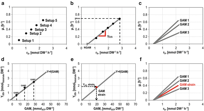
The strain of interest can be analyzed by considering different growth rates and substrate uptake yields under various setups (a, b). Theoretical strain behavior with fixed GAM values has to be computed (c) to create the Y X/S to GAM ratio (d). From this correlation the GAM of the strain can be determined (e). The yield of the substrate with respect to the growth rate can be compared to the performance of other strains (f), and growth rates can be predicted
-
2.
Compute the slope of the linear growth rate/substrate uptake rate correlation between \( \mu =0 \) and μ max (Fig. 9b).
-
3.
Calculate, with the help of the already available stoichiometric model, different theoretical yields Y X/S under different theoretical GAMs (here named GAM1–GAM3) (Fig. 9c) as described above (Sect. 3.1.1). The strain-specific NGAM value is assumed to be the same.
-
4.
After correlation of the used theoretical GAMs (here again GAM1–GAM3) with calculated yield Y X/S (Fig. 9d), the theoretical GAM out of the interpolated experimental data (Fig. 9b) can be read out as shown in Fig. 9e.
-
5.
Depending on the model, wild-type E. coli strains have a GAM around 60 mmolATP gDW−1 h−1 [16]. Mutants with an altered network structure will show a different behavior, and growth yields can be compared (Fig. 9f).
-
6.
The existing model can be adapted to be strain specific with the experimentally determined GAM. For the modeled strain, it is possible to predict growth rate and flux distributions for a given substrate uptake as well as vice versa.

The value for NGAM can be calculated as described in Sect. 3.1.1 by setting ATP as an objective function and measured q S NGAM as input (Fig. 9b).
3.4.3 Reconstructing In Vivo Flux Distributions
The strain performance has to be recorded under various conditions and experimental setups with different growth rates to determine flux distributions. Flux balance analysis enables the calculation of the flux through the metabolic network of the cell (see above Sect. 3.1.1). For many organisms, these networks are already available online. It is possible to reconstruct the flux distribution in a microbial cell based on metabolic reconstructions in the systems biology markup language (SMBL) format available online with the help of the COBRA Toolbox [30]. This toolbox allows the visualization of the actual fluxes and offers us the opportunity to compare fluxes in mutant strains with wild-type flux distributions (see Note 5).
As shown in Fig. 10a, many rates in the E. coli core model are not available (thin arrows). It is possible to calculate the carbon flux in silico by setting the measured uptake and excretion rates as additional constraints. Figure 10b shows a hypothetical flux distribution through the network. Setting the hypothetical flux D–E to zero (e.g., by a mutation) results in a measurable shift in the production rate of metabolite I. If the predicted flux distributions are not congruent to the actual measured rates, it is an indication that regulatory interactions or further pathways are missing in the model.

Metabolic data can only partially be determined via experimental setups. As shown in a schematic cell with metabolites A–I, experimental measured rates (thick arrows) have to be supplemented by in silico calculated rates (thin arrows) for wild type and mutants to determine the complete flux distribution (a). Dark numbers in (b) represent the actual flux rates. A modification in the network, for example, the flux \( \mathbf{D}\to \mathbf{E} \) is set to zero, results in an altered flux distribution as shown in (b). New rates are depicted in light gray
The presentation of metabolic networks is realized via graphical visualization of subnetworks. The output generated by Matlab enables a comparison of flux rates as shown in Fig. 10b. Maps from different metabolic pathways are available in BiGG knowledge base [55]. To create the image it is necessary to load the chosen map of interest into Matlab and draw it as a Matlab figure. This can be realized with only a few commands [30].
The stoichiometric matrix has to be modified to adapt the reconstruction to mutant strains proposed via in silico strain optimization. To get an idea of the most probable solution, the solution space of the mutant could be analyzed using the MOMA method, which is the minimization of metabolic adjustment [56]. This theory is based on the assumption that the “fitness” of the wild type has evolved over millions of years and represents the optimal metabolic state. This kind of pressure is not present for genetically modified organisms, which means that they probably do not possess the optimal growth configuration [56]. Caused by this, the most realistic flux distribution is the one derived from the solution space which contains the minimal distance to the wild-type flux distribution.
3.5 Assessing and Improving the Performance of Engineered Strains in a Bioreactor
The goal of the algorithms for strain optimization discussed in Sect. 3.2 is the redesign of the host metabolic network to maximize the yield of a target molecule while simultaneously supporting growth. This approach does not explicitly take into account the subsequent utilization of the engineered strain in a bioprocess, and consequently, the selected strain might not be optimal from an economical/operational point of view. The solution to this problem can be addressed in two different ways. The first approach considers criteria related to bioprocess design in the early stages of strain design. This can be done by combining existing in silico strain optimization algorithms with dynamic flux balance analysis [23, 57, 58] to optimize yield (Y), titer (T), and productivity (P) in a balanced fashion. Zhuang [59] presented a Dynamic Strain Scanning Optimization (DySScO) strategy that uses this rationale to produce strains that balance the product yield, titer, and productivity. DySScO searches for a strain design that maximizes a user-defined metric of the form: Z = f(Y, T, P). The second approach consists of decoupling the production of the target molecule from growth. The production process is thus divided into two phases. In the first phase, biomass is produced at a high rate and no production occurs. The second stage is characterized by low to no growth and production of the target chemical. The switching time from the growth phase to production has a high impact on the overall process performance.
Irrespective of the approach used, dynamic flux balance analysis (dFBA) has a central role in assessing and improving the performance of engineered strains in a bioreactor. dFBA combines both the process dynamics with the metabolic network, thus allowing the simulation of concentration profiles and flux distributions over time in the reactor and the cell, respectively. Shown here is the general procedure for performing a dFBA simulation with the COBRA Toolbox. Moreover, the utility of dFBA is illustrated with a case study.
-
1.
Select a metabolic reconstruction and perform the necessary adjustment of the network (gene/reaction deletions, new pathways) in order to describe the metabolism of the strain studied. See Note 6 .
-
2.
Specify values for strain-specific parameters. This refers to substrate uptake and production rates, maximum growth rate, product inhibition, etc. These values can be taken from the literature or correspond to experimental measurements.
-
3.
Define initial values for process-specific parameters. This refers to mode of operation (batch, fed batch), initial concentration of biomass and substrates, duration of the process, maximal reactor volume and feeding strategy (continuous substrate feeding, substrate pulses), time point of induction, etc.
-
4.
Perform a dFBA simulation and determine values for yield, titer, and productivity.
-
5.
Repeat steps 3 to 4 with a modified set of process-specific parameters until the desired performance for yield, titer, and productivity is reached. Alternatively, an optimization algorithm can be used to find the set of optimal process-specific parameters that maximize yield, titer, and productivity.
The procedure explained above will, in the following, be used to study a hypothetical case for which experimental data is available. The production system consists of a strain carrying an inducible plasmid, which expresses heterologous enzymes necessary to synthetize some product R. In this hypothetical experiment, cells were cultivated until a defined optical density was reached, and then the synthesis of R was induced. The effect of varying the time point of induction on the yield, productivity, and titer will be analyzed. Figure 11 shows the experimentally obtained concentration profiles of biomass, glucose, and product inside the bioreactor over time. As can be concluded from the glucose concentration profile in Fig. 11 (circles, middle plot), the production of R occurs in a semibatch process in which glucose is added to the reactor in the form of two pulses over the course of the fermentation. The measured concentrations, shown as circles in Fig. 11, are used to determine glucose uptake and production rates before and after induction of the system. It is assumed that these parameters do not depend on the point of induction of the culture.

Dynamic flux balance simulations for the production of a hypothetical target compound R. Biomass, glucose, and product concentration in the reactor over process time are shown. Circles (○) correspond to hypothetical measured concentrations. Solid lines represent simulated profiles using the experimental time point of induction, t ind,exp. Dashed lines (-) were simulated with a time point of induction of 1.25*t ind,exp and dotted (•) lines with a time point of induction of 0.5*t ind,exp. (a) The experimental feeding strategy is conserved for the simulations. (b) The first glucose pulse is increased sevenfold and the simulation for the process with an induction time point of 1.25*t ind,exp is performed again
Figure 11a shows the consequences of varying the time point of induction for the plasmid-based system on the overall process performance. The dashed and dotted lines correspond to simulations performed with a modified time point of induction of 1.25* t ind,exp or 0.5* t ind,exp, respectively. t ind,exp refers to the experimental time point of induction and is used as a reference for the simulations. Increased product and biomass concentration is predicted by dFBA when the induction occurs at 1.25*t ind,exp. Interestingly, under this circumstance, the simulation also indicates that the actual fermentation setup would not support growth and production throughout the whole process time. The initial glucose concentration or the first glucose pulse has to be increased so that the process time is the same as in the experimental setup. The simulation also predicts the effect of a premature time point of induction. If the induction occurs at 1/2*t ind,exp, the biomass concentration remains comparatively low and the glucose concentration high. This in turn generates a lower end titer and productivity (right plot).
Figure 11b represents the behavior of the system which was simulated when the induction was made at 1.25*t ind,exp, and the first glucose pulse is sevenfold increased. This increase is realized to extend the process time of the simulated process thus allowing for a comparison with the experimental data. The improved feeding strategy leads to a twofold increase of the productivity and the end titer, as can be seen in Fig. 11b.
4 Notes
-
1.
Glpk is a free, widely used linear programming solver. However, its installation and use with the COBRA Toolbox can sometimes be difficult. Gurobi offers a good alternative when there is trouble with Glpk. At the homepage http://www.gurobi.com/, a free distribution can be downloaded for academic use.
-
2.
The reaction 'SUCCt2_2', which transports succinate from the culture medium to the cytoplasm of the cell, has to be constrained to carry a reaction flux of zero. This prevents the occurrence of cycles when calculating the maximal theoretical succinate yield. These cycles lead to the reabsorption of the secreted succinate and thus generate an artificially high flux through the reaction 'SUCCt3'. As a consequence, the calculated maximal theoretical yield has no biological meaning. This holds true for the calculation of the maximal theoretical yield for any target molecule using metabolic models. An easy way to verify the consistency is to calculate the carbon yield associated with the maximal yield being computed (molar or mass yield). Values for carbon yields greater than one are not consistent and need to be verified.
-
3.
Many performance indices can be used in order to quantitatively assess the efficiency of a metabolic network with respect to the production of a target molecule. The most used performance index is the molar yield. Since the maximal value of this performance index depends on the substrate used and the target to be produced, it does not directly give an indication of the network efficiency. An alternative to the molar yield is the carbon yield. The carbon yield is related to the molar yield and has always, independent of the substrate used and target, a maximal value of 1. It provides therefore directly insight of the network performance and should be preferred if the network efficiency has an important role in the analysis being performed. If economic aspects should be considered, the maximal profit can be used. This performance index corresponds to the product of the molar yield and the market value of each component.
-
4.
Because not only biomass but also intracellular fluxes vary with cellular behavior and time, for a stringent analysis, it is explicitly necessary to use corresponding rates that were measured simultaneously at the same time.
-
5.
The flux distribution calculated for the wild-type or mutant strain using FBA is not unique in most cases. In order to compare the intracellular flux patterns of two strains, it is necessary to calculate the flux variability of the network [60]. This can be done by using the flux variability analysis (FVA) function of the COBRA Toolbox. Once the variability range for each reaction in the network has been calculated, it is recommended to limit the scope of the analysis to the reactions with a narrow or no variability range. Reactions with a broad variability range are often not essential for the network performance.
-
6.
The suitability of a specific model that describes the behavior of a designed strain depends mainly on the accuracy of the assumptions made by the implemented model. For example, when modeling the metabolism of a strain that is used for heterologous protein production, a model that accounts for a fixed, comparatively low protein content will not be suitable for describing the behavior of the cell. In this case, a model that takes into account variable cell composition, such as a compartment model coupled with a metabolic model, will be more suitable for modeling the cell metabolism.
References
Trentacoste EM, Shrestha RP, Smith SR et al (2013) Metabolic engineering of lipid catabolism increases microalgal lipid accumulation without compromising growth. Proc Natl Acad Sci U S A 110:19748–19753. doi:10.1073/pnas.1309299110
Liang M-H, Jiang J-G (2013) Advancing oleaginous microorganisms to produce lipid via metabolic engineering technology. Prog Lipid Res 52:395–408. doi:10.1016/j.plipres.2013.05.002
Röling WFM, van Bodegom PM (2014) Toward quantitative understanding on microbial community structure and functioning: a modeling-centered approach using degradation of marine oil spills as example. Front Microbiol 5:125. doi:10.3389/fmicb.2014.00125
Sierra-García IN, Correa Alvarez J, de Vasconcellos SP et al (2014) New hydrocarbon degradation pathways in the microbial metagenome from Brazilian petroleum reservoirs. PLoS One 9, e90087. doi:10.1371/journal.pone.0090087
Lewis NE, Nagarajan H, Palsson BO (2012) Constraining the metabolic genotype-phenotype relationship using a phylogeny of in silico methods. Nat Rev Microbiol 10:291–305. doi:10.1038/nrmicro2737
Lee JW, Kim TY, Jang Y-S et al (2011) Systems metabolic engineering for chemicals and materials. Trends Biotechnol 29:370–378. doi:10.1016/j.tibtech.2011.04.001
Ogata H, Goto S, Sato K et al (1999) KEGG: Kyoto encyclopedia of genes and genomes. Nucleic Acids Res 27:29–34. doi:10.1093/nar/27.1.29
Karp P (1996) EcoCyc: an encyclopedia of Escherichia coli genes and metabolism. Nucleic Acids Res 24:32–39. doi:10.1093/nar/24.1.32
Schomburg I, Hofmann O, Baensch C et al (2000) Enzyme data and metabolic information: BRENDA, a resource for research in biology, biochemistry, and medicine. Gene Funct Dis 1:109–118. doi:10.1002/1438-826X(200010)1:3/4<109::AID-GNFD109>3.0.CO;2-O
Pirt SJ (1965) The maintenance energy of bacteria in growing cultures. Proc R Soc Lond Ser B Biol Sci 163:224–231
Thiele I, Palsson BØ (2010) A protocol for generating a high-quality genome-scale metabolic reconstruction. Nat Protoc 5:93–121. doi:10.1038/nprot.2009.203
Oberhardt MA, Palsson BØ, Papin JA (2009) Applications of genome-scale metabolic reconstructions. Mol Syst Biol 5:320. doi:10.1038/msb.2009.77
Reed JL, Palsson BO (2003) Thirteen years of building constraint-based in silico models of Escherichia coli. J Bacteriol 185:2692–2699. doi:10.1128/JB.185.9.2692-2699.2003
Feist AM, Palsson BØ (2008) The growing scope of applications of genome-scale metabolic reconstructions using Escherichia coli. Nat Biotechnol 26:659–667. doi:10.1038/nbt1401
Reed JL, Vo TD, Schilling CH, Palsson BO (2003) An expanded genome-scale model of Escherichia coli K-12 (iJR904 GSM/GPR). Genome Biol 4:R54. doi:10.1186/gb-2003-4-9-r54
Feist AM, Henry CS, Reed JL et al (2007) A genome-scale metabolic reconstruction for Escherichia coli K-12 MG1655 that accounts for 1260 ORFs and thermodynamic information. Mol Syst Biol 3:121. doi:10.1038/msb4100155
Orth JD, Conrad TM, Na J et al (2011) A comprehensive genome-scale reconstruction of Escherichia coli metabolism--2011. Mol Syst Biol 7:535. doi:10.1038/msb.2011.65
Covert MW, Famili I, Palsson BO (2003) Identifying constraints that govern cell behavior: a key to converting conceptual to computational models in biology? Biotechnol Bioeng 84:763–772. doi:10.1002/bit.10849
Hamilton JJ, Dwivedi V, Reed JL (2013) Quantitative assessment of thermodynamic constraints on the solution space of genome-scale metabolic models. Biophys J 105:512–522. doi:10.1016/j.bpj.2013.06.011
Beg QK, Vazquez A, Ernst J et al (2007) Intracellular crowding defines the mode and sequence of substrate uptake by Escherichia coli and constrains its metabolic activity. Proc Natl Acad Sci U S A 104:12663–12668. doi:10.1073/pnas.0609845104
Covert MW, Schilling CH, Palsson B (2001) Regulation of gene expression in flux balance models of metabolism. J Theor Biol 213:73–88. doi:10.1006/jtbi.2001.2405
Edwards JS, Ibarra RU, Palsson BO (2001) In silico predictions of Escherichia coli metabolic capabilities are consistent with experimental data. Nat Biotechnol 19:125–130. doi:10.1038/84379
Varma A, Palsson BO (1994) Stoichiometric flux balance models quantitatively predict growth and metabolic by-product secretion in wild-type Escherichia coli W3110. Appl Environ Microbiol 60:3724–3731
Pramanik J, Keasling JD (1997) Stoichiometric model of Escherichia coli metabolism: incorporation of growth-rate dependent biomass composition and mechanistic energy requirements. Biotechnol Bioeng 56:398–421. doi:10.1002/(SICI)1097-0290(19971120)56:4<398::AID-BIT6>3.0.CO;2-J
Kremling A (2013) Systems biology: mathematical modeling and model analysis. CRC/Taylor & Francis, Boca Raton
Hyduke DR, Lewis NE, Palsson BØ (2013) Analysis of omics data with genome-scale models of metabolism. Mol Biosyst 9:167–174. doi:10.1039/c2mb25453k
Kim MK, Lun DS (2014) Methods for integration of transcriptomic data in genome-scale metabolic models. Comput Struct Biotechnol J 11:59–65. doi:10.1016/j.csbj.2014.08.009
Carrera J, Estrela R, Luo J et al (2014) An integrative, multi-scale, genome-wide model reveals the phenotypic landscape of Escherichia coli. Mol Syst Biol 10:735–735. doi:10.15252/msb.20145108
Murphy TA, Young JD (2013) ETA: robust software for determination of cell specific rates from extracellular time courses. Biotechnol Bioeng 110:1748–1758. doi:10.1002/bit.24836
Schellenberger J, Que R, Fleming RMT et al (2011) Quantitative prediction of cellular metabolism with constraint-based models: the COBRA Toolbox v2.0. Nat Protoc 6:1290–1307. doi:10.1038/nprot.2011.308
Ebrahim A, Lerman JA, Palsson BO, Hyduke DR (2013) COBRApy: COnstraints-based reconstruction and analysis for python. BMC Syst Biol 7:74. doi:10.1186/1752-0509-7-74
Klamt S, Saez-Rodriguez J, Gilles E (2007) Structural and functional analysis of cellular networks with Cell NetAnalyzer. BMC Syst Biol 1:2. doi:10.1186/1752-0509-1-2
Urbanczik R (2006) SNA – a toolbox for the stoichiometric analysis of metabolic networks. BMC Bioinformatics 7:129. doi:10.1186/1471-2105-7-129
Schwarz R, Musch P, von Kamp A et al (2005) YANA – a software tool for analyzing flux modes, gene-expression and enzyme activities. BMC Bioinformatics 6:135. doi:10.1186/1471-2105-6-135
Thiele I, Fleming RMT, Que R et al (2012) Multiscale modeling of metabolism and macromolecular synthesis in E. coli and its application to the evolution of codon usage. PLoS One 7:e45635. doi:10.1371/journal.pone.0045635
O’Brien EJ, Lerman JA, Chang RL et al (2013) Genome-scale models of metabolism and gene expression extend and refine growth phenotype prediction. Mol Syst Biol 9:693. doi:10.1038/msb.2013.52
Liu JK, O’Brien EJ, Lerman JA et al (2014) Reconstruction and modeling protein translocation and compartmentalization in Escherichia coli at the genome-scale. BMC Syst Biol 8:110. doi:10.1186/s12918-014-0110-6
Kremling A (2007) Comment on mathematical models which describe transcription and calculate the relationship between mRNA and protein expression ratio. Biotechnol Bioeng 96:815–819. doi:10.1002/bit.21065
Carta A (2014) Modelling, analysis and control for systems biology: application to bacterial growth models. Dissertation, University of Nice-Sophia Antipolis
Shen CR, Liao JC (2013) Synergy as design principle for metabolic engineering of 1-propanol production in Escherichia coli. Metab Eng 17:12–22. doi:10.1016/j.ymben.2013.01.008
Sánchez AM, Bennett GN, San K-Y (2005) Novel pathway engineering design of the anaerobic central metabolic pathway in Escherichia coli to increase succinate yield and productivity. Metab Eng 7:229–239. doi:10.1016/j.ymben.2005.03.001
Jantama K, Haupt MJ, Svoronos SA et al (2008) Combining metabolic engineering and metabolic evolution to develop nonrecombinant strains of C that produce succinate and malate. Biotechnol Bioeng 99:1140–1153. doi:10.1002/bit.21694
Zhang X, Jantama K, Moore JC et al (2009) Metabolic evolution of energy-conserving pathways for succinate production in Escherichia coli. Proc Natl Acad Sci 106:20180–20185. doi:10.1073/pnas.0905396106
Yang L, Cluett WR, Mahadevan R (2011) EMILiO: a fast algorithm for genome-scale strain design. Metab Eng 13:272–281. doi:10.1016/j.ymben.2011.03.002
Lin H, Bennett GN, San K-Y (2005) Genetic reconstruction of the aerobic central metabolism in Escherichia coli for the absolute aerobic production of succinate. Biotechnol Bioeng 89:148–156. doi:10.1002/bit.20298
Hoefel T, Faust G, Reinecke L et al (2012) Comparative reaction engineering studies for succinic acid production from sucrose by metabolically engineered Escherichia coli in fed-batch-operated stirred tank bioreactors. Biotechnol J 7:1277–1287. doi:10.1002/biot.201200046
Sánchez AM, Bennett GN, San K-Y (2006) Batch culture characterization and metabolic flux analysis of succinate-producing Escherichia coli strains. Metab Eng 8:209–226. doi:10.1016/j.ymben.2005.11.004
Wang W, Li Z, Xie J, Ye Q (2009) Production of succinate by a pflB ldhA double mutant of Escherichia coli overexpressing malate dehydrogenase. Bioprocess Biosyst Eng 32:737–745. doi:10.1007/s00449-009-0298-9
Burgard AP, Pharkya P, Maranas CD (2003) Optknock: a bilevel programming framework for identifying gene knockout strategies for microbial strain optimization. Biotechnol Bioeng 84:647–657. doi:10.1002/bit.10803
Tepper N, Shlomi T (2010) Predicting metabolic engineering knockout strategies for chemical production: accounting for competing pathways. Bioinformatics 26:536–543. doi:10.1093/bioinformatics/btp704
Patil KR, Rocha I, Förster J, Nielsen J (2005) Evolutionary programming as a platform for in silico metabolic engineering. BMC Bioinformatics 6:308. doi:10.1186/1471-2105-6-308
Lun DS, Rockwell G, Guido NJ et al (2009) Large-scale identification of genetic design strategies using local search. Mol Syst Biol 5:296. doi:10.1038/msb.2009.57
Ranganathan S, Suthers PF, Maranas CD (2010) OptForce: an optimization procedure for identifying all genetic manipulations leading to targeted overproductions. PLoS Comput Biol 6, e1000744. doi:10.1371/journal.pcbi.1000744
Schuetz R, Kuepfer L, Sauer U (2007) Systematic evaluation of objective functions for predicting intracellular fluxes in Escherichia coli. Mol Syst Biol 3:119. doi:10.1038/msb4100162
Schellenberger J, Park JO, Conrad TM, Palsson BØ (2010) BiGG: a Biochemical Genetic and Genomic knowledgebase of large scale metabolic reconstructions. BMC Bioinformatics 11:213. doi:10.1186/1471-2105-11-213
Segrè D, Vitkup D, Church GM (2002) Analysis of optimality in natural and perturbed metabolic networks. Proc Natl Acad Sci U S A 99:15112–15117. doi:10.1073/pnas.232349399
Mahadevan R, Edwards JS, Doyle FJ (2002) Dynamic flux balance analysis of diauxic growth in Escherichia coli. Biophys J 83:1331–1340. doi:10.1016/S0006-3495(02)73903-9
Zhuang K, Ma E, Lovley DR, Mahadevan R (2012) The design of long-term effective uranium bioremediation strategy using a community metabolic model. Biotechnol Bioeng 109:2475–2483. doi:10.1002/bit.24528
Zhuang K, Yang L, Cluett WR, Mahadevan R (2013) Dynamic strain scanning optimization: an efficient strain design strategy for balanced yield, titer, and productivity. DySScO strategy for strain design. BMC Biotechnol 13:8. doi:10.1186/1472-6750-13-8
Mahadevan R, Schilling CH (2003) The effects of alternate optimal solutions in constraint-based genome-scale metabolic models. Metab Eng 5:264–276
Author information
Authors and Affiliations
Corresponding author
Editor information
Editors and Affiliations
Rights and permissions
Copyright information
© 2015 Springer-Verlag Berlin Heidelberg
About this protocol
Cite this protocol
Valderrama-Gomez, M.A., Wagner, S.G., Kremling, A. (2015). Computer-Guided Metabolic Engineering. In: McGenity, T., Timmis, K., Nogales, B. (eds) Hydrocarbon and Lipid Microbiology Protocols . Springer Protocols Handbooks. Springer, Berlin, Heidelberg. https://doi.org/10.1007/8623_2015_118
Download citation
DOI: https://doi.org/10.1007/8623_2015_118
Published:
Publisher Name: Springer, Berlin, Heidelberg
Print ISBN: 978-3-662-50430-7
Online ISBN: 978-3-662-50432-1
eBook Packages: Springer Protocols