
Abstract
In today’s data-intensive applications, machine learning constructs algorithms that are capable of learning and making predications on the data. Margin setting algorithm (MSA) is a novel machine learning algorithm for pattern classification. It employs an artificial immune system approach to generates prototype regions as the classification boundaries. However, its computation time limited its applications in real-world application. When the datasets grow in size and algorithm complexity increases, it is necessary to spread the work among multiple cores and processors. To reduce the execution time during classification, a parallel implementation of MSA, called PMSA is proposed for multicore and multiprocessor system. It is the first work to scale up the classification time of MSA using parallel implementation. To evaluate the proposed PMSA algorithm, we used standard image datasets of 512 × 512 pixels and 321 × 481 pixels. Besides, benchmark datasets from University of California, Irvine Machine Learning Repository are also used. They are 768 data samples from dataset Pima Indian Diabetes, 683 data samples from dataset Wisconsin Breast Cancer, 690 data samples from dataset Australian Credit Approval, 178 data samples from dataset Wine and 391 data samples from dataset Svmguide2. The classification performance is compared with another two state-of-the-art classification algorithms: the artificial neural network and the support vector machine. The results show the proposed PMSA gains significant improvements in terms of execution time, with a promising speedup compared to the single-threaded CPU counterpart.
1 Introduction
Machine learning is a form of artificial intelligence (AI) that has been explored in computer vision, natural language processing, speech recognition, robot control, social networks, financial analysis, medical diagnosis, security, and other applications. Machine learning enables the system to learn and improve from the experience rather than through explicit programming. Specifically, machine learning does not solve the problem by manually programming for all possible input. Instead, an easier way for machine learning is to train on some input–output behaviors and get learning models using statistical learning analysis. The models learn the inherent structure from the input data for unsupervised machine learning or predict the outcome from the input data for supervised machine learning. Many problems that machine learning algorithms tackle are data-intensive applications. They contain large volumes of data which needs to be processed [1, 2]. For example, a large amount of time series sensor log data collected in the smart home Internet of Things (IoT) environments feed in artificial neural networks (ANN), or support vector machine (SVM) to track and recognize resident activities, which helps old people living alone [3, 4]. Vast amounts of sentiment data from social networks are learned by decision trees, k-nearest neighbor, SVM, and Bayes, to manipulates people’s sentiments, opinions towards products, events, topics, etc. [5, 6]. Large-scale driving video datasets are trained by the convolutional neural network (CNN) to predict driver action [7]. In addition, large storage and database of multimedia datasets are also trained by CNN for content-based image retrieval analysis [8]. However, most machine learning algorithms contain iterative processes that are computationally intensive. When these data sets grow in size, the execution time grows significantly. Therefore, it is necessary to spread the computational intensive part among multiple cores or threads to reduce the time complexity.
Much research has been conducted into parallel implementations of machine learning algorithms. Recent developments include parallel implementation running on multi-core central processing units (CPUs) and graphic processing units (GPUs). GPUs are capable of processing data with higher peak computing power than CPUs alone [9]. The parallel programming models using GPUs include CUDA (Compute Unified Device Architecture), OpenCL (Open Computing Language), DirectCompute and many other approaches. Cuomo et al. [10] proposed a novel parallel implementation of self-organization map (SOM) neural networks on CUDA-GPU architectures. This approach uses the latest cuBLAS library from NVIDIA to achieve fast accelerated execution of standard linear algebra subroutines. Tan et al. [11] presented a parallel implementation of SVM for hyperspectral image classification by utilizing CUDA and OpenMP. The advantage of the method is a two level parallelization that optimizes both the kernel functions of SVM, and the cost in communication between GPU and host. Some high-level abstractions models are used to simply the parallel design and implementation along with GPU, such as MapReduce and GraphLab [12, 13]. MapReduce model uses mapper operation that is applied independently to each datum of a large datasets, then a reducer operation aggregates the outputs from each mapper. However, MapReduce has a limitation when dealing with data dependencies. GraphLab model is able to present dependencies using data graph and a shared data table.
On the other hand, parallel implementation on multicore CPUs gains overall performance improvement by using common low-level parallel programming practice for machine learning algorithms. There are POSIX thread, Open Multi-Processing (OpenMP) and Message Passing Interface (MPI) for shared and distributed memory architectures [14]. This method heavily relies on parallel data representation and programming challenges. Lotrič presents a parallel implementation of feed-forward neural network using MPI [15]. This method achieves acceleration by updating the weights iteratively in batch mode for two gradient-based algorithms: the classical gradient descent algorithm and Levenberg–Marquardt algorithm. Zhao et al. [16] proposed a parallel implementation of SVM with multi-core and multiprocessor system.
Margin setting algorithm (MSA) is a novel machine learning algorithm that is proposed by Caulfield et al. [17] for pattern recognition. It has been applied in many fields, including segmentation analysis in hyperspectral images and impulse noise removal in color images [18,19,20,21]. Recently, it has been applied for anomaly detection for false data injection attack in smart grids and human activity learning [22, 23]. However, MSA still leaves a room for improvement in computational efficiency. To the best of our knowledge, this is the first work that MSA algorithm is improved with parallel implementation. Due to the multiple applications of MSA, its massive parallelization is a relevant contribution. Multicore processor is a suitable platform to implement MSA in terms of its flexibility, high performance, and energy-efficiency. The proposed parallel MSA, called PMSA, can significantly reduce the execution time.
The main contribution of this paper is twofold. First, a parallel pool of workers with the specified number of workers is used to reduce the MSA classification testing time. Second, we implement PMSA that can dynamically spawn a number of threads during runtime to perform parallelism. These two parallel mechanisms are performed through experiments on image segmentation and machine learning benchmark datasets. The experimental results show that PMSA classification gains a significant speedup, comparing to serial implementation.
2 Related work
A large body of research has been dedicated to parallel machine learning algorithms. Works have been conducted on supervised learning scenarios for Decision trees, K-nearest neighbors (KNN), Naïve Bayes, SVM, ANN and CNN.
Decision tree is a tree structure that presents a natural way of decision-making. The decision tree takes examples as inputs. Each example includes a collection of attributes, together with an outcome (or class). To induce a decision tree, there are three basic elements: decision node, branch, and leaf. Decision node specifies a test attribute. Each branch is the outcome of that test attribute. Leaf node indicates the class that test example belongs to. There are mainly four methods for parallelism: horizontal, vertical, task and hybrid. Horizontal parallelism partitions the data to different processors, while vertical parallelism partitions the attributes to different processors, and task parallelism partitions the tree nodes to different professors. Hybrid parallelism implements the all other three parallelisms during different stages. For example, Ben-Haim et al. proposed a new algorithm called streaming parallel decision tree (SPDT). It builds the decision tree using horizontal parallelism for large datasets [24, 25].
KNN algorithm calculates the class of the unknown data based on the closest K neighbor examples with known class labels. KNN can be implemented in parallel using various methods. One is to partition the data using spatial indexing structures [26]. However, this method is not efficient for high-dimensional data. To overcome this limitation, parallelized brute-force KNN is proposed using a merge-path function and implement a truncated merge sort to find the K smallest squared distance of each element in a query set Q to each element in a fixed set R [27].
Bayesian network is a probabilistic graphic model that is represented by directed acyclic graphs(DAG). The Naïve Bayes classifier is a simple Bayesian network that is composed of DAGs with only one root (parent) node and several child nodes. It assumes that that child nodes are independent and will not consider any correlations between them. Naïve Bayes can be accelerated using GPU for automatic document classification. It uses different threads running during the two steps of model generation: calculation of the probability of the terms within classes, and calculation of document term frequencies [28, 29].
SVM performs classification by finding the separating hyperplane that has the largest margin between two classes. For non-linear separable data, SVM employs kernel functions that map the non-linear separable data from original space to feature space where the maximum margin hyperplane can be found. SVM has wide applications in various fields. Ali et al. [30] proposed a new image retrieval method that utilized the SVM for normalized histograms which is constructed by using the visual words integration of Scale Invariant Feature Transform (SIFT) and Speeded Up Robust Features (SURF). SVM was also applied to 3D face recognition on GavabDB database with an accuracy of 87.5% [31, 32]. Besides, a method using SVM was proposed for satellite image classification based on Pairs Orthogonal Vector Histogram (POVH). The advantage is computing the discriminative spatial clues, which is robust to image rotation and getting better performance than CNN [33]. Many parallel versions of SVM have been proposed. Lin et al. [34] presented a method using sparse matrix format to achieve better performance. Chang et al. proposed a method that performs a parallel row-based Incomplete Cholesky Factorization (ICF) on the loaded data. In addition, a parallel interior-point method (IPM) is used to solve the quadratic programming problem using linear constraints for SVM [35]. However, this method does not consider advanced multicore architectures. You et al. considered X86-based multicore and many-core architectures, such as Ivy Bridge CPUs and Intel Xeon Phi (MIC), and presented a parallel sequential minimal optimization (SMO) algorithm for SVM. This method includes several analysis and optimizations in SVM to achieve multilevel parallelism, e.g., data parallelism and task parallelism [36, 37].
ANN is a non-linear data modeling tools for classification and regression challenges. ANN is a self-adaptive and universal functional approximator for mapping any functional relationship between the features and class labels. The most widely used algorithm for ANN is backpropagation for building a feed-forward network composed of layers and neurons. Dahl et al. proposed a network parallel training technique to divide the neurons of the ANN across different threads on different machines. Each thread maintains one ANN copy and trains a randomly selected disjoin set of training samples. Over a certain number of epochs, the weights of all threads are collected and broadcast to other threads again. The process continued until the error is less than a threshold value. It is implemented using MPI [38]. The same parallel approach is used on multicore CPU for face recognition implemented by OpenMP. The disadvantage of this method is that the ANN should be very large to offset the communication overhead between neurons on different threads. Huqqani et al. also presented the GPU based approach by putting only one copy in GPU. Each thread on GPU executes independently. One auxiliary array is needed to store the weights and input data for the looping GPU [39].
CNN is an important deep learning algorithm that attempts to learn multiple layers of representations and abstractions to get the complex relationship of the data. There is a large body of research conducted on application of CNN. For example, Ratyal et al. presented a pose invariant deeply learned multi-view 3D face recognitions using deep convolutional neural network, which yields superior performance as compared to other existing methods [40]. Additionally, CNN was also used to assist makeup-invariant face recognition using augmented face dataset, as well as accurate age estimation by investigating the asymmetric left and asymmetric right face images [41, 42]. The practical implementations of CNN heavily reply on parallel processors, such as GPU. Nowadays, most of the deep learning algorithms have been implemented using deep learning existing frameworks. The implementation most focus on high-level issues so that developers do not need to worry about the close optimization of parallel kernels with respect to different hardware platforms. For example, Catanzaro et al. proposed a library with optimized routines for deep learning workloads and it is easy to be integrated to existing frameworks, e.g., Caffe. This approach optimized the performance on matrix multiplication routines which are converted from convolutions. They do not use any auxiliary memory [43, 44].
3 Parallel margin setting algorithm
3.1 Background
The invention of margin setting algorithm motivates by pattern recognition. Pattern recognition in machine learning is a method of making statistical inferences from the perceptual data. One central important work of pattern recognition is classification. The main purpose of classification is to understand and perceive the discriminant among patterns. In particular, a pattern is defined as a pair of \(\left\langle {x,y} \right\rangle\), where x is a feature vector composed of a collection of features. Features can be a series of attributes or properties of data, which can be numerical (i.e., length), or symbolic (i.e. shape). If the feature vector x has m features, x is inside the m-dimension feature space. Note that examples \(\left\langle {x_{i} ,y_{i} } \right\rangle\) of a pattern, share similar features values may belong to the same class, and if they share different features, they should be categorized into different classes. Therefore, it is desirable that a good feature vector contains features that can discriminate among one another very well.
MSA is different from SVM in two-fold. First, the original design of margin setting classifier can be more applicable to difficult non-separable scenarios, but the original design of SVM is motivated by a linear classifier. Second, in the non-separable scenario, SVM can seek a linearly separation by mapping data into higher dimensional space. However, MSA only considers classifying the data in its original feature space with optimal classifiers. The optimal classifiers are the union of all the prototypes of its class.
3.2 Training
Each class region of MSA is as a set of prototype regions - hyperspheres. Prototypes are classifiers of MSA, so we use prototypes and classifier interchangeably. Specifically, the prototype is defined as a hypersphere, or n-sphere, where n is a natural number and represents the n-dimension space. \(\omega_{i}\) is the centroid of G, \(R_{i}\) is the radius of \(G\), \(C_{p}\) is the class label. i and k are natural numbers. N is the number of prototypes belonging to class \(C_{p}\). The prototypes \(G\) are a set of center-radius form with class label \({\text{C}}_{p} \left( {p = 1,2,..P} \right)\)
The training process of MSA includes two concurrent processes: evolution and partition, as shown in Fig. 1. The evolution process is a process that seeks an optimal prototype for each class after a number of iterations. Each iteration is called one mutation. After the evolution process ends, it enters into the partition process. The partition process separates the training data into subsets after several iterations. Each iteration is called one generation. We discuss these two iterative processes respectively.

MSA training process
-
1.
Evolution process the evolution process of MSA employs an artificial immune system approach by continually developing new antibodies to fight off the antigens. It can be seen in Fig. 2 that this process performs three steps repeatedly until the stopping conditions are reached. The three steps are: (a) prototypes generation, (b) fitness calculation and (c) prototypes mutation.
Fig. 2 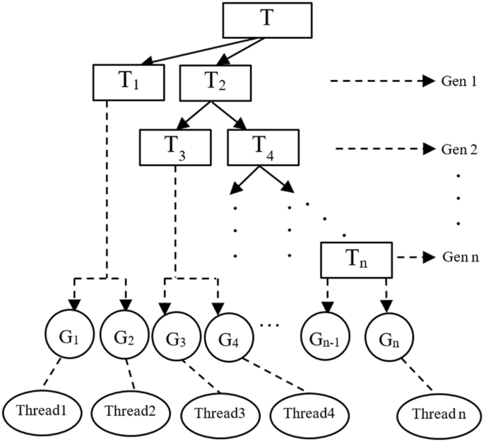
PMSA classification at thread-level

Prototypes generation starts with N random points in the normalized space. The \(N\) random points are antibodies. The training sample set T are antigens. Prototypes are constructed by using antibodies as the center. If the closest antigen belongs to class Cp to this center, this prototype covers class Cp. The radius is the distance between this center and the closest antigen of a different class \({\text{C}}_{\text{p}}^{'}\). In this case, the constructed prototypes of class Cp only covers training points of class Cp. However, some constructed prototypes are redundant since they cover the same training sample points. To remove the redundancy, the prototypes are evaluated for fitness.
Fitness calculation is measured using a metric called, Figure of Merit. Given a prototype G, the figure of merit \(F\) is defined as the number of points belongs to class \(C_{p}\) inside the prototype \(G\). Figure of merit represents the fitness of the prototype classifier. A large \(F\) is considered better in fitness than a smaller value of \(F\). Then all the \(F\) values of prototypes are calculated. The largest \(F\) is \(LF\). Only the prototypes with \(LF\) is used for this generation. Other prototypes are discarded. In order to find a prototype with a larger \(LF\), MSA starts a search in the neighborhood area using mutation.
Prototypes mutation starts after the \(LF\) of the prototypes for each class is calculated. The aim of mutation is to find a larger \(LF\). MSA starts a search by selecting one prototype each class to mutate to several prototypes. This selection is a stochastic method that randomly select one prototype within figure of merit distribution of the prototypes. This distribution can ensure that prototypes with larger figure merit will have higher probability during our selection. After this prototype is chosen, the center of this prototypes will mutate to \(N\) points. The mutations of the points follow a certain randomness to ensure that they are in the neighborhood areas. The mutation usually rans for several iterations. It stops when we could not find a larger \(LF\) for all classes or it reaches to certain number of iterations, which is set by user. Once the mutation stops, these mutated points are used as random points when it returns to step a) to generate new prototypes. Therefore, the artificial immune system approach is to continually develop new prototypes (antibodies) to cover as many as samples points (antigens).
-
2.
Partition process this process begins after mutation stops. The training sample points inside the prototypes with \(LF\) of each class is denoted as subset \(T_{1}\), which are considered training points that covered by optimal prototypes. These prototypes are optimal and strong classifiers which classify class points correctly. It is different from Boosting algorithm which combines weak classifiers [45]. The partition process removes \(T_{1}\) out from the original training set \(T\). Then the remaining sets will enter the evolution process to construct new prototypes again.
Compare to the training process for some machine learning algorithms, such as SVM, which uses the whole training set to seek hyperplane classifiers that has the largest margin, MSA gradually divides the training set into smaller subsets. MSA trains classifiers for those smaller problems with a margin preset by the user for error. The advantage of this decomposition is breaking the whole training sets into a number of small subsets makes it easier to find classifiers for non-separable cases. Specifically, given training set S, MSA generates a partition of the set \(T\) and each partition is denoted as subsets \(T_{1}\), \(T_{2}\), \(T_{3}\),….The training set can be viewed as a union of its subsets and the subsets are non-empty and non-overlapping. In particular, we formulate the partition process as below:
The above partition process is conducted at runtime. MSA iteratively seeks the prototypes for the subsets, and the partition subsets are generated sequentially. Next, those training points fall into the prototypes are removed from the whole training set, and the remaining training sets recursively perform the partition task until no training points left.
Ideally, MSA stops when all the points are partitioned out and the reduced set becomes empty However, considering the misclassified and unclassified points, the ideal case may not be reached. Therefore, some parameters values are preset to prevent the algorithm does not converge for a long time. First, the portion of the members in the reduced set drops to a user set small limit, e.g., 0.001%. Second, the number of generations raises to a user set limit, e.g., 20. As long as one of the above conditions meets, MSA stops the training process.
3.3 Parallel MSA
PMSA iteratively solve the problems and get the optimized classifier, i.e., prototypes. The prototype regions are the decision boundaries for classification. The classification process is proposed to implement it in parallel. The algorithms of PMSA is presented as follows:
Consider a multiclass (\({\text{P}}\) classes) problem. Each class can be denoted as class \({\text{C}}_{\text{p}} \left( {{\text{p}} = 1,2,..{\text{P}}} \right)\). There are \({\text{O}}\) objects in raw data belongs to \({\text{P}}\) classes. Each sample point is an n-dimensional feature vector x with m attributes, and it can be denoted as \({\text{x}}_{\text{i}} = \left( {x_{1} , \ldots ,x_{m} } \right)\). We present margin setting algorithm in five phases below: prototype generation, fitness calculation, prototype mutation, partition and parallel classification testing.
Algorithm 1 PMSA |
Notation: |
Unif (A): uniform distribution on set A. |
χ: margin |
\({\text{M}}:\) number of iterations during mutation |
\({\text{Q}}:\) number of partitions/generations |
MM: Maximum Mutation |
MQ: Maximum Generation |
N: Number of random points |
INPUT: |
1) Training set \(T = \left\{ {\left( {x_{1} , \ldots ,x_{m} } \right)} \right\}\), consists of m training samples. Each training sample \(x_{k} \left( {1 \le k \le m} \right)\) is n-dimension vector (\(n \ge 2)\) with class label \({\text{C}}_{p } \left( {p = 1, \ldots ,P} \right)\). (\(P > 1\)) classification problem, |
2) Testing set \(S = \left\{ {\left( {y_{1} , \ldots ,y_{n} } \right)} \right\}\)., consists of n unknown label testing samples. |
INITILIZE: |
Set MM \(\leftarrow\) 20; MG \(\leftarrow\) 20; N \(\leftarrow\) 20; M \(\leftarrow\) 0; N \(\leftarrow\) 0; |
REPEATE: |
1. Normalize \(T\) into [0, 1] space. Randomly select \({\text{N}}\) n-dimension points \(\upomega_{i} \left( {1 \le i \le N} \right) \in {\text{Unif }}\left[ {0,1} \right]\). |
REPEATE: |
Prototype Generation |
2. Build prototypes \(G_{i} = \left( {\omega_{i} ,R_{i} ,C_{p} } \right), 1 \le i \le N,p = 1, 2 , \ldots ,P\}\). Compute the centers \(\upomega_{i}\) of \(G_{i}\) of class \(C_{p}\) that has the minimum Euclidean distance from \(\omega_{i}\) to \(x_{k}\): |
\(d_{k} = \hbox{min} \left| {\left| {\upomega_{i} - x_{k} } \right|} \right|.\) (3) |
3. Compute the radius \(R_{k}\) of \(G_{i}\). It equals the minimum Euclidean distance from \(\omega_{i}\) to \(x_{j}\): |
\(R_{k} = min\omega_{i} - x_{j} , j \ne k\). (4) |
Fitness Calculation |
4. Compute the fitness, measured by figure of merit of the prototype. The figure of merit of prototype \({\text{G}}_{i}\) is denoted as \({\text{F}}_{{{\text{G}}_{\text{i}} }}\), i.e., the number of class \(C_{p}\) data samples inside of \({\text{G}}_{\text{i}}\) geometrically. Suppose class label \(C_{p}\) contains total h prototypes for during the current iteration. The largest figure of merit among all h prototypes is \(LF\): |
\(LF = { \hbox{max} }\left\{ {{\text{F}}_{{{\text{G}}_{1} }} ,{\text{F}}_{{{\text{G}}_{2} }} , \ldots ,{\text{F}}_{{{\text{G}}_{\text{h}} }} } \right\}\). (5) |
Prototypes Mutation |
5. Select one center \(\omega_{i}^{ '}\) of prototype \(G_{i}\) each class to mutate to N random points in the neighborhood area of \(\omega_{i}^{ '}\). Calculate the proportional of the prototypes of figure of merit \(f_{p}\): |
\(f_{p} = \frac{{F_{{G_{i} }} }}{{\mathop \sum \nolimits_{1}^{h} F_{{G_{i} }} }}\). (6) |
If i in \(\omega_{i}^{ '}\) satisfy the following distribution function and \(\upzeta \in {\text{Unif }}\left[ {0,1} \right]\): \(\mathop \sum \limits_{\xi = 1}^{i - 1} f_{\xi } <\upzeta \le \mathop \sum \limits_{\xi = 1}^{i} f_{\xi }\). Select \(\omega_{i}^{ '}\) to mutate to another N points. The mutated N points are: |
\(\omega_{i}^{'} + \varepsilon \alpha U\). (7) |
Where \(\varepsilon\) is random sign symbol {-1,1}. \(\alpha \in {\text{Unif }}\left[ {0,1} \right]\). U is the maximum perturbation: |
\(U = \left\{ {\begin{array}{*{20}c} {\omega_{i}^{ '} } & {if \omega_{k} \le \frac{{\hbox{min} \left\{ {x_{k} } \right\} + { \hbox{max} }\left\{ {x_{k} } \right\} }}{2}} \\ { { \hbox{max} }\left\{ {x_{k} } \right\} - \omega_{i}^{ '} } & {Otherwise} \\ \end{array} \left( {1 \le k \le m} \right)} \right.\). (8) |
6. \({\text{M}} \leftarrow {\text{M}} + 1\), enter the next mutation round. The largest figure of merit in current generation M + 1 is denoted as \({\text{LF}}^{M + 1}\), the previous generation is \({\text{LF}}^{M}\). |
UNTIL \(M > MW\) \(\parallel\) \(LF^{M} > LF^{M + 1}\) |
Partition |
7. Partition the training set \(T\) by removing all data in the prototype \(G_{i}^{o}\). \(G_{i}^{o}\) is the optimal prototyope with largest figure of merit \({\text{LF}}^{M}\), and radius \(R_{i,Q}\), where |
\(R_{i,Q} = \left( {1 - \chi } \right)R_{i,Q}\). (9) |
We tune the margin \(\chi (0 \le \chi < 1)\) to shrink the radius of hyperspheres. A larger margin tends to yield better generalization. The reduced training set is \({T^{\prime}}\). |
8. \(T \leftarrow T^{\prime}\), update the training set \(T\) as the content of reduced set \(T^{\prime}\). |
9. \(Q \leftarrow Q + 1\), enter the next generation round. |
UNTILE \(T^{\prime} = \emptyset \parallel\) \(Q > MQ\) |
Parallel Classification |
10. After partition completes and all the prototypes generated in all \({\text{Q}}\) generations for all classes \({\text{C}}_{\text{p}} \left( {{\text{p}} = 1,2, \ldots {\text{P}}} \right)\)., the prototypes for all p classes are |
\({\text{G}}^{{\prime }} = \mathop {\bigcup }\limits_{t = 1}^{\text{Q}} \mathop {\bigcup }\limits_{{C_{p} = 1}}^{P} G_{i}^{o} |_{{t,C_{p} }}\). (10) |
11. Dynamically assign n threads/processes for testing. Each thread/process handles one prototype \({\text{G}}^{{\prime }} .\) Each thread execute: For all points \(y_{i}\) in test set \(S\), we compute the Euclidean distance between \(y_{i}\) and \(\upomega_{i}\), where \(\upomega_{i}\) is all the centers of prototypes \({\text{G'}}\left( {\omega_{i} ,R_{i} ,C_{p} } \right),\), and if |
\(\left| {\left| {y_{i} -\upomega_{i} } \right|} \right| \le R_{k}\). (11) |
Set variable Output = 1. The points \(y_{i}\) belongs to class \(C_{p}\). \(y_{i} = C_{p}\). Otherwise, Output = 0. |
12. Gather results from all threads. Logic OR operators is performed on all output to detersmine the classification results. \(y_{i} = C_{p}\) when Output = 1. Otherwise, Output = 0. \(y_{i}\) is not classified. |
To aforementioned mathematical model of the parallel classification of MSA is presented in Fig. 2. Training process of MSA completes after several iterations/generations, denoted as Gen 1, Gen2,…, Gen n, which yields multiple prototypes \(G_{1}\) … \(G_{n}\) as its classification decision boundaries. For each generation, MSA splits the training set T into two subsets. One subset is the training points covered by the prototypes. The other subset is the remaining unclassified class points. MSA usually keeps only one prototype with \(LF\) for each class. If the training points of one class are all classified after several generations, no more prototypes will be generated for that class. However, MSA still continues to generate prototypes to cover the remaining unclassified training points. If there are P classes, the maximum number of prototypes can yield for one generation is P.
Take a look at a binary classification problem (class 1, 2) shown in Fig. 2. The training set T is split into subsets \(T_{1}\) and \(T_{2}\) in the first generation (Gen 1). Training set \(T_{1}\) is the class points containing class 1 points covered by G1 and class 2 points covered by \(G_{2}\). The remaining class points are the training set \(T_{2}\). In the next generation (Gen 2), \(T_{2}\) is split to \(T_{3}\) and \(T_{4}\). Training set \(T_{3}\) is the class points containing class 1 points covered by \(G_{3}\) and class 2 points covered by \(G_{4}\). Training set \(T_{4}\) contains the remaining unclassified points. Eventually, all class points are classified by prototypes {G1…Gn}. Note that each generation does not necessarily yield one prototype for each class. For example, during some generation, all class 1 points have been classified, the remaining set only contains class 2 points. In this case, the next generation will only yield one prototype for class 2. Therefore, MSA tends to classify the total class points using a disjunction of several prototypes generated through multiple generations.
In addition, it can be seen from Fig. 2, the proposed parallel classification is conducted at thread-level parallelism (TLP). TLP concentrates on splitting the tasks so that each subtask is concurrently running on the same data across different processing unit [46]. MSA classification tasks are conducted sequentially through a series of classifiers. We consider an efficient parallel practice is to split this whole sequential task into several subtasks. In MSA, it generates a sequence of prototypes {G1…Gn} as classifiers. Each classifier exhibits good generation with a low VC dimension. The unknown or new data can be classified by the prototypes {G1…Gn} in parallel for each class independently. Each classifier can be allocated a thread/process to test the unknown belongs to that class or not. If the classifier can classify the unknown correctly, output 1. Otherwise, output 0. Then the overall classification result is a simple logic OR of output from each thread. For example, it can be seen from Fig. 2, we allocate thread 1 to n to prototypes \(\{ G_{1} \ldots G_{n} \}\). For class 1, {G1, G3,…} are the classifiers that use thread 1, 3,…to test the unknown data can be classified and recognized as class1 independently. For class 2, {G2, G4,…} are the classifiers that use thread 2, 4, …to test the unknown data can be classified and recognized as class2 independently.
4 Experiments and results
To test the efficiency of the proposed PMSA, our experiment was conducted in two stages. First, we open a pool of workers for MSA classification applied to image segmentation. Second, threads are used to spawn a number of threads during runtime and speed up the MSA classification. Several machine learning benchmark data sets are chosen for the classification tasks. Our parallel experiments are all conducted on a machine with Intel Xeon processor E5520, 2.27 GHz. It is equipped with 2-processors, and each processor has 4 cores. Each core uses hyper-threading. Totally we can utilize 16 logic processors to accelerate the performance of MSA classification in the testing phase.
4.1 Image segmentation
MSA is a supervised learning algorithm that was applied to discriminate the objects in images. The intensity of the color pixels is chosen as the features for classification. Two benchmark color images: Airplane and Peppers are used in the experiment as shown in Fig. 3a and b. The image sizes of Airplane is 321 × 481 pixels and Peppers is 512 × 512 pixels in R, G, B components respectively. The image segmentation tasks are as follows: MSA performs segmentation on the airplane from its background as shown in Fig. 3c. To implement it, we consider airplane and background are two classes. Training sets are constructed by randomly selecting 20 points from airplane and another 20 points from the pixels are not airplane. After MSA training, the generated prototypes are used to perform a binary classification on the image Airplane. For image Peppers, MSA remove the red peppers out from the image as shown in Fig. 3d. To perform MSA classification, red peppers is one class. Other peppers, including dark green and light green peppers, is another class. Training sets are 20 random points from each class, i.e., total 40 points. Overall, it can be seen that MSA yields good performance for image segmentation. We also compare the results with SVM and ANN.

PMSA for image segmentation. a Image “Airplane”; b Image “Peppers”; c classification results for Image “Airplane”; d classification results for Image “Peppers”
To accelerate the MSA classifications on the image data sets, we utilized the parallel pool. It opens a set of workers that uses parallel pool to execute the statements in parallel as shown in Fig. 4. The number of workers corresponds to the number of processes that can be run simultaneously. To test the effectiveness of the parallel workers on multicore and multiprocessor system, we choose different size of the data sets. For simplicity, we resize the Airplane image by factor of 2, 3, 4…10, and perform the image segmentation tasks. The number of image pixels are the total of the data points during MSA classification. Each data has three features, i.e., the intensity value in R, G, B channels respectively. The execution time of non-parallel, 2, 4, 6 8, 12 and 16 workers are reported in Table 1. Serial MSA execution time is when we run it on the single processor system sequentially without any parallel scheme. It shows that the execution time is greatly reduced when the number of workers increases. Specifically, the execution time for 8 workers is reduced more than 6, 4 and 2 workers. For example, when the image size is 3210 × 4810, the execution time for segmenting the airplane out from its background is reduced from 280.002 s for the non-parallel scenario to 58.724 s for 8 workers, and only 38.419 s for 16 workers.

PMSA using parallel pool of workers
Next, we investigate the speedup ratio and parallel efficiency obtained by the parallel pool. The speedup ratio R is the relative performance measurement between a single processor system and a multiprocessor system. It is calculated as follows:
where \(T_{s}\) is the execution time on a single processor system, \(T_{m}\) is the execution time on a multiprocessor system with m processors. The parallel efficiency E can be estimated as the ratio of speedup to the number of processors. It measures the fraction of time for which a processor is being used on the computation. Efficiency is calculated as:
The speedup ratio is reported in Table 2 and Fig. 5. It shows that the speedup increases when we increase the number of workers. The speedup has a higher value for 16 workers than 12, 8, 4 and 2 workers for all image sizes. The average speedup ratio is 7.06 for 16 workers, and 4.54 for 8 workers, comparing to 1.93 for 2 workers. We also note that the primary increase of speedup ratio happens before the image size increases to a certain amount. For example, the speedup ratio increases from 3.11 to 4.26 after the image sizes rise up to \(0.4 \times 10^{7}\) image pixels for 6 workers. After that, the speedup ratio increases slowly, only to 4.31 when the number of image pixels reach to \(4.6 \times 10^{7}\). Similarly for 16 worker case, the speedup ratio rises up quickly from 5.93 to 7.22 when we enlarge the image size to 963 × 1443 pixels in its R, G, B channel. After that, there is only an 0.06 speedup ratio gain after the image resizes to 3210 × 4810 pixels.

Speedup ratio of PMSA for image segmentation
The parallel efficiency E of different workers is presented in Fig. 6. It is expected that the E reaches to 1 if the parallel algorithm scales linearly and achieves very good performance. When PMSA is tested with 2 workers, E reaches to 1 when the image contains \(1.1 \times 10^{7}\) pixels. However, E drops to when the number of workers increases. Specifically, the average value of E falls to 0.81 for 4 workers, 0.68 for 6 workers, 0.56 for 8 workers, 0.49 for 12 workers and 0.44 for 16 workers. This comes from the fact that PMSA employs a thread-level data parallelism which distributes the generated prototypes across different workers. It is less efficient than a task-parallelism.

Parallel efficiency of PMSA for image segmentation
4.2 Benchmark datasets
We also implement PMSA classification using Threads. For multicore and multiprocessor system, each independent processor owns a specific amount of physical resources. In order to take full advantage of the thread-level parallelism, a practical way is to set the proper number of threads equaling to the number of prototypes generated. To test the PMSA performances, several machine learning benchmark datasets from the UCI machine learning repository are chosen for the experiment [47]. The details of the datasets are shown in Table 3 below. There are five datasets: Pima Indians Diabetes, Wisconsin Breast Cancer, Australian Credit Approval, Wine and Svmguide2. One-third of the datasets are randomly chosen for training, and the remaining data for testing. We repeat the experiments for ten times and compute the average results.
To validate the classification performance, we compared the PMSA to another two other state-of-the-art algorithms, SVM and ANN. There are two considerations. First, both PMSA and SVM are margin-based classifiers. Their performances are affected by margin, which is the distance from each example to the decision boundary. Second, both SVM and ANN are popular supervised classification algorithms that were applied to test UCI benchmark datasets. The default parameters are chosen for MSA. We set the margin χ of MSA from 0 to 0.5 for classification results. The SVM default parameters we chose are Radius basis function (RBF) kernel, with regularization parameter C = 1. The kernel parameter γ is set as the reciprocal of the number of features in the datasets. ANN implements a two-layer feed-forward backpropagation neural network with 10 neurons in its hidden layers. The classification performance of PMSA is reported in Table 4. It can be seen that PMSA yields better performance than SVM and ANN for all datasets.
The execution time and speedup of PMSA are reported in Table 4. This approach generated the number of threads that equals to the number of prototypes. Therefore, the number of threads are dynamically determined after the training process of MSA. This thread-level parallelism achieves the best speedup ratio 65.69 for Indian Diabetes dataset. When a large number of prototypes are generated, the speedup capacity will be affected. In this case, the communication overhead increases when splitting the classification task to a large number of threads. Our algorithm overall shows good speedup results.
5 Conclusion
In this work, we proposed a novel parallel implementation of a supervised learning algorithm, called margin setting algorithm. It is the first work to design a parallel mechanism to speed up the classification phase of the MSA. Our proposed parallel mechanism includes using parallel pool of workers with the specified number of workers to run MSA classification in parallel. In addition, threads are implemented to dynamically spawn the number of threads in runtime, and they spread the classification work among multi-core and multiprocessor system. Extensive experiments have been conducted to analyze the execution time and speedup of the PMSA. We applied PMSA on image data to perform image segmentation, and then classification on benchmark data sets from the UCI machine learning repository. We vary the number of workers during parallel implementation on image segmentation. The results show that speedup ratio tends to be higher when the image increase to a certain size. To validate the correctness of the proposed algorithm, the classification performance is also compared with SVM and ANN for benchmark data. The experimental results show that the proposed PMSA yields good classification accuracy and greatly reduces the computation time during testing phase. In the future, we will work on parallel mechanism on the training process of PMSA. Larger scale datasets will be used to test the robustness of the proposed parallel learning algorithm. One limitation of this work is that the thread-level parallelism that PMSA employs only relies on multicore and multiprocessor system. We will deploy PMSA on GPU and compare it with other deep learning algorithms, such as convolutional neural networks and recurrent neural networks, for data-intensive applications.
References
Jordan MI, Mitchell TMJS (2015) Machine learning: trends, perspectives, and prospects. Science 349(6245):255–260
Gupta P, Sharma A, Jindal RJWIRDM, Discovery K (2016) Scalable machine-learning algorithms for big data analytics: a comprehensive review. Data Min Knowl Discov 6(6):194–214
Sanchez V, Pfeiffer C, Skeie N-O, Networks A (2017) A review of smart house analysis methods for assisting older people living alone. J Sens Actuat Netw 6(3):11
Dahmen J, Thomas BL, Cook DJ, Wang XJS (2017) Activity learning as a foundation for security monitoring in smart homes. Sensors 17(4):737
Liu Y, Bi J-W, Fan Z-P (2017) Multi-class sentiment classification: the experimental comparisons of feature selection and machine learning algorithms. Exp Syst Appl 80:323–339
Arulmurugan R, Sabarmathi K, Anandakumar H (2017) Classification of sentence level sentiment analysis using cloud machine learning techniques. Cluster Comput 22(Suppl 1):1199–1209
Xu H, Gao Y, Yu F, Darrell T (2017) End-to-end learning of driving models from large-scale video datasets. In: IEEE conference on computer vision and pattern recognition (CVPR), IEEE, pp 3530–3538
Latif A, Rasheed A, Sajid U, Ahmed J, Ali N, Ratyal NI, Zafar B, Dar SH, Sajid M, Khalil T (2019) Content-based image retrieval and feature extraction: a comprehensive review. Math Probl Eng. https://doi.org/10.1155/2019/9658350
Nobile MS, Cazzaniga P, Tangherloni A, Besozzi D (2016) Graphics processing units in bioinformatics, computational biology and systems biology. Brief Bioinf 18(5):870–885
Cuomo S, De Michele P, Di Nardo E, Marcellino L (2018) Parallel implementation of a machine learning algorithm on GPU. Int J Parallel Program 46(5):923–942
Tan K, Zhang J, Du Q, Wang X (2015) GPU parallel implementation of support vector machines for hyperspectral image classification. IEEE J Select Top Appl Earth Observ Remote Sens 8(10):4647–4656
Liu Y, Yang J, Huang Y, Xu L, Li S, Qi M (2015) MapReduce based parallel neural networks in enabling large scale machine learning. Comput Intell Neurosci. https://doi.org/10.1155/2015/297672
Low Y, Gonzalez J, Kyrola A, Bickson D, Guestrin C, Hellerstein J (2010) GraphLab: a new framework for parallel machine learning. In: Proceedings of the twenty-sixth conference on uncertainty in artificial intelligence, 2010. AUAI Press, pp 340–349
Diaz J, Munoz-Caro C, Nino A (2012) A survey of parallel programming models and tools in the multi and many-core era. IEEE Trans Parallel Distrib Syst 23(8):1369–1386
Lotrič U, Dobnikar A (2005) Parallel implementations of feed-forward neural network using MPI and C# on. NET platform. In: Ribeiro B, Albrecht RF, Dobnikar A, Pearson DW, Steele NC (eds) Adaptive and natural computing algorithms. Springer, Berlin, pp 534–537
Zhao H-X, Magoules F (2011) Parallel support vector machines on multi-core and multiprocessor systems. In: 11th international conference on artificial intelligence and applications (AIA 2011), IASTED
Caulfield HJ, Karavolos A, Ludman JEJIS (2004) Improving optical Fourier pattern recognition by accommodating the missing information. Inf Sci 162(1):35–52
Fu J, Caulfield HJ, Wu D, Tadesse W (2010) Hyperspectral image analysis using artificial color. J Appl Remove Sens 4(1):043514
Wang Y, Fu J, Adhami R, Dihn HJTISJ (2016) A novel learning-based switching median filter for suppression of impulse noise in highly corrupted colour images. Imaging Sci J 64(1):15–25
Wang Y, Adhami R, Fu J (2015) A new machine learning algorithm for removal of salt and pepper noise. In: Seventh international conference on digital image processing (ICDIP 2015), 2015. International Society for Optics and Photonics, p 96311R
Wang Y, Adhmai R, Fu J, Al-Ghaib H (2015) A novel supervised learning algorithm for salt-and-pepper noise detection. Int J Mach Learn Cybern 6(4):687–697
Wang Y, Amin MM, Fu J, Moussa HBJIA (2017) A novel data analytical approach for false data injection cyber-physical attack mitigation in smart grids. IEEE Access 5:26022–26033
Igwe OM, Wang Y, Giakos GC (2018) Activity learning and recognition using margin setting algorithm in smart homes. In: 2018 IEEE ubiquitous computing, electronics and mobile communication conference (UEMCON), New York, Nov 8–10, 2018. IEEE, pp 294–299
Amado N, Gama J, Silva F (2001) Parallel implementation of decision tree learning algorithms. In: Portuguese conference on artificial intelligence. Springer, Berlin, pp 6–13
Ben-Haim Y, Tom-Tov E (2010) A streaming parallel decision tree algorithm. J Mach Learn Res 11:849–872
Lukač N, Žalik B (2015) Fast approximate k-nearest neighbours search using GPGPU. In: Cai Y, See S (eds) GPU computing and applications. Springer, Berlin, pp 221–234
Li S, Amenta N (2015) Brute-force k-nearest neighbors search on the GPU. In: International conference on similarity search and applications. Springer, Berlin, pp 259–270
Andrade G, Viegas F, Ramos GS, Almeida J, Rocha L, Gonçalves M, Ferreira R (2013) GPU-NB: a fast CUDA-based implementation of naive bayes. In: 2013 25th international symposium on computer architecture and high performance computing. IEEE, pp 168–175
Zhou L, Yu Z, Lin J, Zhu S, Shi W, Zhou H, Song K, Zeng X (2014) Acceleration of Naive–Bayes algorithm on multicore processor for massive text classification. In: 14th international symposium on integrated circuits (ISIC). IEEE, pp 344-347
Ali N, Bajwa KB, Sablatnig R, Chatzichristofis SA, Iqbal Z, Rashid M, Habib HA (2016) A novel image retrieval based on visual words integration of SIFT and SURF. PLoS ONE 11(6):e0157428
Bagchi P, Bhattacharjee D, Nasipuri MJMT (2016) A robust analysis, detection and recognition of facial features in 2.5 D images. Multimed Tools Appl 75(18):11059–11096
Ratyal NI, Taj IA, Sajid M, Ali N, Mahmood A, Razzaq S (2019) Three-dimensional face recognition using variance-based registration and subject-specific descriptors. Int J Adv Robot Syst 16(3):1729881419851716
Ali N, Zafar B, Iqbal MK, Sajid M, Younis MY, Dar SH, Mahmood MT, Lee IH (2019) Modeling global geometric spatial information for rotation invariant classification of satellite images. PLoS ONE 14(7):e0219833
Lin T-K, Chien S-Y Support vector machines on gpu with sparse matrix format. In: Ninth international conference on machine learning and applications (ICMLA), 2010. IEEE, pp 313–318
Chang EY (2011) Psvm: Parallelizing support vector machines on distributed computers. In: Chang EY (ed) Foundations of large-scale multimedia information management and retrieval. Springer, Berlin, pp 213–230
You Y, Song SL, Fu H, Marquez A, Dehnavi MM, Barker K, Cameron KW, Randles AP, Yang G Mic-svm: Designing a highly efficient support vector machine for advanced modern multi-core and many-core architectures. In: 28th International parallel and distributed processing symposium. IEEE, pp 809–818
Li W, Fu H, You Y, Yu L, Fang J (2017) Parallel multiclass support vector machine for remote sensing data classification on multicore and many-core architectures. IEEE J Select Top Appl Earth Observ Remote Sens 10(10):4387–4398
Dahl G, McAvinney A, Newhall T Parallelizing neural network training for cluster systems. In: Proceedings of the IASTED international conference on parallel and distributed computing and networks, 2008. ACTA Press, Calgary, pp 220–225
Huqqani AA, Schikuta E, Ye S, Chen P (2013) Multicore and gpu parallelization of neural networks for face recognition. Procedia Comput Sci 18:349–358
Ratyal N, Taj IA, Sajid M, Mahmood A, Razzaq S, Dar SH, Ali N, Usman M, Baig MJA, Mussadiq U (2019) Deeply learned pose invariant image analysis with applications in 3D face recognition. Math Probl Eng. https://doi.org/10.1155/2019/3547416
Sajid M, Ali N, Dar SH, Iqbal Ratyal N, Butt AR, Zafar B, Shafique T, Baig MJA, Riaz I, Baig S (2018) Data augmentation-assisted makeup-invariant face recognition. Math Probl Eng. https://doi.org/10.1155/2018/2850632
Sajid M, Iqbal Ratyal N, Ali N, Zafar B, Dar SH, Mahmood MT, Joo YB (2019) The impact of asymmetric left and asymmetric right face images on accurate age estimation
Chetlur S, Woolley C, Vandermersch P, Cohen J, Tran J, Catanzaro B, Shelhamer E (2014) cudnn: efficient primitives for deep learning. arXiv preprint arXiv:1410.0759
Ma X, Dai Z, He Z, Ma J, Wang Y, Wang YJS (2017) Learning traffic as images: a deep convolutional neural network for large-scale transportation network speed prediction. Sensors 17(4):818
Freund Y, Iyer R, Schapire RE, Singer Y (2003) An efficient boosting algorithm for combining preferences. J Mach Learn Res 4:933–969
Cheng Z, Schmidt T, Liu G, Doomer R (2017) Thread-and data-level parallel simulation in SystemC, a Bitcoin miner case study. In: IEEE international high level design validation and test workshop (HLDVT), IEEE, pp 74–81
Frank A, Asuncion A (2010) UCI machine learning repository. University of California, Irvine, CA, School of information and computer science. http://archive.ics.uci.edu/ml. Accessed June 2018
Acknowledgements
This work is partially supported by Defense Intelligence Agency (DIA) under award HHM402-18-FOA-399-A.
Author information
Authors and Affiliations
Corresponding author
Ethics declarations
Conflict of interest
The authors declare that they have no conflict of interest.
Additional information
Publisher's Note
Springer Nature remains neutral with regard to jurisdictional claims in published maps and institutional affiliations.
Rights and permissions
About this article

Cite this article
Wang, Y., Fu, J. & Wei, B. A novel parallel learning algorithm for pattern classification. SN Appl. Sci. 1, 1647 (2019). https://doi.org/10.1007/s42452-019-1687-6
Received:
Accepted:
Published:
DOI: https://doi.org/10.1007/s42452-019-1687-6