Performance improvement of intrusion detection system using neural networks and particle swarm optimization algorithms

Abstract

Intrusion detection system is considered as a decision-making tool in the networks. Mainly, an intrusion is an attempt to violate the security mechanisms and its rules. The aim of an intrusion detection system is to monitor network traffic and explore unusual behavior that may be an attack. If a package has a different pattern toward its standard behavior, it can be categorized as abnormal conditions and consequently an attack or intrusion. In this paper, a pre-processing is performed on KDD-CUP99, NSL-KDD and CIDD dataset to choose a subset of the features, reduce dimension and then normalize data. Combination of particle swarm optimization and neural network algorithms are used to recognize intrusions which can efficiently classify the attacks and reduce the number of false alarms and improve detection rates. Obtained results show that proposed method provides a higher accuracy and performance comparing with other algorithms to detect different classes of attacks.

1 Introduction

It is with the purpose of violating security policies such as confidentiality, integrity and accessibility that one tries to intrude on a network [1]. Some considerable researches have been conducted on detection and prevention of intrusion in the field of information security. Intrusion detection can be a classification system of the network traffic which determines whether the received packet is normal or not [2]. Denning is the first person who studied intrusion-detection systems [3]. From then, numerous methods have been invented onwards to improve the function of intrusion detection systems including statistical, machine learning and data mining methods. A good intrusion-detection system must have minimum false negative rate and a high detection rate [4]. One thing that is quite significant in computer systems is intrusion detection. An intrusion detection system is a software or hardware which monitors the computer network to see if there is any harmful activity or any violation of the management and security policies and then it reports to the network management sector. Intrusion-detection systems must detect and recognize any kind of unpermitted usage of the system, or any kind of abuse or activity by both internal and external users that would harm the computer. Usually, intrusion-detection systems are used along with firewalls and act as a complementary security-wise for them. Traditional intrusion-detection system cannot adapt to new intrusions; thus, nowadays intrusion-detection is mainly based on data mining and meta-heuristic algorithms. One area in which intrusion-detection can be helpful is finding new attacks. Rule-based intrusion detection systems such as snort cannot recognize the attacks correctly in most cases and have a high error rate. In particular, these systems are not intelligent and the user is getting involved in rule and policy making. This type of systems is called signature-based system or abuse-based system [5]. However; anomaly-based methods are the opponents of the signature-based methods which are able to detect new attacks. Of course, in some cases they have some false alarms [6]. Numerous methods have been presented to solve intrusion-detection problems, each of which has its own specific rate of precision in detecting attacks. In this article, it has been aimed to signify proposed algorithm’s ability to detect and reduce the likelihood of mistakes being made by using Neural Networks (NN) integrating with Particle Swarm Optimization (PSO) algorithm. Intelligence of this algorithm rise exponentially which leads to reduce the work that network managers have to be done. In the first section, literature of the previously conducted researches has been studied and discussed in brief. The second section is associated with the tools and its mechanism is explained. In the third section, the proposed system and its function has been expressed. The fourth section depicts how the experiments are done and the other methods are compared with one another in this section. Final section provides information regarding the results obtained by the algorithm.

2 Previous works

Singh et al. proposed an Online Sequential Extreme Learning Machine (OS-ELM) based method for intrusion detection. Their proposed method uses alpha profiling to reduce the time complexity while irrelevant features are discarded using consistency and correlation which reduce state space. Instead of sampling and beta profiling was used to reduce the size of the training dataset. The standard NSL-KDD dataset is used for performance evaluation of the proposed method. In this paper, space and time complexity was discussed that showed an improvement comparing with the other methods. The experimental results yielded an accuracy rate of 98.66%, error rate of 1.74% and detection time of 2.43 s [8].

In 2015, Chattopadhyay overviewed the neural network’s applications in IDSs and shed light to a positive process of the neural network is being used to detect intrusions. In addition, a multi layered perceptron (MLP) Neural Network based structure was presented by them in order to develop substantially application in KDD99. According to the identified patterns of the structure of the detected attacks in the database, the proposed MLP algorithm had better outcomes by using back-propagation in comparison with the recurrent neutral networks and analysis of the main components based on mutual actions. A detection rate of more than 99.10% was reported for the presented neural network. Therefore, the presented information depicts how the MLP method have the more efficient detection rate and how it can increase the system’s efficiency by reducing the cost of calculations without losing detection efficiency [9].

In 2015, Raman Singh, et al. wrote an article and offered a method based on online sequential extreme learning method (OS-ELM) for intrusion detection. Their suggested method uses alpha profile to decrease the computational time in such a way that irrelevant features are deleted by using correlations and agreements and that is how the working space is also reduced. In order to make the training dataset smaller, beta profile has been used instead of a sampling method. The security laboratory-knowledge discovery and data mining (NSL-KDD) has been used for the presented method to be evaluated. In this article, time and space complexities have been discussed and according to our investigation, this method has improved in comparison with the other methods. The experimental results depict a precision rate of 98.66% and an error rate of 1.74% as well as a 2.43-s detection time [8].

Again in 2015, Dash used two methods for training the neural networks. One of the methods uses Gravitational Search method and the other one use PSO algorithm combined with Gravitational Search method. These methods have been compared by Tirtharaj Dash in terms of how functional they are in training of the neural network with other optimization algorithms such as PSO, Gradient Descent algorithm, Genetic and also decision tree classification algorithm. Experiments are performed on NSL-KDD database and the results indicate an improvement in comparison with other methods. According to the results of the experiment, a precision rate of 94.90% was obtained for the method based on the gravitational search and for the network training; a precision rate of 98.13% was obtained based on PSO and gravitational search. It is also claimed that the suggested method is more suitable for imbalanced datasets [10].

In 2016, Chunlin Lu used a method based on backward neural network integrated with the Dempster-Shafer theory and Genetic Algorithm. In Dempster’s opinion, this method accelerates the process of attack detection and decreases false alarms and makes the system more stable. In brief, the process of this method is as follows: at first, the extracted features are divided into various subclasses. Then, according to these various subclasses and various models, the neural networks are trained to build a detection method. Ultimately, the Dempster-Shafer theory is used to integrate these results and obtain the ultimate ones. This method has been evaluated on KDD99 database. The results have shown that it will work well while the system is faced with different types of attacks and it has a maximum precision rate of 97.5 [11].

In 2016, Mehmod et al. used Ant Colony Optimization and selected optimal features and classified these features using Support Vector Machine (SVM). The outcome of this feature selection method is being used in KDD cup database and shows that SVM classifier has better results and a precision rate of 98.29% [12]. Sharma et al. employed artificial bee colony that is a team approach to detect and fight back DOS attacks in cloud environment. In this research, data was recalled from the network traffic, and after the bees were released, they were used to train the classifier and to test. After wards, attack is detected. Apparently, detection rate of artificial bee colony was higher than QPSO. An attack detection rate of 72.4% was obtained for this method [13]. Scott E. Coull et al. discusses the use of a specially tuned sequence alignment algorithm, typically used in bioinformatics to detect instances of masquerading in sequences of computer audit data. By using the alignment algorithm to align sequences of monitored audit data with known sequences to be produce by the user, the alignment algorithm can discover areas of similarity and derive a metric that indicates the presence or absence of masquerade attacks. Additionally, they present several scoring methods for accommodating variations in user behavior, and heuristics for decreasing the computational requirements of the algorithm [14].

3 MLP neural networks

Neural networks with two layers cannot implement nonlinear functions like XOR. But networks with more than two layers e. x. MLP Neural Network can solve this problem. These networks are able to present a nonlinear mapping with an arbitrary precision and they do that by selecting the number of neural cells and layers. It might be necessary to note that this number is not a large one in most cases. MLP neural network is a feed-forward neural network [15].

Each network has an input layer, a hidden one and an output layer and the cells of each layer are specified using the trial and error method. In the MLP networks, each neuron at any layer is connected to all of the neurons of the previous layers and such layers are called fully connected networks. The input layer is a transmitter and a means to provide data. The final layer or the output layer contains the values predicted by the network and it introduces the output of the model. The middle or hidden layers are transmitters and processor and this is where data are processed. In the MLP networks, there can be any number of hidden layers in the network. It is important to note that only one hidden layer can be enough in most cases. In some cases, the learning is facilitated when there are two layers. If there is more than one layer, the learning algorithms must be extended to all layers. There is no practical method to estimate the number of units (neurons) in the hidden layer. For this purpose, the trial and error must be used in order to obtain a desirable total mean error.

4 Neural network mechanism

In this stage, training set is used to create the initial structure of the neural network. In the suggested model, MLP Neural Network is used as the basic network. Necessary step is explained respectively as follows:

4.1 Generation of neural network initial structure

In this article, neural networks have 12 inputs. In the hidden layer, the number of neurons varies depending on the inputs, the number of samples and volume of input data. In the results section, the number of neurons used for each sample is specified. However, in order to make it simpler, 4 neurons are used in the hidden layer. Here, the number of classes is the same as outputs and since there are two normal and abnormal classes, there should be one neuron in the output layer. The structure of neuron in a neural network is displayed in Fig. 1 and the structure of used neural network is displayed in Fig. 2.

Fig. 1

Structure of a neuron

Fig. 2

Structure of used neural network

As it is seen in Fig. 1, a neuron contains a collector and an activator function. Here, tan-sigmoid activation function is used. Each neuron has a number of inputs and each input has some weights. The values of these inputs are multiplied by the weights and their sum is calculated at the end and the activator function provides the output. This process has been shown in formula (1) and the activator function has been shown in Eq. (2).

$${{\text{O}}_{\text{i}}} = {{\text{g}}_{\text{i}}} \left( {\mathop \sum \limits_{{{\text{i}}} = 1}^{{\text{n}}} \,{{\text{x}}_{\text{i}}} {{\text{w}}_{\text{i}}} + {{\text{b}}_{\text{i}}} } \right),$$

(1)

$${\text{g}}_{\text{i}} \left( {\text{x}} \right) = \tanh \left( {\text{x}} \right) = \frac{{{\text{e}}^{\text{x}} - {\text{e}}^{{ - {\text{x}}}} }}{{{\text{e}}^{\text{x}} - {\text{e}}^{{ - {\text{x}}}} }}.$$

(2)

As it is seen in the formula (1), ${\text{O}}_{\text{i}}$ is the output of a neuron, ${\text{g}}_{\text{i}}$ is the activator function, ${\text{x}}_{\text{i}}$ is the neuron input, ${\text{w}}_{\text{i}}$ is the weight of each inputs and ${\text{b}}_{\text{i}}$ is the bias constant. All of these factors make the output more precise. Adding bias facilitates the usage of the perceptron network. In the activator function, x is the input of the activator function and its output is hyperbolic tangent of x. Figure 2 displays the structure of used neural network. This neural network has 12 inputs, 12 neurons in layer 1 and 3 neurons in the layer 2. These two layers are components of the hidden layer and the output layer has one neuron since it has two components.

5 Particle swarm optimization algorithm (PSO)

This algorithm has been inspired by the movement of birds to find space and food. In this mode, birds like to fly and move in groups. In addition, if a bird spots food somewhere, it will move towards it. Therefore, both a personal and a group experience have been the inspiration of this method.

In this method, each particle remembers the situation with the best outcome at each stage. The best outcome is the best individual situation of each particle. These informational particles exchange information with each other no matter where they are and the search space for each particle is d.

• The movement of the particle depends on three factors.

• Current situation of the particle.

• The best situation the particle has experienced yet (Pbest).

• The best situation the entire series of particles have experienced yet (Gbest).

• Simulation operation is done as it has been displayed in Fig. 3.

  Fig. 3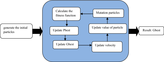

  

  Steps of PSO algorithm

New situation of each particle is obtained as follows:

$${\text{Present}}\left( {{\text{t}} + 1} \right) \, = {\text{ Present}}\left( {\text{t}} \right) + {\text{V}}\left( {{\text{t}} + 1} \right),$$

(3)

$${\text{V}}\left( {{\text{t}} + 1} \right) = {\text{V}}\left( {\text{t}} \right) \times {\text{W}} + {\text{C1}} \times {\text{Rand }}\left( {0, 1} \right) \times \left[ {{\text{Pbest}}\left( {\text{t}} \right) - {\text{Present}}\left( {\text{t}} \right)} \right] + {\text{C2}} \times {\text{Rand}}\left( {0, 1} \right) \times \left[ {{\text{Gbest}}\left( {\text{t}} \right) - {\text{Present}}\left( {\text{t}} \right)} \right].$$

(4)

In the Eq. (1), Present (t + 1) calculates the next situation of the particle, Present (t) specifies the current situation of the particle. V(t + 1) is called the velocity function which specifies the direction of the movement of particle which is calculated using Eq. (2). The Rand function generates the random numbers in the specified interval. C1 and C2 are the effect constants, Present (t) is the situation of each particle in the moment (t) and V(t) is the rate of location change or the velocity of the particle. C1 is a coefficient associated with the best situation of each particle and C2 is the coefficient associated with the best situation of neighborhoods and it helps change the velocity of the particle. These coefficients are usually equal to 2. W is the coefficient to change the previous velocity of particles. It is velocity of the particle movement towards the previous direction. The larger w is, the more general the search will be. In fact, as long as we have random initial velocity, it will be led towards the basic minimum [16]. The above formula (3, 4) causes that The particle moves toward the optimal solution(Gbest). Each particle conforms to these formulas (3, 4), Find the optimal answer(Gbest). Figure 4 shows the initial position of the particle and moves it according to formulas 3 and 4.

Fig. 4

Steps of PSO algorithm

The pseudocode of this algorithm is as shown in Fig. 5.

Fig. 5

Particle swarm optimization Pseudocode

6 Proposed method

Proposed algorithm is displayed in Figs. 6 and 7 and contains different parts which are related to one another to increase efficiency, precision and detection rates. We explain each part in separate sections. However, to put it briefly, in this structure first the transmitted packets are recorded by a node in a network and are saved in a database. In the following section, feature selection methods are explained to select proper features for intrusion detection. This section facilitates the classification for the training process. In the next step, selected data must be converted to numbers which can be detected by the neural network. In the following section, data is normalized between 0 and 1. Then, some of this normal data are used for training the neural network and some are used for testing the neural network. This data is selected randomly. The number of data varies to train and test and depends on the rate of precision as they vary in the experiments. In the next step, the optimal weights are pulled out through PSO algorithm and train the neural network by training data and obtained optimal weights. When the algorithm is applied as many times as determined in the beginning (converging condition), classification step is started. Data is divided into two classes: normal and abnormal. If data is indicated an anomaly or an intrusion, put in class 2 and otherwise, put in class 1. We can consider different classes depending on the type of application. Different types of attacks are examined in the experimental section in which various experiments have been discussed. At the end, in case there is an intrusion, the network manager or user will be given a proper signal or alarm.

Fig. 6

Preprocessing operations on data

Fig. 7

The proposed model for step 6.6–6.8

6.1 Datasets

In this article, KDDcup99 and NSL-KDD datasets have been used. KDDcup99 is used to train and test the system because it has useful features to detect the selected behaviors in the feature selection section. This database has 37 types of attack and 41 features. In the following section the ones being used is separated [17]. NSL-KDD database is the improved version of KDDcup99 in which the repetitive samples are eliminated and some new attacks are defined and is used for new studies. In this article, NSL-KDD database version 2015 and KDD-CUP99 database have been used [18]. Current dataset cannot be used due to the heterogeneity of user requirements and the distinct operating systems installed in the VMs, and the data size of Cloud systems. This paper presents a Cloud Intrusion Detection Dataset (CIDD)that is the first one for cloud systems and that consists of both knowledge and behavior based audit data collected from both UNIX and Windows users. With respect to current datasets, CIDD has real instances of host and network based attacks and masquerades, and provides complete diverse audit parameters to build efficient detection techniques [19].

6.2 Feature selection

Feature selection method is the process of detecting irrelevant and redundant information and eliminates them as much as possible. It is the process of dimensional reduction which allows the learning algorithms to act faster and more efficient. Therefore, classification can be improved. In this article, a filter is used based on Kolmogorov–Smirnov correlation to select a subclass of features that are useful in intrusion detection. According to this method, features that have a strong correlation with the class and don’t have a correlation with one another are the best features. In this method, a reformed Kolmogorov–Smirnov correlation-based fast redundancy removal filter (KS-CBF) has been used to select the features by class information label while it compares two features. 12 features are selected which are the most proper features for intrusion detection [20, 21].

These features are listed in the following:

• Service: network services at the target.

• SRC_bytes: the number of bytes of data moved from source to target.

• Dst_bytes: the number of bytes moved from target to source.

• Logged_in: if they successfully log in, the value 1 is given to them and otherwise, they are given 0.

• Count: the number of all communications with the same host as the connection present in the past two sections.

• Srv_count: the number of connections to similar services as the link that exists in the past two seconds.

• Serror_rate: the percentage of connections with the “SYN” error.

• Srv_rerror_rate: the percentage of connections with the “REG” error.

• Srv_diff_host_rate: percentage of connections to similar hosts.

• Dst_host_count: the number of connections to similar hosts.

• Dst_host_srv_count: a series of connections to the similar target port.

• Dst_host_diff_srv_rate: the percentage of connections in various services, among the connections collected in Dst_host_count.

6.3 Data preprocessing

Preprocessing includes two operations; data conversion (encoding) and normalization. In the data conversion (encoding) stage, when the value of some features is not detectable for the neural network, they must be converted to the features with detectable values for the proposed system. This operation is called encoding. For instance, the service-type feature is non-numeric which includes http, smtp, ecr-I and etc. Thus, in order to convert these values, numeric equivalences are assigned; for example, http = 1, smtp = 2, ecr-I = 3, etc. Then these new values are replaced with the non-numeric ones.

6.4 Normalization

In this article minimum and maximum normalization method is used. In fact, normalization puts the data in an interval, between 0 and 1 or − 1 and 1. This reduces the input data and causes a climb in the speed and easiness of the data analysis. If the normalization is between 0 and 1, formula (5) and (6) is used if it is between − 1 and 1.

$${\acute{\text{V}}} = (({\text{V}} -{\min} {\text{A}}) /({\max} {\text{A}} -{\min} {\text{A}})) ,$$

(5)

$${\acute{\text{V}}} = (({\text{V}} - {\min} {\text{A}}) /({\max} {\text{A}} - {\min} {\text{A}})){\times}2 - 1 .$$

(6)

In which, maxA is the maximum value of the observed feature;

minA is the minimum value of the observed feature;

V is the value of the feature before normalization; ${\acute{\text{V}}}$ is the value of feature after normalization.

6.5 Training and testing data

Training and testing data can be randomly separated but one of the best separation methods is K-fold cross validation. In this method, K is equal to 10 and data is divided into 10 equal parts and each time one of them is selected as the test data and the rest are selected as the train data. Ultimately, we calculate the mean of precisions of the operations.

6.6 Extracting optimal bias and weights for neural network training

At first, we divide the input data into two groups, test and train and then, the training process starts for the data in the train group. The process of training begins by training the network with random weights and the PSO method is used to improve it. At first, some values are given to the initial population based on the number of weights of the neural network (b, iw and lw weights). When the optimal weights are obtained, they are replaced with the previous b, iw and lw weights. iw is in fact the weight of the first layer, i.e. the input layer. lw is the weight of the middle or hidden layers. b stands for bias associated with every weight. After that, the rate of classification error is calculated. Then the algorithm offers more optimal weights by moving towards gbest. This goes on to the time when it converges and it happens after PSO algorithm is repeated a few number of times. If all of PSO algorithm repetitions are done, it will exit. Exit condition occurs when gbest is obtained which is the best general situation. In other cases, the number of repetitions can be limited and be considered as the exit condition. The best weights and biases have been offered by the PSO algorithm and if repetition is still needed, PSO algorithm is started again. In addition, the values of iw, lw and b matrixes are set, which is one of the most significant stages of the neural network optimization. This process has been explained as follows:

• 1. Training neural network through random weights and by determining the total number of weights and biases for the initialization of PSO variables.

• 2. Insertion of low and high levels of weights vector between − 1 and 1.

• 3. Random initialization of weights and biases which are obtained from training with random weights in the first step.

• 4. Calculating the error of classification in each step and optimizing weights and biases in each repetition of the algorithm by considering the error of classification or categorization. At each step, particles move towards gbest which has a lower rate of classification error.

• 5. Upgrading values of weights and biases which mean replacing weights of previous stage with the optimal weights.

• 6. If gbest is achieved or the number of limited repetitions provides an exit condition, the neural network is trained with these optimal weights and it is tested with test data. Thus, it shows the percentage of precision of classification. However, the alarm goes off in a practical environment if an attack is detected.

6.7 Classification with optimized neural network

At this stage, classification is prepared based on test and train data. Data is divided into two groups and the function of the proposed model must be evaluated and for this purpose, optimal biases and extracted weights are used from the training stage in the neural network configuration. Then, the outputs of the network achieved and finally the Minimum Square Errors (MSEs) of the train and test, classification rate, train and test classification rate, confusion matrix associated with train and the one associated with the test are calculated based on the outputs. This process is repeated for all classes and ultimately, the mean error of all classes is considered as the total error of the proposed method. In the following section, these classifications are done for all attacks to see the parameters for each attack in particular.

6.8 Alarms in case of any intrusion or anomalies

Alarms can be different when they are sent to the network manager. For instance, a message on their screen, an error message, a warning beep, an electronic message on their cell phone or via email can be suitable. Sometimes all ports are closed after detecting the intrusion, firewalls are set again or a honey pot is activated. The operation is chosen depending on the environment and the selected operation must be suitable for the attack.

7 Experimental results

Since effectiveness of a system is only determined by evaluation of that method, this section of the article aims to express the obtained results briefly in order to analyze and investigate the proposed model. For this purpose, the proposed model has been run in MATLAB environment and then, evaluation criteria are given, which will be introduced in the next section and then the model is evaluated again. In this section, the empirical results are obtained by using an integration of artificial neural networks and particle swarm algorithm for intrusions detection based on NSL-KDD version 2015 and KDDcup99 databases as well.

7.1 Evaluation of the function of the proposed model

In this section, the function of proposed model is examined and compared with a normal neural network. Train and test data are chosen from the KDDcup99 database randomly which has 311,029 records with 233,738 repetitive records and only 77,291 non-repetitive records. Since there is repetitive data in this database, the rate of precision is high in most cases. NSL-KDD does not have any repetitive records. Both KDDcup99 and NSL-KDD dataset are used to compare the proposed method with those used in different articles. In continue proposed method is reviewed in terms of each attack (probe, U2R, R2L and DOS) on the NSL-KDD 2015 dataset.

7.2 Results on datasets for 2 normal and anomaly classes

In this section, we perform experiments on three classes which were randomly selected from the KDDcup99 database. The first class includes 297 samples for test and 800 samples for train. There have been 15 neurons in the hidden layer for test this class and a population of 227 members are selected to test the proposed method. The second class has 250 samples for train and 750 samples for test. In this research, 13 neurons have been used in the hidden layer for the normal method and 13 neurons in the hidden layers and a 130 population member. In the third class, there were 250 samples for test, 2250 samples for train, 15 neurons in the hidden layer for the normal method and 15 neurons for the abnormal method with a population of 227 members. Obtained result of these three classes for normal and anomaly classes is shown in Table 1. These results prove that the proposed method is more accurate within testing and training data compared to neural network and our criterion for evaluation of precision rate of the anomaly or intrusion detection system is the preciseness of the test data. The mean of precision rate of each of these two methods is shown in the table as well. Classification rate or the percentage of classification accuracy is also displayed in the table. In the following section, the confusion matrix associated with the test data of the proposed method for each class is presented in Table 2. The information presented in these tables depicts how many of the samples have been classified incorrectly.

Table 1 Obtained results from the three classes by the proposed model and the perceptron neural network

Table 2 Confusion Matrix associated with test data in proposed method on Category 1–3

As it can be seen in Table 1, classification rate is more accurate by optimized method which leads to the reduction of false alarms sent by the intrusion detection system.

As it can be understood from these tables, the specified class must be labeled correctly. The TN criterion shows how many samples are classified accurately. For example, samples which are normal and are classified in the normal class. On the contrary, the FN criterion shows how many of the samples are classified inaccurately. For example, sample which are normal but are classified in the anomaly class. In fact, in this matrix, the higher the number of the elements on the basic diameter of a matrix is, the more precise the classification will be. Likewise, the TP criterion shows the accurate classification for the next class, i.e. anomaly class and FT shows the number of inaccurate classification for the anomaly class, which is equal to two here. This means that two samples are wrongly placed in the normal class while they belong to the anomaly class.

7.3 Experimental results for probe, U2R, R2L and DOS attacks

In this section, the tenfold cross validation method is used to evaluate the proposed method i.e. 10 samples are selected randomly from the NSL-KDD2015 dataset with the size of 250. A single experiment for each attack and normal class (probe, U2R, R2L and DOS) is performed. For normal class, the number of used neurons is shown but there were 15 neurons in the hidden layer for the other classes. Also, 250 samples have been used for test the neural network and 2250 samples for train. The columns of the table can be explained as follows:

Atr ann:

precision rate of train data with the MLPANN

Ats ann:

precision rate of test data with the MLPANN

Atr pso-ann:

precision rate of train data with the proposed method

Ats pso-ann:

precision rate of test data with the proposed method

Swarm size:

size of the initial population for the proposed method

Neurons:

the number of neurons used in the hidden layer

In Table 3, swarm size shows the number of population related to the PSO algorithm. The next column presents the number of neurons in the hidden layer. In the final row, the mean of all K’s of the sample has been calculated and K has been evaluated through using the K-fold method. Obtained results show that the proposed method is averagely more precise than the normal neural network when k = 10. All experiments are done similarly for other attacks, such as probe, U2R, R2L and DOS and their results are presented in Table 4.

Table 3 Experimental results for the normal class

Table 4 comparing other approaches and the proposed method

7.4 Evaluation of the proposed model

In Table 4, the results obtained from the proposed model are compared with the other five methods. As it is seen, the proposed model ANN-PSO is more precise than the others when it comes to detecting intrusions. The method proposed for each of the attacks and the normal class has been compared with that of the others. It can be deducted that the PSO algorithm has been able to improve the function of the neural network by finding the best weights and biases. In Fig. 8, different models have been compared with one another in terms of their function.

Fig. 8

Comparison of the proposed model with other models for the KDD dataset

As it is seen in Table 4, the proposed method has been more functional than the others. AVG in this table shows the mean of class of all attacks. The results of the proposed method are better both in terms of the mean of the classes and the class of attacks.

The information presented in Figs. 8 and 9 depicts the functionality of the proposed model in NSL and KDD databases. The numbers in the columns show the rate of precision and the method.

Fig. 9

Comparing the function of the proposed model with the other models for the NSL database

In Fig. 8, the function of the proposed model is compared with other methods. This Figure shows the rate of precision in a column. These experiments have all been done with KDDcup99 database. The numbers above in each column shows the rate of precision associated with each method. As we can see in Fig. 9, the rates of precision of the proposed method in detecting the intrusion have been compared with other methods. These experimental have been performed on the NSL-KDD database and it is seen that the proposed method has had been better at detection, precision-wise, than the other methods.

7.5 Time order analysis

As it is shown in the proposed system, PSO optimizer is used when there are more optimal weights after training is done using random weights. When the PSO optimizer algorithm reaches its optimal point and upgrades the weights, it will be stopped when the precision of the classification remains stable and a general optimal point is found. The technique of neural network training with random weights in the beginning will cause the time order to be significantly dropped. Since an optimizer finds a general optimal repetition at 1–5, it might not be able to offer better weights in higher precisions. Also its random weights have a high rate of precision so there is no need for the optimizer to do its job and train the network and stop at one repetition. Most algorithms start the training of the neural network with an optimizer, which takes more time. Therefore, it is with the purpose of reducing the time order that random weights obtained from training the neural network using the normal method are given to the particle swarm optimizer algorithm as its population. In Table 5, we can see the proposed method being compared with the other methods in terms of time order. It can be observed that there is an improvement in terms of time order. This experiment run on laptop with Intel^® core ™ i5, 2.40 GHz CPU processor and 4 GB RAM with 64-bit operating system and windows 7 version 2010 and MATLAB software. Since the methodologies used in different articles have been different and each of them have their own special method, we have attempted to set parameters such as the number of epoch, the number of test and train data in the same way as the methods compared with this one.

Table 5 Results of time order experiment

As it is seen in Table 5, the proposed method has an acceptable time order. Although there are some problems in the comparison when it comes to experimental time order, and that is because most articles do not mention the parameters associated with time order; so that the experimental results would be reviewed more accurately. The gaps in Table 5 have been put there intentionally because these parameters are not mentioned in the articles compared with this one.

8 Conclusion

In the proposed model, it is attempted to promote the rate of precision to detect different kinds of attacks. The results obtained from integrating the neural network with the Particle Swarm algorithm have been presented in this article. The proposed model is evaluated with KDDcup99 and NSL-KDD databases. In these databases, the neutral network was optimized using an integration of the neural network with the Particle Swarm algorithm to extract the optimal weights. The proposed method has better outcomes than the simple neural network. Also, it is tried to reduce the time complexities by training the neural network with random weights and if the PSO optimizer is not able to improve the preciseness of the system, it will be stopped. Many articles are used different methods to present the results and some of them do their experiments on multiple groups with different numbers of samples for train and test. Ultimately, they consider the mean or the best outcome as the input. Some researchers use a percentage of the database. For example, they do the experiments with 20 percent of the sample and some of them used K-fold method. However, in this article, it was attempted to make the experiments fair and precise. That is why we have used the K-fold method and selected a random group for analyzing the results. Finally, the results of the research showed a substantial improvement in the function of the system, in terms of the precision of detecting attacks faced by the networks and reduction of time complexities.

References

Lin Liao H, Lin C, Tung Y (2013) INTRUSION detection system: a comprehensive review. J Netw Comput Appl 36(1):16–24
Catania C, Garino C (2012) Automatic network intrusion detection: current techniques and open issues. Comput Electr Eng 38:1062–1072
Denning D (1987) An intrusion-detection model. IEEE Trans Softw Eng 2:222–232
Anderson P (1980) Computer security threat monitoring and surveillance. Technical report. Box 42. James P Anderson Co, Fort Washington
Adrian J (2008) An modeling an intrusion detection system using data mining and genetic algorithms based on fuzzy logic. IJCSNS Int J Comput Sci Netw Secur 8(7):319–325
Jones AK, Sielken RS (2002) Computer system intrusion detection: a survey. Department of Computer Science University of Virginia Thornton Hall Charlottesville. Report no: VA 22903
Zhifeng C, Peide Q (2009) Application of PSO-RBF neural network in network intrusion detection. Third Int Symp Intell Inform Technol Appl 3:10–13
Raman S, Harish K, Singlac RK (2015) An intrusion detection system using network traffic profiling and online sequential extreme learning machine. Expert Syst Appl 42:8609–8624
Manojit C (2015) Modelling of intrusion detection system using artificial intelligence evaluation of performance measures. Complex system modelling and control through intelligent soft computations. Springer, Berlin, pp 311–336
Tirtharaj D (2015) A study on intrusion detection using neural networks trained with evolutionary algorithms. J Soft Comput 20:1–14
Chunlin L, Lidong Z, Tao L, Na L (2015) Network intrusion detection based on neural networks and D-S evidence. PSIVT Workshops LNCS 9555:332–343
Tahir M, Helmi B, Rais M (2016) Ant colony optimization and feature selection for intrusion detection. Book Adv Mach Learn Signal Process 387:305–312
Shalki S, Anshul G. Sanjay A (2016) An intrusion detection system for detecting denial-of-service attack in cloud using artificial bee colony. In: Proceedings of the international congress on information and communication technology: advances in intelligent systems and computing. https://doi.org/10.1007/978-981-10-0767-5_16
Scott EC, Boleslaw KS (2008) Sequence alignment for masquerade detection. Comput Stat Data Anal 52:4116–4131
Asari VK (2001) Training of a feed forward multiple-valued neural networks by error back-propagation with a multilevel threshold function. IEEE Trans Neural Netw 12(6):1512–1521
Liu Z, Wang X (2012) A PSO-based algorithm for load balancing in virtual machines of cloud computing environment. Advances in swarm intelligence. Springer, Berlin, pp 142–147
Dataset of kddcup99 (2007) http://kdd.ics.uci.edu/databases/kddcup99/corrected.gz. Accessed 16 May 2000
Dataset of NSL-KDD (2015) University of new brunswick. http://www.unb.ca/research/iscx/dataset/iscx-NSL-KDD-dataset.html. Accessed 8 Sept 2016
Dataset of CIDD (2000) http://www.di.unipi.it/~hkholidy/projects/cidd/. Accessed 16 May 2000
Subrahmanyam K, Sankar NS, Baggam SP, Raghavendra RS (2013) A modified KS-experimental for feature selection. IOSR J Comput Eng (IOSR-JCE) 13(3):73–79. https://doi.org/10.1007/3-540-32390-2_9
Ali KM, Venus W, Al Rababaa MS (2009) The affect of fuzzification on neural networks intrusion detection systems. IEEE Confer Indus Electr Appl (ICIEA) 4:25–27
Author information
Authors and Affiliations
Corresponding author
Rights and permissions
About this article
Cite this article
Shokoohsaljooghi, A., Mirvaziri, H. Performance improvement of intrusion detection system using neural networks and particle swarm optimization algorithms. Int. j. inf. tecnol. 12, 849–860 (2020). https://doi.org/10.1007/s41870-019-00315-9
Received:
Accepted:
Published:
Issue Date:
DOI: https://doi.org/10.1007/s41870-019-00315-9