A Simplified Analytical Method for Stabilizing Micropile Groups in Slope Engineering

Abstract

Stabilizing micropile groups is a light retaining structure constructed quickly and safely for slope reinforcement in practice. To carry out engineering design of any structure, a simplified analytical procedure for a micropile group with consideration of stability of the piled slope is presented. According to the upper bound theorem of kinematical limit analysis, an analytical method is proposed to evaluate the net thrust force on a micropile group with 3 × 3 layout of piles and the slip surface of the piled slope for a specified factor of safety. Then, internal forces of the micropile group can be computed using plane rigid frame model for the part of the structure above the slip surface under the net thrust force and beam-on-elastic-foundation model for the rest part. A laboratory model test and corresponding 3D-numerical simulation are conducted to verify the proposed method. Moreover, analysis of a practical slope shows that flexural rigidity of a micropile and micropile numbers of a group have a great effect on internal forces of micropiles. In particular, the internal forces are relatively sensitive to pile numbers in a group. However, micropile length and spacing in plane in a group have little effect on the internal forces, which is rather different from traditional stabilizing piles with a large cross section.

1 Introduction

As a development of traditional piles, micropiles are small-diameter, drilled and grouted piles, and it is generally assumed that the nominal diameter of a micropile is less than 300 mm and its slenderness ratio is greater than 30 [1, 2]. The micropiles have been widely used for ground improvement due to its great advantages [3,4,5,6,7]. Also, the combination of stabilizing micropiles has been applied successfully in slope engineering and proved to be an efficient measure, since the micropile groups can often be easily installed without disturbing the natural slope [2, 8,9,10,11]. Some research on stabilization of slopes reinforced with the micropile groups has been described by earlier investigators [11,12,13]. They focused more on a micropile group with a top beam connection and less attention was paid to the group with a rigid roof plate at the micropile top (see Fig. 1a–c).

Fig. 1

Diagram of micropile groups applied to a slope: a cross-section diagram of the slope; b plane diagram of the slope; c schematic diagram of a micropile

In practice, reasonable and easily operated design methods for the stabilizing micropile groups are very significant for designers. Actually, stabilizing piles have been widely used to prevent landslides and improve slope stability in practical engineering, and various numerical and analytical methods have been successfully developed to analyze the stability of pile-slope systems [14,15,16,17,18,19,20,21,22].

Up to date, the numerical simulation method (NSM) is one of the most popular approaches for evaluating the stability of pile-slope systems, as it gives solutions to both the pile responses and the slope stability. However, the accuracy of this method is based on the choice of constitutive model, properties of slope mass and quality of mesh discretization of the domain of interest, which to some extent makes it subjective. The limit equilibrium method (LEM) has been extensively used to analyze slope stability [16, 23,24,25] because of its simplicity. Nevertheless, it is generally based on some simplified assumptions and the result obtained from the method is neither the upper bound nor the lower bound solution in the light of kinematical limit analysis [26, 27]. In fact, the limit analysis method (LAM) can greatly supply a closed-form solution to a slope reinforced with stabilizing piles [18, 26, 28, 29].

Therefore, a simplified analytical method for the new-type stabilizing micropile group is proposed in this paper. The method is based on the upper bound theorem of kinematical limit analysis together with analysis models of plane rigid frame and beam on elastic foundation.

2 Analytical Method

A typical model is shown in Fig. 1b. A micropile group consisting of 9 micropiles arranged in three rows and three columns is considered for study purpose. And these micropiles in the group are connected by a rigid roof plate at their tops. For convenience, the parts of the group above and below the slip surface are called the loaded segment and the embedded segment, respectively.

2.1 Net Thrust Force on a Micropile Group

As shown in Fig. 2, if a potential slip surface in the slope mass is assumed to be logarithmic spiral (v is the velocity of any point on the log-spiral line, and θ is clockwise rotation angles from horizontal line), the formula of the log-spiral slip line can be expressed as [26]:

$$r\left( \theta \right) = r_{0} {\text{e}}^{{\left( {\theta - \theta_{0} } \right)\frac{\tan \varphi }{{F_{\text{s}} }}}} ,$$

(1)

where r(θ) and r₀ are radii of the log-spiral with respect to θ and θ₀, respectively. θ₀ is the clockwise rotation angle of the start point on a log-spiral slip line. φ is the internal friction angle of the soil. F_s is the safety factor of the piled slope. And F_s is defined using the shear strength reduction method [30]. It is given by

$$F_{\text{s}} = \frac{\tan \varphi }{{\tan \varphi_{\text{f}} }} = \frac{c}{{c_{\text{f}} }},$$

(2)

where c is the cohesion of soil and subscript f denotes the reduced one. φ_f is the internal friction angle of the soil after reduction.

Fig. 2

Failure mechanism of a piled slope

For the potential sliding mass, based on the upper bound theorem of plastic limit analysis [26], one obtains:

$$\dot{W} + \dot{E} + \dot{E}_{\text{p}} = \dot{D}{\kern 1pt} ,$$

(3)

where Ẇ is the work rate of gravity of the potential sliding mass, $\dot{E}$ is the work rate of the local surcharge on the slope top, $\dot{E}_{\text{p}}$ is the work rate of the external force exerted by micropile groups, and Ḋ is the internal energy dissipation rate.

The work rate of gravity can be derived as [26]:

$$\dot{W} = \gamma r_{0}^{3} \dot{\omega }\left( {f_{1} - f_{2} - f_{3} - f_{4} - f_{5} - f_{6} } \right),$$

(4)

where γ is the unit weight of the soil and ẇ rotational angular velocity around random rotation center O in Fig. 2. f_i (i = 1–6) are dimensionless coefficients of the gravity work rate, and they are described in the Appendix [see (23)–(28)].

When the slope is subjected to a surcharge boundary load [18], as shown in Fig. 2, the work rate done by the load is

$$\begin{aligned} \dot{E} & = \sigma \left( {L - L_{1} } \right)\dot{\omega }\left[ {r_{0} \cos \left( {\theta_{0} + \delta } \right) - \frac{{L - L_{1} }}{2}} \right] \\ {\kern 1pt} & \quad {\kern 1pt} + \tau \left( {L - L_{1} } \right)\dot{\omega }r_{0} \sin \left( {\theta_{0} + \delta } \right)\quad \;\left( {L_{1} + L_{\text{F}} \ge L} \right), \\ \end{aligned}$$

(5a)

$$\dot{E} = \sigma L_{\text{F}} \dot{\omega }\left[ \begin{aligned} r_{0} \cos \left( {\theta_{0} + \delta } \right) \hfill \\ - \frac{1}{2}\left( {2L - 2L_{1} - L_{\text{F}} } \right) \hfill \\ \end{aligned} \right] + \tau L_{\text{F}} \dot{\omega }r_{0} \sin \left( {\theta_{0} + \delta } \right)\quad \;\left( {L_{1} + L_{\text{F}} < L} \right),$$

(5b)

where σ and τ are the normal and tangential component of the local surcharge on the slope top, respectively, L is the distance from the slope crest to the intersection between the potential slip surface and the slope top, L₁ is the setback distance of local surcharge on the slope top from the slope crest, and δ is the dip angle of the slope top surface.

The work rate of the external force, which is exerted by the micropile group, can be derived as [18]:

$$\dot{E}_{\text{P}} = - Pr_{0} \sin \theta_{\text{F}} \dot{\omega }{\text{e}}^{{\left( {\theta_{\text{F}} - \theta_{0} } \right)\frac{\tan \varphi }{{F_{\text{s}} }}}} + M^{u} \dot{\omega },$$

(6)

where θ_F is the rotation angle of the intersection between the pile and the potential slip surface on a log-spiral slip line, P is the net thrust force on the micropile group per unit width out of plane, and M^u is the bending moment of a micropile group at the slip surface under a design factor of safety. And the corresponding moment M^u can be given by [18]

$$M^{u} = P\left( {nh_{\text{a}} } \right),$$

(7)

where n is the ratio of a vertical distance over the length of the loaded segment, and the vertical distance is from the action point of net slope pressure on the loaded segment of a micropile group to potential slip surface. h_a is the average length of a micropile group above potential slip surface.

In addition, the dissipation rate of internal energy [26] can be derived as:

$$\dot{D} = \frac{{cr_{0}^{2} \dot{\omega }}}{2\tan \varphi }\left[ {{\text{e}}^{{2\left( {\theta_{\text{h}} - \theta_{0} } \right)\frac{\tan \varphi }{{F_{\text{s}} }}}} - 1} \right],$$

(8)

where θ_h is the rotation angle of the end point on a log-spiral slip line.

Then, substituting Eqs. (4)–(8) into Eq. (3), one obtains:

$$P{ = }\frac{{\gamma r_{0} f + \frac{{\dot{E}}}{{\dot{\omega }r_{0}^{2} }} - \frac{c}{2\tan \varphi }\left[ {{\text{e}}^{{2\left( {\theta_{\text{h}} - \theta_{0} } \right)\frac{\tan \varphi }{{F_{\text{s}} }}}} - 1} \right]}}{{\frac{1}{{r_{0} }}\left[ {\sin \theta_{\text{F}} \cdot {\text{e}}^{{\left( {\theta_{\text{F}} - \theta_{0} } \right)\frac{\tan \varphi }{{F_{\text{s}} }}}} - nh_{\text{a}} \cdot \frac{1}{{r_{0} }}} \right]}},$$

(9)

where f is the dimensionless coefficient of the gravity work rate, f = f₁− (f₂ + f₃ + f₄ + f₅ + f₆). $\dot{E}/\dot{w}$ can be obtained from Eqs. (5a) and (5b).

Thus, the net thrust force on the micropile group under a prescribed factor of safety can be determined by Eq. (9).

2.2 Internal Forces of Micropiles

For simplicity, some assumptions are adopted according to the general geometric and loading characteristics of a micropile group as follows:

• 1. The loaded segment of the micropile group can be assumed as a plane rigid frame and the distribution of the slope pressure on the segment along the pile shaft is trapezoidal for the trailing row and triangle for the middle and leading row (see Fig. 3a).

  Fig. 3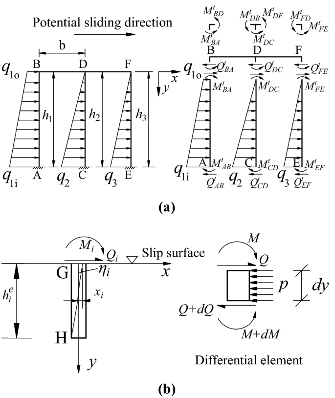

  

  Analytical models of a micropile group: a loaded segment; b embedded segment

• 2. Owing to the flexural rigidity of the roof plate that is much higher than that of a micropile in practice, the connections at the pile tops with the roof plate are assumed to be rigid.

• 3. The embedded segment of a micropile in the group is assumed as Winkler foundation beam [31]. Considering the homogeneous soil slope in Fig. 2, the foundation coefficient can be assumed to increase linearly with depth from zero at the ground surface.

• 4. The restraint condition at the bottom of the embedded segment of a micropile in the group is assumed as free.

• 5. The micropile group is assumed to be axisymmetric out of plane. The net thrust force on a micropile group is averagely divided to each loaded segment of the three column micropiles out of plane.

Based on the first assumption, the simplified analysis model of the loaded segment of a micropile group can be illustrated in Fig. 3a. Then, Eq. (10) can be derived according to structural mechanics [32]. Equation (11a) can be obtained in light of the static equilibrium conditions for joint B, D, F, and the roof plate. Meanwhile, according to the equilibrium conditions of the loaded segments of the three micropiles, Eq. (11b) can be obtained

$$\left. \begin{aligned} M^{l}_{AB} &= - \frac{{q_{1o} h_{1}^{2} }}{30} - \frac{{q_{1i} h_{1}^{2} }}{20} + 2\frac{{E_{1} I_{1} }}{{h_{1} }}\psi_{\text{B}} - 6\frac{{E_{1} I_{1} }}{{h_{1} }}\frac{\Delta }{{h_{1} }} + 6\frac{{E_{1} I_{1} }}{{h_{1} }}\frac{{x_{1} }}{{h_{1} }} + 4\frac{{E_{1} I_{1} }}{{h_{1} }}\eta_{1} \hfill \\ M^{t}_{BA} &= \frac{{q_{1o} h_{1}^{2} }}{20} + \frac{{q_{1i} h_{1}^{2} }}{30} + 4\frac{{E_{1} I_{1} }}{{h_{1} }}\psi_{B} - 6\frac{{E_{1} I_{1} }}{{h_{1} }}\frac{\Delta }{{h_{1} }} + 6\frac{{E_{1} I_{1} }}{{h_{1} }}\frac{{x_{1} }}{{h_{1} }} + 2\frac{{E_{1} I_{1} }}{{h_{1} }}\eta_{1} \hfill \\ M^{t}_{BD} &= 4\frac{{E_{2} I_{2} }}{b}\psi_{\text{B}} + 2\frac{{E_{2} I_{2} }}{b}\psi_{\text{D}} \hfill \\ M^{t}_{DB} &= 2\frac{{E_{2} I_{2} }}{b}\psi_{\text{B}} + 4\frac{{E_{2} I_{2} }}{b}\psi_{\text{D}} \hfill \\ M^{t}_{CD} &= - \frac{{q_{2} h_{2}^{2} }}{20} + 2\frac{{E_{1} I_{1} }}{{h_{2} }}\psi_{\text{D}} - 6\frac{{E_{1} I_{1} }}{{h_{2} }}\frac{\Delta }{{h_{2} }} + 6\frac{{E_{1} I_{1} }}{{h_{2} }}\frac{{x_{2} }}{{h_{2} }} + 4\frac{{E_{1} I_{1} }}{{h_{2} }}\eta_{2} \hfill \\ M^{t}_{DC} &= \frac{{q_{2} h_{2}^{2} }}{30} + 4\frac{{E_{1} I_{1} }}{{h_{2} }}\psi_{\text{D}} - 6\frac{{E_{1} I_{1} }}{{h_{2} }}\frac{\Delta }{{h_{2} }} + 6\frac{{E_{1} I_{1} }}{{h_{2} }}\frac{{x_{2} }}{{h_{2} }} + 2\frac{{E_{1} I_{1} }}{{h_{2} }}\eta_{2} \hfill \\ M^{t}_{DF} &= 4\frac{{E_{2} I_{2} }}{b}\psi_{\text{D}} + 2\frac{{E_{2} I_{2} }}{b}\psi_{\text{F}} \hfill \\ M^{t}_{FD} &= 2\frac{{E_{2} I_{2} }}{b}\psi_{\text{D}} + 4\frac{{E_{2} I_{2} }}{b}\psi_{\text{F}} \hfill \\ M^{t}_{EF} &= - \frac{{q_{3} h_{3}^{2} }}{20} + 2\frac{{E_{1} I_{1} }}{{h_{3} }}\psi_{\text{F}} - 6\frac{{E_{1} I_{1} }}{{h_{3} }}\frac{\Delta }{{h_{3} }} + 6\frac{{E_{1} I_{1} }}{{h_{3} }}\frac{{x_{3} }}{{h_{3} }} + 4\frac{{E_{1} I_{1} }}{{h_{3} }}\eta_{3} \hfill \\ M^{t}_{FE} & = \frac{{q_{3} h_{3}^{2} }}{30} + 4\frac{{E_{1} I_{1} }}{{h_{3} }}\psi_{\text{F}} - 6\frac{{E_{1} I_{1} }}{{h_{3} }}\frac{\Delta }{{h_{3} }} + 6\frac{{E_{1} I_{1} }}{{h_{3} }}\frac{{x_{3} }}{{h_{3} }} + 2\frac{{E_{1} I_{1} }}{{h_{3} }}\eta_{3} \hfill \\ \end{aligned} \right\},$$

(10)

where M^t is the bending moment of the loaded segment of a micropile group, in which the first subscript denotes the location of the internal forces and the second one represents the structural member of the group. q is the net linear load due to slope thrust force on the loaded segment of a micropile group, in which the subscripts 2 and 3 denote the middle and the leading row, respectively, and the subscripts 1o and 1i represent the top and tip of the trailing row’s loaded segment, respectively. h is the length of a micropile above potential slip surface, where subscript i denote row number of micropiles in one group. b is the spacing between adjacent rows (in plane) in one micropile group. E₁I₁ is the flexural rigidity of a micropile. E₂I₂ is the equivalent flexural rigidity of the roof plate. ψ is the rotation displacement of points on the roof plate, in which subscripts B, D, and F denote the joint B, D, and F in Fig. 3. Δ is the translation displacement of the rigid roof plate. x is the lateral displacement of micropiles at the slip surface, in which subscript i = 1, 2, and 3 denote the trailing, middle and leading row of the group, respectively. η is the rotation displacement of the micropile cross section at the slip surface, in which subscripts 1, 2, and 3 denote point A, C, and E in Fig. 3, respectively.

$$\left. \begin{array}{l} M^{t}_{BA} + M^{t}_{BD} = 0 \hfill \\ M^{t}_{DB} + M^{t}_{DC} + M^{t}_{DF} = 0 \hfill \\ M^{t}_{FD} + M^{t}_{FE} = 0 \hfill \\ Q^{t}_{BA} + Q^{t}_{DC} + Q^{t}_{FE} = 0 \hfill \\ \end{array} \right\}$$

(11a)

where Q^t is the shear force of the loaded segment of a micropile group, in which the first subscript denotes the location of the internal forces and the second one represents the structural member of the group.

$$\left. \begin{array}{l} Q_{BA}^{t} = \left( { - M_{AB}^{t} - M_{BA}^{t} - q_{1o} h_{1}^{2} /3 - q_{1i} h_{1}^{2} /6} \right)/h_{1} \hfill \\ Q_{AB}^{t} = Q_{BA}^{t} + \left( {q_{1o} + q_{1i} } \right)h_{1} /2 \hfill \\ Q_{AB}^{t} \left( y \right) = q_{1o} \left( {h_{1} - y} \right) + \left( {q_{1i} - q_{1o} } \right)\left( {h_{1} - y} \right)^{2} /\left( {2h_{1} } \right) + Q_{BA}^{t} \hfill \\ M_{AB}^{t} \left( y \right) = - M_{BA}^{t} - Q_{BA}^{t} \left( {h_{1} - y} \right) - q_{1o} \left( {h_{1} - y} \right)^{2} /2 - \left( {q_{1i} - q_{1o} } \right)\left( {h_{1} - y} \right)^{3} /\left( {6h_{1} } \right) \hfill \\ Q_{DC}^{t} = \left( { - M_{CD}^{t} - M_{DC}^{t} - q_{2} h_{2}^{2} /6} \right)/h_{2} \hfill \\ Q_{CD}^{t} = Q_{DC}^{t} + q_{2} h_{2} /2 \hfill \\ Q_{CD}^{t} \left( y \right) = q_{2} \left( {h_{2} - y} \right)^{2} /\left( {2h_{2} } \right) + Q_{DC}^{t} \hfill \\ M_{CD}^{t} \left( y \right) = - M_{DC}^{t} - Q_{DC}^{t} \left( {h_{2} - y} \right) - q_{2} \left( {h_{2} - y} \right)^{3} /\left( {6h_{2} } \right) \hfill \\ Q_{FE}^{t} = \left( { - M_{EF}^{t} - M_{FE}^{t} - q_{3} h_{3}^{2} /6} \right)/h_{3} \hfill \\ Q_{EF}^{t} = Q_{FE}^{t} + q_{3} h_{3} /2 \hfill \\ Q_{EF}^{t} \left( y \right) = q_{3} \left( {h_{3} - y} \right)^{2} /\left( {2h_{3} } \right) + Q_{FE}^{t} \hfill \\ M_{EF}^{t} \left( y \right) = - M_{FE}^{t} - Q_{FE}^{t} \left( {h_{3} - y} \right) - q_{3} \left( {h_{3} - y} \right)^{3} /\left( {6h_{3} } \right) \hfill \\ \end{array} \right\},$$

(11b)

where y represents the distance from any cross section to the top of each micropile (see Fig. 3a).

Substituting Eq. (10) into (11a), one obtains Eq. (12):

$$\left[ \begin{aligned} \left( {4\frac{{E_{1} I_{1} }}{{h_{1} }} + 4\frac{{E_{2} I_{2} }}{b}} \right){\kern 1pt} {\kern 1pt} {\kern 1pt} {\kern 1pt} {\kern 1pt} {\kern 1pt} {\kern 1pt} {\kern 1pt} {\kern 1pt} {\kern 1pt} {\kern 1pt} {\kern 1pt} 2\frac{{E_{2} I_{2} }}{b}{\kern 1pt} {\kern 1pt} {\kern 1pt} {\kern 1pt} {\kern 1pt} {\kern 1pt} {\kern 1pt} {\kern 1pt} {\kern 1pt} {\kern 1pt} {\kern 1pt} {\kern 1pt} {\kern 1pt} {\kern 1pt} {\kern 1pt} {\kern 1pt} {\kern 1pt} {\kern 1pt} {\kern 1pt} 0{\kern 1pt} {\kern 1pt} {\kern 1pt} {\kern 1pt} {\kern 1pt} {\kern 1pt} {\kern 1pt} {\kern 1pt} {\kern 1pt} {\kern 1pt} {\kern 1pt} {\kern 1pt} {\kern 1pt} {\kern 1pt} - 6\frac{{E_{1} I_{1} }}{{h_{1}^{2} }} \hfill \\ 2\frac{{E_{2} I_{2} }}{b}{\kern 1pt} {\kern 1pt} {\kern 1pt} {\kern 1pt} {\kern 1pt} {\kern 1pt} {\kern 1pt} \left( {4\frac{{E_{1} I_{1} }}{{h_{2} }} + 8\frac{{E_{2} I_{2} }}{b}} \right){\kern 1pt} {\kern 1pt} {\kern 1pt} {\kern 1pt} {\kern 1pt} {\kern 1pt} {\kern 1pt} {\kern 1pt} {\kern 1pt} 2\frac{{E_{2} I_{2} }}{b}{\kern 1pt} {\kern 1pt} {\kern 1pt} {\kern 1pt} {\kern 1pt} {\kern 1pt} {\kern 1pt} {\kern 1pt} - 6\frac{{E_{1} I_{1} }}{{h_{2}^{2} }} \hfill \\ {\kern 1pt} {\kern 1pt} {\kern 1pt} 0{\kern 1pt} {\kern 1pt} {\kern 1pt} {\kern 1pt} {\kern 1pt} {\kern 1pt} {\kern 1pt} {\kern 1pt} {\kern 1pt} {\kern 1pt} {\kern 1pt} {\kern 1pt} {\kern 1pt} {\kern 1pt} {\kern 1pt} {\kern 1pt} 2\frac{{E_{2} I_{2} }}{b}{\kern 1pt} {\kern 1pt} {\kern 1pt} {\kern 1pt} {\kern 1pt} {\kern 1pt} {\kern 1pt} {\kern 1pt} {\kern 1pt} {\kern 1pt} {\kern 1pt} {\kern 1pt} \left( {4\frac{{E_{1} I_{1} }}{{h_{3} }} + 4\frac{{E_{2} I_{2} }}{b}} \right){\kern 1pt} {\kern 1pt} {\kern 1pt} {\kern 1pt} {\kern 1pt} {\kern 1pt} {\kern 1pt} {\kern 1pt} {\kern 1pt} {\kern 1pt} {\kern 1pt} - 6\frac{{E_{1} I_{1} }}{{h_{3}^{2} }} \hfill \\ {\kern 1pt} - 6\frac{{E_{1} I_{1} }}{{h_{1}^{2} }}{\kern 1pt} {\kern 1pt} {\kern 1pt} {\kern 1pt} {\kern 1pt} {\kern 1pt} {\kern 1pt} {\kern 1pt} {\kern 1pt} {\kern 1pt} {\kern 1pt} {\kern 1pt} {\kern 1pt} {\kern 1pt} {\kern 1pt} {\kern 1pt} {\kern 1pt} {\kern 1pt} {\kern 1pt} - 6\frac{{E_{1} I_{1} }}{{h_{2}^{2} }}{\kern 1pt} {\kern 1pt} {\kern 1pt} {\kern 1pt} {\kern 1pt} {\kern 1pt} {\kern 1pt} {\kern 1pt} {\kern 1pt} {\kern 1pt} {\kern 1pt} {\kern 1pt} {\kern 1pt} {\kern 1pt} {\kern 1pt} {\kern 1pt} {\kern 1pt} {\kern 1pt} {\kern 1pt} {\kern 1pt} - 6\frac{{E_{1} I_{1} }}{{h_{3}^{2} }}{\kern 1pt} {\kern 1pt} {\kern 1pt} {\kern 1pt} {\kern 1pt} {\kern 1pt} {\kern 1pt} {\kern 1pt} {\kern 1pt} {\kern 1pt} {\kern 1pt} {\kern 1pt} {\kern 1pt} {\kern 1pt} 12E_{1} I_{1} \left( {\frac{1}{{h_{1}^{3} }} + \frac{1}{{h_{2}^{3} }} + \frac{1}{{h_{3}^{3} }}} \right) \hfill \\ \end{aligned} \right]\left[ \begin{aligned} \psi_{B} \\ \psi_{D} \\ \psi_{F} \\ \Delta \\ \end{aligned} \right]{ = }\left[ \begin{aligned} g_{1} \\ g_{2} \\ g_{3} \\ g_{4} \\ \end{aligned} \right]{\kern 1pt}$$

(12)

where

$$\begin{aligned} g_{1} & = - \left( {\frac{{q_{1o} h_{1}^{2} }}{20} + \frac{{q_{1i} h_{1}^{2} }}{30} + 6\frac{{E_{1} I_{1} }}{{h_{1} }}\frac{{x_{1} }}{{h_{1} }} + 2\frac{{E_{1} I_{1} }}{{h_{1} }}\eta_{1} } \right), \\ g_{2} & = - \left( {\frac{{q_{2} h_{2}^{2} }}{30} + 6\frac{{E_{1} I_{1} }}{{h_{2} }}\frac{{x_{2} }}{{h_{2} }} + 2\frac{{E_{1} I_{1} }}{{h_{2} }}\eta_{2} } \right), \\ g_{3} & = - \left( {\frac{{q_{3} h_{3}^{2} }}{30} + 6\frac{{E_{1} I_{1} }}{{h_{3} }}\frac{{x_{3} }}{{h_{3} }} + 2\frac{{E_{1} I_{1} }}{{h_{3} }}\eta_{3} } \right), \\ g_{4} & = \frac{{7q_{1o} h_{1} }}{20} + \frac{{3\left( {q_{1i} h_{1} + q_{2} h_{2} + q_{3} h_{3} } \right)}}{20} + 12E_{1} I_{1} \left( {\frac{{x_{1} }}{{h_{1}^{3} }} + \frac{{x_{2} }}{{h_{2}^{3} }} + \frac{{x_{3} }}{{h_{3}^{3} }}} \right) \\ & \quad + 6E_{1} I_{1} \left( {\frac{{\eta_{1} }}{{h_{1}^{2} }} + \frac{{\eta_{2} }}{{h_{2}^{2} }} + \frac{{\eta_{3} }}{{h_{3}^{2} }}} \right). \\ \end{aligned}$$

So, we can obtain expressions of ψ_B, ψ_D, ψ_F and Δ from Eq. (12). Further, the formula of moments and shear forces of each micropile at the slip surface can be derived according to Eqs. (10)–(12). However, the formulas of these internal forces are involved in ten unknown variables q_1o, q_1i, q₂, q₃, x₁, x₂, x₃, η₁, η₂, and η₃, which can be solved using ten independent equations.

Based on the second assumption, the joint rotation displacements of points B, D, and F (see Fig. 3a) are identical and we can obtain two independent equations:

$$\left\{ \begin{aligned} \psi_{B} = \psi_{D} \hfill \\ \psi_{D} = \psi_{F} \hfill \\ \end{aligned} \right..$$

(13)

Based on the third assumption, the analysis model for the embedded segment of the micropile is shown in Fig. 3b. According to the static equilibrium conditions of the differential element of the embedded segment, differential equations for internal forces are described as Eq. (14a):

$$\left. \begin{array}{l} Q + {\text{d}}Q - Q + p{\text{d}}y = 0 \Rightarrow \frac{{{\text{d}}Q}}{{{\text{d}}y}} = - p \hfill \\ M + {\text{d}}M - M + \left( {p{\text{d}}y} \right)\frac{{{\text{d}}y}}{2} - Q{\text{d}}y = 0 \Rightarrow \frac{{{\text{d}}M}}{{{\text{d}}y}} = Q \hfill \\ \end{array} \right\}.$$

(14a)

Also based on the third assumption, the pressure of Winkler foundation acted on a pile along its shaft can be written as:

$$p = kxB_{\text{p}} = myxB_{\text{p}} ,$$

(14b)

where k is the lateral Winkler foundation coefficient, B_p is the calculation width of a micropile, which is assumed to be the pile diameter, and m is the proportionality factor of lateral Winkler foundation coefficient varying with depth.

According to the Bernoulli beam theory [32], one obtains

$$E_{1} I_{1} \frac{{{\text{d}}^{2} x}}{{{\text{d}}y^{2} }} = M\left( y \right).$$

(14c)

Combining Eqs. (14a)–(14c), one obtains:

$$E_{1} I_{1} \frac{{{\text{d}}^{4} x}}{{{\text{d}}y^{4} }} + myxB_{\text{p}} = 0{\kern 1pt} .$$

(14d)

Then, according to the solving method of the differential equations, Eq. (14d) can be solved by the power series [33]. By further arrangement, the bending moments and shear forces of the embedded segment can be written as:

$$\begin{aligned} \frac{{M_{i}^{e} }}{{\alpha^{2} EI}} = x_{i} A_{Mi} + \frac{{\eta_{i} }}{\alpha }B_{Mi} + \frac{{M_{i} }}{{\alpha^{2} EI}}C_{Mi} + \frac{{Q_{i} }}{{\alpha^{3} EI}}D_{Mi} , \hfill \\ \frac{{Q_{i}^{e} }}{{\alpha^{3} EI}} = x_{i} A_{Qi} + \frac{{\eta_{i} }}{\alpha }B_{Qi} + \frac{{M_{i} }}{{\alpha^{2} EI}}C_{Qi} + \frac{{Q_{i} }}{{\alpha^{3} EI}}D_{Qi} , \hfill \\ \end{aligned}$$

(15)

where α is the deformation coefficient of a micropile, α = (mB_p/E₁I₁)^1/5. Q_i, M_i is the shear force and bending moment at the top of the embedded segment of a micropile group, in which subscript i (i = 1, 2 and 3) denotes the number of each pile row. A, B, C, and D are the calculation coefficients of internal forces, in which the former subscripts M and Q denote bending moment and shear force calculation, respectively, and the latter subscript i (i = 1, 2 and 3) denotes the number of each pile row in a micropile group. These calculation coefficients of internal forces are given as follows:

$$\left\{ \begin{aligned} & A_{Mi} = \sum\limits_{k = 1}^{\infty } {\left( { - 1} \right)^{k} \frac{{\left( {5k - 4} \right)!!}}{{\left( {5k - 2} \right)!}}\left( {\alpha y_{i}^{e} } \right)^{5k - 2} } \hfill \\& B_{Mi} = \sum\limits_{k = 1}^{\infty } {\left( { - 1} \right)^{k} \frac{{\left( {5k - 3} \right)!!}}{{\left( {5k - 1} \right)!}}\left( {\alpha y_{i}^{e} } \right)^{5k - 1} } \hfill \\& C_{Mi} = 1 + \sum\limits_{k = 1}^{\infty } {\left( { - 1} \right)^{k} \frac{{\left( {5k - 2} \right)!!}}{{\left( {5k} \right)!}}{\kern 1pt} {\kern 1pt} \left( {\alpha y_{i}^{e} } \right)^{5k} } \hfill \\& D_{Mi} = \alpha y + \sum\limits_{k = 1}^{\infty } {\left( { - 1} \right)^{k} \frac{{\left( {5k - 1} \right)!!}}{{\left( {5k + 1} \right)!}}{\kern 1pt} {\kern 1pt} \left( {\alpha y_{i}^{e} } \right)^{5k + 1} } \hfill \\& A_{Qi} = \sum\limits_{k = 1}^{\infty } {\left( { - 1} \right)^{k} \frac{{\left( {5k - 4} \right)!!}}{{\left( {5k - 3} \right)!}}\left( {\alpha y_{i}^{e} } \right)^{5k - 3} } \hfill \\& B_{Qi} = \sum\limits_{k = 1}^{\infty } {\left( { - 1} \right)^{k} \frac{{\left( {5k - 3} \right)!!}}{{\left( {5k - 2} \right)!}}\left( {\alpha y_{i}^{e} } \right)^{5k - 2} } \hfill \\& C_{Qi} = \sum\limits_{k = 1}^{\infty } {\left( { - 1} \right)^{k} \frac{{\left( {5k - 2} \right)!!}}{{\left( {5k - 1} \right)!}}{\kern 1pt} {\kern 1pt} \left( {\alpha y_{i}^{e} } \right)^{5k - 1} } \hfill \\& D_{Qi} = 1 + \sum\limits_{k = 1}^{\infty } {\left( { - 1} \right)^{k} \frac{{\left( {5k - 1} \right)!!}}{{\left( {5k} \right)!}}{\kern 1pt} {\kern 1pt} \left( {\alpha y_{i}^{e} } \right)^{5k} } \hfill \\ \end{aligned} \right.,$$

(15a)

where ye i is the y coordinate of any cross section (see Fig. 3b).

Based on the fourth assumption, we can get six independent equations [Eq. (16)] about the ten variables:

$$\left\{ \begin{aligned} M_{i}^{b} = 0 \left( {i = 1,2,3} \right) \hfill \\ Q_{i}^{b} = 0 \left( {i = 1,2,3} \right) \hfill \\ \end{aligned} \right.,$$

(16)

where $Q_{i}^{b}$ and $M_{i}^{b}$ are the shear force and bending moment at the bottom of micropiles, in which subscript i (i = 1, 2 and 3) denotes the pile row number. Q^b and M^b satisfy Eq. (16a) according to Eq. (15):

$$\left\{ \begin{aligned} \frac{{M_{i}^{b} }}{{\alpha^{2} E_{1} I_{1} }} = x_{i} A_{Mi} + \frac{{\eta_{i} }}{\alpha }B_{Mi} + \hfill \\ \frac{{M_{i} }}{{\alpha^{2} E_{1} I_{1} }}C_{Mi} + \frac{{Q_{i} }}{{\alpha^{3} E_{1} I_{1} }}D_{Mi} \hfill \\ \frac{{Q_{i}^{b} }}{{\alpha^{3} E_{1} I_{1} }} = x_{i} A_{Qi} + \frac{{\eta_{i} }}{\alpha }B_{Qi} + \hfill \\ \frac{{M_{i} }}{{\alpha^{2} E_{1} I_{1} }}C_{Qi} + \frac{{Q_{i} }}{{\alpha^{3} E_{1} I_{1} }}D_{Qi} \hfill \\ \end{aligned} \right.,$$

(16a)

where A, B, C, and D can be obtained from Eq. (15a) with setting $y_{i}^{e}$ as $h_{i}^{e}$ ($h_{i}^{e}$ is the length of a micropile below potential slip surface, in which subscript i denotes row number of micropiles in one group).

Based on the continuity of internal forces of a micropile, the internal forces at the bottom of the loaded segment should be equal to those at the top of the embedded segment. Thus, one obtains:

$$M_{1} = M^{t}_{AB} ,M_{2} = M^{t}_{CD} ,M_{3} = M^{t}_{EF} ,$$

(16b)

$$Q_{1} = Q^{t}_{AB} ,Q_{2} = Q^{t}_{CD} ,Q_{3} = Q^{t}_{EF} .$$

(16c)

At the same time, the sum of the moments and shear forces of the three micropiles at the slip surface should be equal to those obtained using LAM mentioned above for the micropile group, respectively. Based on the fifth assumption, we can also get the other two independent equations:

$$\left\{ \begin{aligned} && M^{t}_{AB} + M^{t}_{CD} + M^{t}_{EF} = \frac{{M^{u} \cdot S}}{3} \hfill \\ && Q^{t}_{AB} + Q^{t}_{CD} + Q^{t}_{EF} = \frac{P \cdot S}{3} \hfill \\ \end{aligned} \right.,$$

(17)

where S is the center-to-center spacing between adjacent two micropile groups.

So the ten variables q_1o, q_1i, q₂, q₃, x₁, x₂, x₃, η₁, η₂, and η₃ can be determined by Eqs. (13), (16) and (17). Naturally, the internal forces of each micropile of the group can be easily calculated. The computation procedure for responses of a micropile group can be carried out via a computer program such as Matlab. The corresponding flow chart is schematically illustrated in Fig. 4, which can be elaborated as follows:

Fig. 4

Computation flow chart for responses of a micropile group

Step 1::

Calculation of net thrust force on the group

Input main physical properties of the slope, the local surcharge on the slope top and design factor of safety of the piled slope (β₁, β₂, κ₁, κ₂, H, Y; σ, τ, L₁, L_F; n, and F_s), calculate P and h_a using Eq. (9), and calculate M^u using Eq. (7).

Step 2::

Calculation of shear force and bending moment at the ends of the loaded segment of a micropile group

Obtain the expression of [Ψ_B, Ψ_D, Ψ_F, Δ]^T using Eq. (12), and gain the expression of $M_{AB}^{t}$, $M_{BA}^{t}$, $M_{CD}^{t}$, $M_{DC}^{t}$, $M_{EF}^{t}$, and $M_{FE}^{t}$ by substituting the expression of [Ψ_B, Ψ_D, Ψ_F, Δ]^T into Eq. (10); then obtain the expression of $Q_{AB}^{t}$, $Q_{BA}^{t}$, $Q_{CD}^{t}$, $Q_{DC}^{t}$, $Q_{EF}^{t}$, and $Q_{FE}^{t}$ by substituting the expression of $M_{AB}^{t}$, $M_{BA}^{t}$, $M_{CD}^{t}$, $M_{DC}^{t}$, $M_{EF}^{t}$, and $M_{FE}^{t}$ into Eq. (11b).

Step 3::

Calculation of shear force and bending moment at the top of the embedded segment

Based on the results from step 2, calculate the expression of M₁, M₂, M₃, Q₁, Q₂, and Q₃ by substituting the expression of $M_{AB}^{t}$, $M_{CD}^{t}$, $M_{EF}^{t}$, $Q_{AB}^{t}$, $Q_{CD}^{t}$, and $Q_{EF}^{t}$into Eqs. (16b) and (16c).

Step 4::

Calculation of the ten unknown variables q_1o, q_1i, q₂, q₃, x₁, x₂, x₃, η₁, η₂, and η₃

Based on the results from step 3, substitute the expression of M₁, M₂, M₃, Q₁, Q₂, and Q₃ into Eq. (16a) and then substitute Eq. (16a) into (16); based on the results from step 2, substitute the expression of [Ψ_B, Ψ_D, Ψ_F, Δ]^T into Eq. (13), and substitute the expression of $M_{AB}^{t}$, $M_{CD}^{t}$, $M_{EF}^{t}$, $Q_{AB}^{t}$, $Q_{CD}^{t}$, and $Q_{EF}^{t}$, P and M^u into Eq. (17); then calculate the 10 unknown variables q_1o, q_1i, q₂, q₃, x₁, x₂, x₃, η₁, η₂, and η₃ using Eqs. (13), (16) and (17).

Step 5::

Calculation of responses of the loaded segment of a micropile group

Substitute the solutions of q_1o, q_1i, q₂, q₃, x₁, x₂, x₃, η₁, η₂, and η₃ into Eq. (10), then obtain $M_{AB}^{t}$, $M_{CD}^{t}$, $M_{EF}^{t}$, $Q_{AB}^{t}$, $Q_{CD}^{t}$, and $Q_{EF}^{t}$; further substitute these solutions into Eq. (11b), and figure out $M_{AB}^{t} (y)$, $M_{CD}^{t} (y)$, $M_{EF}^{t} (y)$, $Q_{AB}^{t} (y)$, $Q_{CD}^{t} (y)$, and $Q_{EF}^{t} (y)$.

Step 6::

Calculation of responses of the embedded segment of a micropile group

Based on the results from steps 4 and 5, substitute the solutions of $M_{AB}^{t}$, $M_{CD}^{t}$, $M_{EF}^{t}$, $Q_{AB}^{t}$, $Q_{CD}^{t}$, and $Q_{EF}^{t}$ into Eqs. (16b) and (16c), then gain M₁, M₂, M₃, Q₁, Q₂, and Q₃; then substitute the solutions of M₁, M₂, M₃, Q₁, Q₂, Q₃, x₁, x₂, x₃, η₁, η₂, and η₃ into Eq. (15), and determine $M_{i}^{e}$ and $Q_{i}^{e}$(i = 1, 2, 3).

Thus, internal forces of each pile in one group can be obtained.

3 Verifications

To demonstrate the rationality of the proposed method, a large-scale geotechnical laboratory model test and corresponding 3D-numerical simulation have been conducted.

A piled slope test model with 0.94 m width out of plane is shown in Figs. 5a and 6a. There are three micropile groups with 0.2 m center-to-center spacing out of plane arranged in the test model (see Fig. 5b). The slope soil was prepared with fine quartz sand, pottery clay, and water at the ratio of 50:3:2. The roof plates of the model micropile groups were made of hardwood plates, and the model piles with 0.67 m length were made of hollow aluminum tubes with 8 and 7 mm outer and inner diameters, respectively. The main properties of the model slope soil and micropile group are shown in Table 1.

Fig. 5

Layout of the test model: a cross section; b plane diagram; c layout of measuring points; d arrangement of micropiles in the middle group

Fig. 6

Model test photos: a side view; b arrangement of soil pressure cells on the sides of the piles; c front view

Table 1 Main properties of the model slope soil and micropile group

As shown in Figs. 5c and 6b, three model piles in the middle group (see Fig. 5d) were instrumented with 42 strain gauges along their shafts for measuring their bending moments (see Eq. (18)). And 48 soil pressure cells were laid out on both sides of the piles for measuring slope pressure on the piles (see Fig. 6b). To measure lateral displacements of the slope and the micropile group, three dial gauges were installed at the crest, toe of the slope and the front side of the roof plate, respectively (see Fig. 6c).

The loading test was conducted by placing concrete blocks on the top of the model slope (see Figs. 5a, 6a). The surcharge is 24.7 kPa in the test to observe responses of the piled slope distinctly.

Figure 7 shows net slope pressure on the leading, middle, and trailing loaded segments of the micropiles in the instrumented group. It can be seen that distributions of the net slope pressure are bidirectional and getting weaker from top to bottom along the shaft of the loaded segments of the piles. The corresponding analysis results of a 3D-numerical simulation using FLAC^3D for the test model (see Fig. 8) are also given in Fig. 7. The net slope pressure on the measured micropiles in the test is close to those obtained using the numerical simulation method (NSM).

Fig. 7

Net slope pressure on the loaded segments of the measured micropiles

Fig. 8

3D-Numerical simulation model of the test slope

In addition, Fig. 9 shows the critical slip surface of the model slope computed using the proposed method and the NSM with shear strength reduction strategy and yielded a factor of safety value of 1.31. The corresponding net thrust force per unit width P is calculated to be 0.785 kN/m using the proposed method. It can be seen that the critical slip surfaces of the piled slope obtained by the two methods are almost identical.

Fig. 9

Critical slip surface of the model slope

Bending moments and shear forces of micropiles obtained by the model test, the proposed method, and the NSM are also shown in Fig. 10a–f, in which the measured bending moments M_i and shear forces Q_i of the three model piles are obtained by Eq. (18) [32]:

$$\left\{ \begin{aligned} M_{i} &= E_{1} I_{1} \left( {\varepsilon_{i + } - \varepsilon_{i - } } \right)/D \hfill \\ Q_{i} &= \left( {{\text{d}}M_{i} /{\text{d}}y} \right) \approx \left( {M_{i + 1} - M_{i} } \right)/\left( {2d} \right) \hfill \\ \end{aligned} \right.,$$

(18)

where ε_i+ and ε_i− are strain measured on the front and rear side of model piles, respectively, in which subscript i (i = 1–7) denotes row number of micropiles in one group. D is the outer diameter of the model piles. d is the distance between two adjacent strain measuring points (see Fig. 5c).

Fig. 10

Bending moment and shear force of micropiles: a, c, and e bending moment of the leading, middle, and trailing micropile, respectively; b, d, and f shear force of the leading, middle, and trailing micropile, respectively

It can be seen from Fig. 10 that the distribution tendency of bending moment and shear force of each measured micropile observed in the test is similar to that computed using the proposed method and the NSM. But it should be noted that the analytical calculation and numerical simulation are carried out under the condition that the piled slope is in the critical state with a factor of safety. However, the model test of the piled slope is not in the critical state due to the actual loading limitation in the laboratory. Therefore, there are distinct differences of the values of the internal forces between the test and the proposed method as well as the NSM. Additionally, although the results obtained by the proposed method and NSM are relatively close, there are local differences of the results between the two computation methods. The possible reason is that some assumptions introduced in the proposed method are likely not identical with the conditions in the related numerical models.

For the leading and trailing pile, the maximum positive bending moment above the slip surface by the proposed method is nearly located at the middle point of the loaded segment (see Fig. 10a, e). Meanwhile, the maximum negative bending moment below the slip surface by the proposed method is nearly located at the upper third point of the embedded segment. The values and locations of the two maximum bending moments obtained using the proposed method are fairly close to those by the NSM.

For the middle micropile, the maximum positive bending moment above the slip surface by the proposed method is at the top of the pile (see Fig. 10c). Its location is above that by the NSM, and its value is higher than that by the NSM. The location of the maximum negative bending moment by the proposed method is also nearly located at the upper third point of the embedded segment. And both its location and value are close to those by the NSM.

But for the three micropiles, the maximum shear forces obtained by the proposed method and the NSM are both located nearly at the slip surface (Fig. 10b, d, f). And the value of the maximum shear force by the proposed method is about 40% larger than that by the NSM for the leading and trailing micropiles and about 15% less than that by the NSM for the middle micropile.

In general, bending moments and shear forces obtained by the proposed method agree well with those by the NSM. However, it is noteworthy that the values by the model test are far less than those computed by the other two methods. The reason lies in the fact that in the model test they are captured under the condition that the piled slope is far away from the limit state. But the related theoretical or numerical values are computed in the limit state of the piled slope with the factor of safety 1.31.

4 Parameter Study and Discussion

The practical soil slope [18] reinforced with traditional stabilizing piles by Austilo et al. shown in Fig. 11 is taken herein as an example. The slope height is 13.7 m, and the slope angle is 30°. Unit weight, cohesion, and internal friction angle of the slope soil are 19.63 kN/m³, 23.94 kPa, and 10°, respectively. The slope is reinforced here with micropile groups 7.8 m away from the slope toe. Meanwhile, a micropile group consists of nine micropiles in three rows and three columns connected by a roof plate at their tops (see Fig. 12). Three 40 mm-diameter steel bars are used for each micropile. The elastic modulus and equivalent flexural rigidity of a single micropile are 200 GPa and 276.46 kN m², respectively. Each micropile hole has a diameter of 130 mm and is injected with M20 cement mortar. The center-to-center spacing between two adjacent groups is 3 m. The spacing between two micropiles in one group is 0.6 m in plane and 0.5 m out of plane. The roof plate has 0.2 m cantilever length over border micropiles of the group.

Fig. 11

A slope example

Fig. 12

Layout of micropile groups in the slope example

The net thrust force P under the design safety factor 1.2 is 105.2 kN/m computed by the proposed method. And the corresponding slip surface of the piled slope is simultaneously obtained (see Fig. 11). Therefore, both the loaded and embedded segment lengths of the micropiles are adopted as 6.1 m.

4.1 Flexural Rigidity of a Micropile

Figure 13 shows internal forces of the trailing micropile in the practical example under four various flexural rigidities including 0.41 E₁I₁ (E₁I₁ = 276.46 kN m² mentioned above), 0.66 E₁I₁, 1.00 E₁I₁, and 2.44 E₁I₁ which are corresponding to 32, 36, 40, and 50 mm diameter steel bars, respectively. The results indicate that bending moment of the pile increases marginally with increasing its flexural rigidity (see Fig. 13a), and the shear force decreases slightly with the increase of the flexural rigidity (see Fig. 13b). But distribution characteristics of the internal forces are almost not changed with flexural rigidity of the micropile.

Fig. 13

Effect of flexural rigidity of a micropile on its internal forces: a bending moment; b shear force

4.2 Micropile Length

To simply discuss the effect of micropile length on its internal forces, embedding ratio (denoted by R_h) is defined herein as a ratio of the embedded segment length over the loaded segment length of the micropile. Figure 14 shows internal forces of the trailing micropile in the example under five various embedding ratios R_h including 0.5, 0.8, 1.0, 1.2, and 1.5, respectively. Both the bending moment and the shear force of the micropile are nearly not influenced by the ratio (see Fig. 14a, b). The result is somewhat different from that of the traditional stabilizing pile with a large cross section. The reason is that the micropile is generally of much higher slenderness ratio than the traditional pile.

Fig. 14

Effect of micropile length on its internal forces: a bending moment; b shear force

4.3 Micropile Spacing in Plane

As shown in Fig. 15a, b, R_S is the ratio of micropile spacing in plane over the pile diameter, the ratio R_S has almost no effect on bending moment and shear force of the trailing micropile in the example. It is because relative rigidity of the roof plate E₂I₂/b is far more than that of micropiles E₁I₁/h_i (i = 1, 2, 3), and the relative rigidity of the roof plate influences to great extent internal forces of micropiles according to structural mechanics principle when the ratio R_S is altered from 3.0 to 8.0 [see Eqs. (10)–(12)].

Fig. 15

Effect of micropile spacing in plane on its internal forces: a bending moment; b shear force

4.4 Micropile Numbers

Figure 16 shows that internal forces of the trailing micropile in the example are remarkably influenced by total numbers of micropiles in one group including 2 × 2, 2 × 3, and 3 × 3 layout, respectively. Bending moment and shear force of the micropile are decreasing as expected with increasing the pile numbers (see Fig. 16a, b). But the distribution mode of internal forces is hardly varied with the pile numbers.

Fig. 16

Effect of micropile numbers in one group on its internal forces: a bending moment; b shear force

5 Conclusions

A new simplified analytical method for combined stabilizing micropile groups used to reinforce slopes or landslides is presented. Internal forces of a micropile group can be calculated by dividing it into two parts with the boundary of the design slip surface. The upper and lower parts can be regarded as a plane rigid frame model and an elastic foundation beam model, respectively.

For a specified factor of safety of a piled slope, resistance at the design slip surface provided by a micropile group can be computed via a series of formulas derived in light of kinematical limit analysis method. The resistance should then be adopted as boundary conditions used in analyzing the upper part of the micropile group.

Flexural rigidity of a micropile and total numbers of micropiles in one group have a substantial effect on bending moment and shear force of the micropile. In particular, the internal forces are relatively sensitive to pile numbers in a group.

However, micropile length and micropile spacing in plane in a group have both little effects on internal forces of the micropile, which is rather different from traditional stabilizing piles with large cross section because of fairly high flexibility of the micropile.

Appendix

In Fig. 2, there are following geometric relationships:

$$\frac{X}{{r_{0} }} = \frac{H}{{r_{0} }} \cdot \frac{{\sin \left( {\beta - \beta^{\prime}} \right)}}{{\sin \beta \sin \beta^{\prime}}},$$

(19)

where X is the horizontal distance from the slope toe to the intersection between the log-spiral slip line and the ground outside the toe. H is the height of the slope. β and β′ are dip angles of line JN and JN′ in Fig. 2, respectively.

$$H\cot \beta = \kappa_{1} H\cot \beta_{1} + \kappa_{2} H\cot \beta_{2} + Y,$$

(20)

where κ and β are the ratio of local slope height over the whole slope height and the dip angle of the slope face, respectively. And the subscripts 1 and 2 denote the upslope and downslope in Fig. 2, respectively. Y is the width of bench of the slope.

$$\kappa_{1} + \kappa_{2} { = }1,$$

(21)

$$\frac{L}{{r_{0} }} = \frac{{\sin \left( {\theta_{\text{h}} - \theta_{0} } \right)}}{{\sin \left( {\theta_{\text{h}} + \delta } \right)}} - \frac{{\sin \left( {\theta_{\text{h}} + \beta^{\prime}} \right)}}{{\sin \left( {\theta_{\text{h}} + \delta } \right)\sin \left( {\beta^{\prime} - \delta } \right)}}\left[ {{\text{e}}^{{\left( {\theta_{\text{h}} - \theta_{0} } \right)\tan \varphi_{\text{f}} }} \cdot \sin \left( {\theta_{\text{h}} + \delta } \right) - \sin \left( {\theta_{0} + \delta } \right)} \right].$$

(22)

According to the concept of the gravity work rate [26], the coefficients of the gravity work rate can be derived and expressed as follows:

$$f_{1} = \frac{{\left( {3\tan \varphi_{\text{f}} \cos \theta_{\text{h}} + \sin \theta_{\text{h}} } \right) \cdot {\text{e}}^{{3\left( {\theta_{\text{h}} - \theta_{0} } \right)\tan \varphi_{\text{f}} }} - \left( {3\tan \varphi_{\text{f}} \cdot \cos \theta_{0} + \sin \theta_{0} } \right)}}{{3\left( {1 + 9\tan^{2} \varphi_{\text{f}} } \right)}},$$

(23)

$$f_{2} = \frac{1}{6}\frac{L}{{r_{0} }}\left[ {2\cos \theta_{0} - \frac{L}{{r_{0} }}\cos \delta } \right]\sin \left( {\theta_{0} + \delta } \right){\kern 1pt} ,$$

(24)

$$\begin{aligned} f_{3} &= \frac{1}{6}\kappa_{1} \frac{H}{{r_{0} }}\left( {2\left( {\cos \theta_{0} - \frac{L}{{r_{0} }}\cos \delta } \right) - \kappa_{1} \frac{H}{{r_{0} }}\cot \beta_{1} } \right) \hfill \\ &\quad \cdot \left[ {\left( {\cos \theta_{0} - \frac{L}{{r_{0} }}\cos \delta } \right) + \cot \beta_{1} \left( {\sin \theta_{0} + \frac{L}{{r_{0} }}\sin \delta } \right)} \right], \hfill \\ \end{aligned}$$

(25)

$$f_{4} = \frac{1}{6} \cdot \frac{Y}{{r_{0} }} \cdot \left( {\kappa_{1} \frac{H}{{r_{0} }} + \frac{L}{{r_{0} }}\sin \delta + \sin \theta_{0} } \right) \cdot \left( \begin{aligned} &2\cos \theta_{0} - 2\frac{L}{{r_{0} }}\cos \delta \hfill \\ &\quad - 2\kappa_{1} \frac{H}{{r_{0} }}\cot \beta_{1} - \frac{Y}{{r_{0} }} \hfill \\ \end{aligned} \right),$$

(26)

$$f_{5} = \frac{1}{6}\kappa_{2} \frac{H}{{r_{0} }}\left[ \begin{aligned} &\left( {{\text{e}}^{{\left( {\theta_{\text{h}} - \theta_{0} } \right)\tan \varphi_{\text{f}} }} \cdot \cos \theta_{\text{h}} + \frac{X}{{r_{0} }}} \right) \hfill \\ &\quad + \cot \beta_{2} \cdot \left( {\frac{H}{{r_{0} }} + \frac{L}{{r_{0} }}\sin \delta + \sin \theta_{0} } \right) \hfill \\ \end{aligned} \right] \cdot \left[ \begin{aligned} &2\left( {{\text{e}}^{{\left( {\theta_{\text{h}} - \theta_{0} } \right)\tan \varphi_{\text{f}} }} \cdot \cos \theta_{\text{h}} + \frac{X}{{r_{0} }}} \right) \hfill \\ &\quad + \kappa_{2} \frac{H}{{r_{0} }}\cot \beta_{2} \hfill \\ \end{aligned} \right],$$

(27)

$$f_{6} = \frac{1}{6}\frac{X}{{r_{0} }}\left( {2{\text{e}}^{{\left( {\theta_{\text{h}} - \theta_{0} } \right)\tan \varphi_{\text{f}} }} \cdot \cos \theta_{\text{h}} + \frac{X}{{r_{0} }}} \right) \cdot \left( {\frac{H}{{r_{0} }} + \frac{L}{{r_{0} }}\sin \delta + \sin \theta_{0} } \right).$$

(28)

References

.Bruce DA, Juran I (1997) Drilled and grouted micropiles: state-of-practice review, volume II: design, vol no. FHWA-RD-96-017. United States Department of Transportation, USA
Xiao SG, Cui K, Zhou DP, Feng J (2009) Analysis of a new combined micropile structure for preventing slope slippage and its application in a practical project. In: ICCTP 2009, ASCE, pp 1–11. http://doi.org/10.1061/41064(358)5
Bruce DA, Dimillio AF, Juran I (1997) Micropiles: the state of practice part I: characteristics, definitions and classifications. Ground Improv 1(1):25–35. https://doi.org/10.1680/gi.1997.010104
Moayed RZ, Naeini SA (2012) Imrovement of loose sandy soil deposits using micropiles. KSCE J Civ Eng 16(3):334–340. https://doi.org/10.1007/s12205-012-1390-2
Isam S, Hassan A, Mhamed S (2012) 3D elastoplastic analysis of the seismic performance of inclined micropiles. Comput Geotech 39:1–7. https://doi.org/10.1016/j.compgeo.2011.08.006
Galloway J, Mjelde J, Allen B (2013) Ship loader platforms using a pile/micropile system. In: Ports ‘13: triennial international conference, ASCE, pp 735–744. http://doi.org/10.1061/9780784413067.076
Moon JS, Lee S (2016) Static skin friction behavior of a single micropile in sand. KSCE J Civ Eng 20(5):1793–1805. https://doi.org/10.1007/s12205-016-0918-2
Cantoni R, Collotta T, Ghionna VN, Moretti PC (1989) A design method for reticulated micropile structures in sliding slopes. Ground Eng 22(4):41–47
Juran I, Benslimane A, Bruce DA (1996) Slope stabilization by micropile reinforcement. In: Proceedings of the 7th international symposium on landslides, Trondheim, pp 1718–1726
Loehr JE, Ang EC, Parra JR, Bowders JJ (2004) Design methodology for stabilizing slopes using recycled plastic reinforcement. In: Yegian MK, Kavazanjian E (eds) Proceedings of geo-trans 2004: geotechnical engineering for transportation projects, ASCE, pp 723–731. http://doi.org/10.1061/40744(154)59
Sun SW, Zhu BZ, Wang JC (2013) Design method for stabilization of earth slopes with micropiles. Soils Found 53(4):487–497. https://doi.org/10.1016/j.sandf.2013.06.002
Xiang B, Zhang L, Zhou LR, He YY, Zhu L (2014) Field lateral load tests on slope-stabilization grouted pipe pile groups. J Geotech Geoenviron Eng 141(4):04014124. https://doi.org/10.1061/(ASCE)GT.1943-5606.0001220
Deng DP, Li L, Zhao LH (2017) Limit-equilibrium method for reinforced slope stability and optimum design of antislide micropile parameters. Int J Geomech 17(2):06016019. https://doi.org/10.1061/(ASCE)GM.1943-5622.0000722
Poulos HG (1971) Behavior of laterally loaded piles: II-pile groups. J Soil Mech Found Div 97(5):733–751
Poulos HG (1973) Analysis of piles in soil undergoing lateral movement. J Soil Mech Found Div 99(5):391–406
Lee CY, Hull TS, Poulos HG (1995) Simplified pile-slope stability analysis. Comput Geotech 17(1):1–16. https://doi.org/10.1016/0266-352X(95)91300-S
Poulos HG (1995) Design of reinforcing piles to increase slope stability. Can Geotech J 32(5):808–818. https://doi.org/10.1139/t95-078
Ausilio E, Conte E, Dente G (2001) Stability analysis of slopes reinforced with piles. Comput Geotech 28(8):591–611. https://doi.org/10.1016/S0266-352X(01)00013-1
Guo WD (2009) Nonlinear response of laterally loaded piles and pile groups. Int J Numer Anal Methods Geomech 33(7):879–914. https://doi.org/10.1002/nag.746
Guo WD (2014) Nonlinear response of laterally loaded rigid piles in sliding soil. Can Geotech J 52(7):903–925. https://doi.org/10.1139/cgj-2014-0168
Xiao SG (2017) A simplified approach for stability analysis of slopes reinforced with one row of embedded stabilizing piles. Bull Eng Geol Environ 76(4):1371–1382. https://doi.org/10.1007/s10064-016-0934-y
Xiao SG, He H, Zeng JX (2016) Kinematical limit analysis for a slope reinforced with one row of stabilizing piles. Math Probl Eng 2016:1–15. https://doi.org/10.1155/2016/5463929
Ito T, Matsui T, Hong WP (1981) Design method for stabilizing piles against landslide-one row of piles. Soils Found 21(1):21–37
Hassiotis S, Chameau JL, Gunaratne M (1997) Design method for stabilization of slopes with piles. J Geotech Geoenvironm Eng 123(4):314–323. https://doi.org/10.1061/(ASCE)1090-0241(1997)123:4(314)
Zeng S, Liang R (2002) Stability analysis of drilled shafts reinforced slope. J Jpn Geotech Soc 42(2):93–102
Chen WF (1975) Limit analysis and soil plasticity. Elsevier, Amsterdam
Yu HS, Salgado R, Sloan SW, Kim JM (1998) Limit analysis versus limit equilibrium for slope stability. J Geotech Geoenviron Eng 124(1):1–11
Li XP, He SM, Wang CH (2006) Stability analysis of slopes reinforced with piles using limit analysis method. In: Advances in earth structures: research to practice, pp 105–112. http://doi.org/10.1061/40863(195)8
Li XP, Pei XJ, Gutierrez M, He SM (2012) Optimal location of piles in slope stabilization by limit analysis. Acta Geotech 7(3):253–259. https://doi.org/10.1007/s11440-012-0170-y
Zienkiewicz OC, Humpheson C, Lewis RW (1975) Associated and nonassociated visco-plasticity and plasticity in soil mechanics. Géotechnique 25(4):671–689
Jones G (1997) Analysis of beams on elastic foundation. Thomas Telford, London. https://doi.org/10.1680/aoboef.25752.0002
Krenk S, Høgsberg J (2013) Statics and mechanics of structures. Springer, Dordrecht. https://doi.org/10.1007/978-94-007-6113-1
Constanda C (2013) Differential equations. Springer, New York. https://doi.org/10.1007/978-1-4614-7297-1
Acknowledgements
The research was supported by the National Natural Science Foundation of China (Grant Nos. 51278430 and 51578466) and the Program for New Century Excellent Talents in University (NCET-13-0976). Besides, the authors would also like to appreciate the anonymous reviewers giving useful suggestion in improving this article.
Author information
Authors and Affiliations
Corresponding author