Optimal Sizing of Distributed Energy Resources in a Microgrid System with Highly Penetrated Renewables

Abstract

Economic dispatch (ED) of a grid connected and renewable integrated microgrid system is considered in this paper. Two wind farms take the renewable energy sources (RES) into consideration. A parameter worst-case-transaction-cost which arises due to the stochastic availability and uncontrollable nature of wind farms is also emphasised and efforts have been taken to minimize it too. Hence the paper’s focus into split objective functions and the generation costs and the worst case transaction costs are optimised separately and also the net microgrid cost is optimized as a whole. Two different cases with highly varying transaction prices are studied. Two meta-heuristic soft computing algorithms are applied for optimization and a comparative analysis among them is studied. Numerical results are tabulated to justify the effectiveness of the novel approach.

1 Introduction

A microgrid is a collection of electrical loads, communication facilities, control units and generating units that are spread within a small geographical location. The distributed energy resources (DERs) included in the microgrid may be micro turbines, fuel cells, reciprocating engines, or any of a number of alternate power sources (Hatziargyriou et al. 2007). Countries such as the USA, Germany, Greece, Japan have seen the distribution of microgrids and have benefited from them (Barnes 2007). The effective management of a microgrid system in order to supply the required power without facing shortcomings and with a minimized economy is the problem gaining attention (Koutsopoulos and Tassiulas 2012; Khodayar et al. 2012). The Energy Management system makes decisions regarding the best use of the DERs for producing electric power and heat, based upon the heat requirements of the local equipment, the weather conditions, the price of electric power, the cost of fuel and many other considerations.

Extensive literature survey on microgrid energy management has provided insight about the different methodologies employed so far to solve these problems. The demand for electrical power is intensifying at a very fast rate, which, in turn has caused a rapid growth of the real-time market price of electricity. To accommodate these high rising demands, electrical power sectors are growing up significantly. In India most of the electrical energy is derived from fossil fuel based power plants. In this framework, smart grids and microgrids are the key in the near future where a decentralization of energy generation is expected. An advantage of these type of grids is that the balance between energy generation, storage, and consumption can be realized most efficiently. This reduces the need for centralized communication, enables autonomous operations of increasingly smaller sections of the distribution grid and decreases the losses by distant distribution. From the point of view of a microgrid energy management system, economic scheduling of generation devices, storage systems and loads is a crucial problem. Performance of an optimization process is necessary to minimize the operating costs while several operational constraints are taken into account.

The cost of fuel is a major part of the running expenses of various small power stations and this will be enhanced if the efficiency of the plants is to be improved. Hence, the minimization of operating costs has attracted a great deal of attention from the power engineers. Mostly conventional classical based dual decomposition optimization techniques were employed to solve the basic energy management based microgrid problems. However, these approximations resulted in solution of reduced accuracy and hence, huge revenue loss over time. Moreover, in most of the above mentioned algorithms, the numbers of control parameters (which control the performance of the algorithm) are large. Therefore, a time consuming control parameter tuning procedure is required before applying these algorithms to a specific optimization problem

Various loads and the DERs are controlled and maintained by the microgrid energy manager (MGEM). All the DERs and loads have dedicated local controllers that coordinate with the MGEM for the timely operation of resources in a distributed fashion. This disciplined and distributed fashioned functioning of microgrids face the challenge when the uncertainty and stochastic nature of RES come into view. Economic dispatch and unit commitment of a microgrid is done in Stluka et al. (2011) without considering the stochastic nature of RES. Considering the Wei bull distribution for wind speed an ED problem deals with minimization of risk of over-estimation and under-estimation of wind in Hetzer et al. (2008). For a single period, probabilistic study of supply of power is studied with an ED problem involving RES in Liu and Xu (2010). Authors in Guan et al. (2010) considered the stochastic availability nature of demand and PV generation while minimizing the microgrid net cost. Robust scheduling problems with fine incorporated for the uncertainty of supply and demand without considering DSM have been studied in Bertsimas et al. (2013). Some heuristic algorithms are implemented by the authors in Jiang and Low (2011) and Zhao and Zeng (2012) to perform demand side management in RES integrated microgrids. Model predictive control is used for planning problem of a microgrid with DS in Jin and Ghosh (2011). The unreliable and time varying nature of RES is neglected and then distributed algorithm is used to supply a given load including DER in Dom (2011). Considering a microgrid with a single wind farm and no DS, a worst-case transaction based energy management is done in Zhang and Gatsis (2012). Energy management of co-operative microgrids was performed in Lahon and Gupta (2017) to minimize the net operating cost which includes the cost of distributed generation and worst case transaction cost. In Govardhan and Roy (2012) a microgrid with wind turbine, PV array, diesel engine, fuel cell and micro-turbine are studied. The proposed cost functions considered are the cost of the emissions NO_x, SO₂ and CO₂, operating and maintenance cost as well as start-up costs of different sources. The total operating cost of the microgrid is minimized with the help of Ant Bee Colony optimization technique. The isolation niche immune genetic algorithm (INIGA) is used in Liao (2013) to confirm the accuracy and validity of the mathematic model through some actual examples. This method is then compared with some other optimization approaches that are usually applied to solve the energy management and optimization operation problem to show the superiority and usability of the approach mentioned in it. Authors in Shi et al. (2015) designed a distributed energy management strategy (DEMS) based on IEC 61850 bounded by system operational constraints. This DEMS was then implemented on a real microgrid system of China consisting of a photo-voltaic system, wind turbines (WT), diesel generators and battery storage device. Three different optimization techniques viz. genetic algorithm (GA), particle swarm optimization (PSO) and honey bee mating optimization (HBMO) were used by authors in Ahmadnia and Tafehi (2017) to improve the voltage stability margin for seven different scenarios of a microgrid system which consisted of DERs like PV, WT, STATCOM and capacitors. A multi-objective optimization method was presented in Chen et al. (2018) to jointly optimize the planning and operation of a grid-connected microgrid system that included PV, WT and DS. The author used fuzzy satisfaction maximization method for five different scenarios of the microgrid system. A memory based GA (MGA) technique was used in Askarzadeh (2017) to optimize the sharing of power generation among the DERs of a microgrid system to minimize its operating cost. This proposed technique was then compared with GA and two variants of PSO to prove its superiority.

Evolvement of soft computing tools, which are not restricted by the complexity of system models, inspired the research workers to apply them in the field of power system optimization. The versatile properties and attractive performance of genetic algorithm (GA), particle swarm optimization (PSO) and differential evolution (DE) over a wide range of benchmark functions have inspired the many researchers to implement these algorithms for solving energy management issues of microgrids involving optimal costs and load scheduling. Nevertheless, GA, PSO and DE have their own list of disadvantages too. The very basic disadvantage of GA is its unguided mutation. The mutation operator in GA functions like adding a randomly generated number to a parameter of an individual of the population. This is the only reason for the very slow convergence of genetic algorithm. DE suffers from unstable convergence and easily drops down to regional optimum. Likewise, PSO also drops down to regional optimum and has untimely convergence. In addition, multiplicity of population is not enough in PSO. Also, some time is consumed in tuning the control parameters present in all of the aforementioned optimization techniques.

However, there is also a recently developed, simple yet powerful meta-heuristic algorithm called symbiotic organisms search (SOS). In this algorithm the symbiotic interaction tactics that organisms generally use to survive in an ecosystem are simulated. SOS showed better results in various fields of power engineering where optimization is of prime concern. In Das and Bhattacharya (2016), SOS has been implemented in short term hydro thermal scheduling problems and better results were obtained. SOS algorithm has been implemented in Datta et al. (2016) to determine the optimal coordination of directional over current relays. It is worth mentioning that SOS outperformed the various optimization techniques considered for comparative study in this case too. SOS also gave better results than some prior optimization techniques when implemented for real power loss minimization in Balachennaiah and Suryakalavathi (2015).

To avoid the suboptimal solution and to accelerate the convergence speed, the theory of quasi-oppositional based learning (Q-OBL) is integrated with original SOS and used to solve the microgrid energy management based problem. The success of QOSOS algorithm is established by comparing the dynamic performances of concerned microgrid system with those obtained by SOS and some recently published algorithms available in the literature. Furthermore, the robustness and sensitivity are analysed for the concerned microgrid system to judge the efficacy of the proposed QOSOS approach.

2 Mathematical formulation of Microgrid Energy Management System

Let us consider a grid-connected microgrid system comprised of conventional (fossil fuel) generators, RES facilities (wind-farms) supported by DS units supplying power to both elastic and inelastic loads (Fig. 1). The modelling of various DERs for the optimal scheduling of the microgrid system is done in the next sub-sections.

Fig. 1

Architecture of a typical microgrid

2.1 Load Demand Model

There are generally two types of loads: inelastic loads and elastic loads. Inelastic loads are the ones which are fixed and their demand should be satisfied at all times. For e.g. hospitals, schools and colleges, government and administrative offices, etc. Elastic loads are those type of loads whose demand may be compromised in case of power shortage and can be scheduled as per time horizon. There are two types of elastic loads:

• 1. Say, the N number of class-1 dispatchable loads have power consumption $P_{{D_{n} }}^{t} \in [P_{{D_{n} }}^{\hbox{min} } ,P_{{D_{n} }}^{\hbox{max} } ]$, where $n \in {\rm N}: = \{ 1, \ldots ,N\}$, and $t \in \tau$. For this class of elastic loads, the consumption of power varies directly with the utility of the end user. The increasingly concave utility function of the nth dispatchable load, $U_{{D_{n} }}^{t} (P_{{D_{n} }}^{t} )$(Chen et al. 2010). The utility of the class-1 type of loads is calculated using the equation

  $$U_{n} (P_{{D_{n} }} ) = c_{n} P_{{D_{n} }}^{2} + d_{n} P_{{D_{n} }}$$

  (1)

• 2. The Q number of class-2 type of elastic loads denoted by $q \in Q: = \{ 1,2, \ldots\,Q\}$ with power consuming capability ranging from $P_{{E_{q} }}^{\hbox{min} }$ to $P_{{E_{q} }}^{\hbox{max} }$, and permissible energy desired $E_{q}$ is attained from the start time $S_{q}$ to termination time $T_{q}$ (Mohsenian-Rad et al. 2010). Plug-in hybrid electric vehicles (PHEVs) can be considered as a better illustration of this type of load. The time-varying function on which the qth load will operate is a concave function $U_{{E_{q} }}^{t} (P_{{E_{q} }}^{t} )$ and is calculated with the relation:

  $$U_{{E_{q} }}^{t} (P_{{E_{q} }}^{t} ): = \pi_{q}^{t} P_{{E_{q} }}^{t}$$

  (2)

  with weights $\{ \pi_{q}^{t} \}$ decreasing in t from slots $S_{q}$ to $T_{q}$.

2.2 Distributed Storage Model

For stable operation to balance any instantaneous mismatch in active power, efficient DS must be used. Distributed storage enhances the overall performance of microgrid systems in many ways. Firstly, it stabilizes and permits DG units to run at a constant and stable output, despite load fluctuations. Secondly, it provides the ride-through capability when there are dynamic variations of primary energy (such as those of sun, wind, and hydropower sources). It also permits DG to seamlessly operate as a dispatchable unit. Moreover, energy storage can benefit power systems by damping peak surges in electricity demand. In addition to all of these a DS counters momentary power disturbances and provides outage ride-through while backup generators respond. The property of a DS to reserve energy for future demand is of utmost importance.

Let $B_{j}^{t}$ be the energy stored at the jth battery when the time slot t ends. Suppose the energy which was initially available is $B_{j}^{0}$ while $B_{j}^{\hbox{max} }$ indicates maximum energy of the battery, such that $0 < B_{j}^{t} < B_{j}^{\hbox{max} } ,j \in J: = \{ 1,2 \ldots J\}$. Let $P_{{B_{j} }}^{t}$ be considered as the exchanged power to or from the jth storage device during time slot $t$ which causes charging $(P_{{B_{j} }}^{t} \le 0)$ or discharging $(P_{{B_{j} }}^{t} \ge 0)$ of the battery. Energy stored in the battery can be defined as:

$$B_{j}^{t} = B_{j}^{t - 1} + P_{{B_{j} }}^{t}$$

(3)

Constraints of $P_{{B_{j} }}^{t}$ are:

• 1. The discharging and charging of the battery obeys the equation:

  $$\begin{aligned} \begin{array}{l} P_{{B_{j} }}^{\hbox{min} } \le P_{{B_{j} }}^{t} \le P_{{B_{j} }}^{\hbox{max} } \hfill \\ - \eta_{j} B_{j}^{t - 1} \le P_{{B_{j} }}^{t} \hfill \\ \end{array} \end{aligned}$$

  (4)

  where $P_{{B_{j} }}^{\hbox{min} }$ < 0, $P_{{B_{j} }}^{\hbox{max} }$ > 0, and $\eta_{j} \in (0,1]$ is the efficiency of the battery j.

• 2. Final stored energy at any instant of time is also limited so that DS can be used for future scheduling horizons. This limit is represented as $B_{j}^{T} \ge B_{j}^{\hbox{min} }$.

  The lifetime of the DS can be maximized by employing a storage cost $H_{j}^{t} (B_{j}^{t} )$ so that the stored energy maintains a specific level of charge (Vytelingum et al. 2011; Alimisis and Hatziargyriou 2013). To validate greater value of power exchange one can even select $H_{j}^{t} (B_{j}^{t} ) \equiv 0$ altogether.

2.3 Generation Cost of Conventional Generators

Let $P_{{G_{m} }}$ be the power output of the mth conventional fossil fuelled generator. Then the generator cost function which is quadratic in nature is represented by the equation:

$$C_{m} P_{{G_{m} }} = a_{m} P_{{G_{m} }}^{2} + b_{m} P_{{G_{m} }}$$

(5)

where a_m and b_m are the generator cost coefficients.

Hence the generation cost of the microgrid system is the sum of the generation costs of the conventional fossil-fuelled generators and the storage devices minus the utility of dispatchable loads and can be mathematically formulated as:

$$F_{1} = \sum\limits_{t = 1}^{T} {\left( {\sum\limits_{m = 1}^{M} {C_{m}^{t} (P_{{G_{m} }}^{t} ) - \sum\limits_{n = 1}^{N} {U_{{D_{n} }}^{t} - \sum\limits_{q = 1}^{Q} {U_{{E_{q} }}^{t} (P_{{E_{q} }}^{t} ) + \sum\limits_{j = 1}^{J} {H_{j}^{t} (B_{j}^{t} )} } } } } \right)}$$

(6)

2.4 Worst-case Transaction Cost

Let $W_{i}^{t}$ be the wind power generated by the ith RES facility (hereafter wind farm) for the time period t. Further, let w comprise $W_{i}^{t}$, i.e. $w: = \{ W_{1}^{1} , \,\ldots W_{1}^{T} , \,\ldots W_{I}^{1} ,\, \ldots W_{I}^{T} \}$. The combined power output from the wind farms when postulated for a period t within the time scheduling horizon can be expressed as:

$$\begin{aligned}\begin{array}{l} \underline{{W_{i}^{t} }} \le W_{i}^{t} \le \bar{W}_{i}^{t} \hfill \\ s.t.\;W_{s}^{\hbox{min} } \le \sum\limits_{i = 1}^{I} {W_{i}^{t} \le W_{s}^{\hbox{max} } } \hfill \\\end{array} \end{aligned}$$

(7)

where $\underset{\raise0.3em\hbox{$\smash{\scriptscriptstyle-}$}}{W}_{i}^{t}$ & $\bar{W}_{i}^{t}$ stands for the higher and lower limits of $W_{i}^{t}$ respectively. The total wind energy harvested over the region is bounded by $W_{s}^{\hbox{min} }$ and $W_{s}^{\hbox{max} }$ (Zhao and Zeng 2012) and the deterministic lower and upper bounds can be determined via inference schemes based on historical data (Pinson and Kariniotakis 2010).

Since the paper considers a microgrid operating in a grid connected mode, there exists a buying/selling mechanism between the main grid and microgrid. Let $P_{R}^{t}$ denote the net power delivered to the microgrid at time t from the renewable energy sources and the storage devices when the transaction mechanism is going on. The mathematical expression ($P_{R}^{t} - \sum\nolimits_{i = 1}^{I} {W_{i}^{t} } + \sum\nolimits_{j = 1}^{J} {P_{{B_{j} }}^{t} }$) calculates the shortage or surplus of energy. $\alpha^{t}$ is the cost price of purchasing power in case of deficit and $\beta^{t}$ is the selling price of the power when the microgrid yields an excess of it.

Worst-case-transaction cost can be mathematically expressed as:

$$F_{2} = \sum\limits_{t = 1}^{T} {\left( {\alpha^{t} \left[P_{R}^{t} - \sum\limits_{i = 1}^{I} {W_{i}^{t} } + \sum\limits_{j = 1}^{J} {P_{{B_{j} }}^{t} } \right]^{ + } - \beta^{t} \left[P_{R}^{t} - \sum\limits_{i = 1}^{I} {W_{i}^{t} } + \sum\limits_{j = 1}^{J} {P_{{B_{j} }}^{t} } \right]^{ - } } \right)}$$

(8)

where {$P_{R}^{t}$} collects $P_{R}^{t}$ for t = 1,2…T and $\{ {P_{{B_{j} }}^{t} } \}$ collects $\{ {P_{{B_{j} }}^{t} } \}$ for j = 1,2,…J, t = 1,2,…T.

2.5 Microgrid Energy Management Objective Function

Considering the cost of various DERs and the worst case transaction cost levied by the high penetration and dependability on the RES, the overall microgrid net social cost, which is to be minimized, can be mathematically represented as:

$$\begin{aligned} F = \mathop {\hbox{min} }\limits_{x} F_{1} + \mathop {\hbox{min} }\limits_{x} F_{2} \hfill \\ {\text{also}}\;F = \mathop {\hbox{min} }\limits_{x} \left( {F_{1} + F_{2} } \right) \hfill \\ \end{aligned}$$

(9a)

$$F = \mathop {\hbox{min} }\limits_{x} \left[ {\sum\limits_{t = 1}^{T} {\left( {\sum\limits_{m = 1}^{M} {C_{m}^{t} (P_{{G_{m} }}^{t} ) - \sum\limits_{n = 1}^{N} {U_{{D_{n} }}^{t} - \sum\limits_{q = 1}^{Q} {U_{{E_{q} }}^{t} (P_{{E_{q} }}^{t} ) + \sum\limits_{j = 1}^{J} {H_{j}^{t} (B_{j}^{t} )} } } } } \right)}+ \sum\limits_{t = 1}^{T} {\left( {\alpha^{t} [P_{R}^{t} - \sum\limits_{i = 1}^{I} {W_{i}^{t} } + \sum\limits_{j = 1}^{J} {P_{{B_{j} }}^{t} } ]^{ + } - \beta^{t} [P_{R}^{t} - \sum\limits_{i = 1}^{I} {W_{i}^{t} } + \sum\limits_{j = 1}^{J} {P_{{B_{j} }}^{t} } ]^{ - } } \right)} } \right]$$

(9b)

where x collects all the primal variables $\{ P_{{G_{m} }}^{t} ,P_{{D_{n} }}^{t} ,P_{{E_{q} }}^{t} ,P_{{B_{j} }}^{t} ,B_{j}^{t} ,P_{R}^{t} ,W_{i}^{t} \}$. Both the generation cost of the microgrid system $\left( {F_{1} } \right)$ and the worst case transaction cost $\left( {F_{2} } \right)$ are minimized separately and the overall microgrid net social cost is optimized as a whole using a bio-inspired meta-heuristic optimization technique and its improved variant. The results are then compared in a later section of this paper.

The above objective functions are subject to the constraints which are listed below:

2.5.1 Generation Limits

The conventional generator outputs should lie between its maximum and minimum limits.

$$P_{{G_{m} }}^{\hbox{min} } \le P_{{G_{m} }}^{t} \le P_{{G_{m} }}^{\hbox{max} }$$

(10a)

2.5.2 Ramp Up/Down Limits

The inequality constraints due to ramp rate limits for unit generation changes are given as:

For increase in generation

$$P_{{G_{m} }}^{t} - P_{{G_{m} }}^{t - 1} \le R_{{m,{\text{up}}}}$$

(10b)

For decrease in generation

$$P_{{G_{m} }}^{t - 1} - P_{{G_{m} }}^{t} \le R_{{m,{\text{down}}}}$$

(10c)

where R_m,up and R_m,down are the up ramp limit and the down ramp limit of the conventional generators respectively.

2.5.3 Spinning Reserve Constraint

The spinning reserve inequality for the conventional generator outputs at any time slot t denoted by SR^t is given as:

$$\sum\limits_{m = 1}^{M} {\left( {P_{{G_{m} }}^{\hbox{max} } - P_{{G_{m} }}^{t} } \right)} \ge SR^{t}$$

(10d)

2.5.4 Class-1 Loads Constraint

The power consumption of Class-1 type of elastic loads should lie between their minimum and maximum limits.

$$P_{{D_{n} }}^{\hbox{min} } \le P_{{D_{n} }}^{t} \le P_{{D_{n} }}^{\hbox{max} }$$

(10e)

2.5.5 Class-2 Loads Constraints

The power consumption of Class 2 type of loads should be within their upper and lower limits as assigned. Also, the total energy requirements which are targeted by the running duration of these loads must be equal to E_q. Mathematically,

$$\begin{aligned}\begin{array}{l} P_{{E_{q} }}^{\hbox{min} ,t} \le P_{{E_{q} }}^{t} \le P_{{E_{q} }}^{\hbox{max} ,t} \hfill \\ \sum\limits_{{t = S_{q} }}^{{T_{q} }} {P_{{E_{q} }}^{t} = E_{q} } \hfill \\ P_{{E_{q} }}^{\hbox{min} ,t} = P_{{E_{q} }}^{\hbox{max} ,t} = 0\quad {\text{for}}\;t \notin \left\{ {S_{q} , \ldots T_{q} } \right\} \hfill \\ \end{array}\end{aligned}$$

(10f)

2.5.6 Distributed Storage Constraints

Equation 7(h) and 7(i) bounds the stored energy and the amount of charging (discharging) between their maximum possible limits as

$$0 \le B_{j}^{t} \le B_{j}^{\hbox{max} } ,B_{j}^{T} \ge B_{j}^{\hbox{min} }$$

(10g)

$$P_{{B_{j} }}^{\hbox{min} } \le P_{{B_{j} }}^{t} \le P_{{B_{j} }}^{\hbox{max} }$$

(10h)

A fraction $\eta_{j}$ of the energy which is stored to be discharged is represented as

$$- \eta_{j} B_{j}^{t - 1} \le P_{{B_{j} }}^{t}$$

(10i)

$$B_{j}^{t} = B_{j}^{t - 1} + P_{{B_{j} }}^{t}$$

(10j)

2.5.7 Constraints for the Auxiliary Variable

The auxiliary variable should lie between the minimum and maximum limits as follows:

$$P_{R}^{\hbox{min} } \le P_{R}^{t} \le P_{R}^{\hbox{max} }$$

(10k)

2.5.8 Power Supply–demand Balance Equation

The sum of the generated powers of all units must be equal to sum of the power demanded by the load.

$$\sum\limits_{m = 1}^{M} {P_{{G_{m} }}^{t} + } P_{R}^{t} = L^{t} + \sum\limits_{n = 1}^{N} {P_{{D_{n} }}^{t} } + \sum\limits_{q = 1}^{Q} {P_{{E_{q} }}^{t} }$$

(10l)

In this present work the above formulated objective functions aims to minimize the overall microgrid net social cost. Different optimization techniques that are used to solve the objective functions are illustrated below in detail.

3 The Symbiotic Organisms Search Algorithm

Symbiotic organisms search is a relatively new powerful and meta-heuristic algorithm applied to optimize many mathematical and engineering problems (Cheng and Prayogo 2014). It works by simulating the symbiotic strategies acquired by the organisms among themselves to survive and be sustained in the ecosystem. The fact that SOS does not require any algorithm specific parameters makes it superior to many other meta-heuristic algorithms. The symbiotic relationships that are found in nature of three types viz. mutualism, commensalism and parasitism. These relationships are further formulated below and the SOS algorithm is developed as below:

3.1 Mutualism Phase

In the mutualism phase of SOS, both the species involved benefit. One common example is the relationship between honey bees and flowers (Fig. 2). The bees collect nectar from flowers and turn it into honey and hence benefit from the flowers. In this process the bees also carry the pollen grains from one flower to another and thus assist in pollination. This phase can be mathematically developed by the following equations:

Fig. 2

Honey bee and flower

$$X_{inew} = X_{i} + rand(0,1)*(X_{best}^{{}} - Mutual\_Vector*BF_{1} )$$

(11)

$$X_{jnew} = X_{j} + rand(0,1)*(X_{best}^{{}} - Mutual\_Vector*BF_{2} )$$

(12)

$$Mutual\_Vector = \frac{{X_{i} + X_{j} }}{2}$$

(13)

where X_i is an organism of the ith member of the ecosystem and X_j is randomly selected from the ecosystem to interact with X_i. rand(0,1) denotes a vector of random numbers. BF₁ and BF₂ denote the benefit factors and are kept either 1 or 2. Mutual_Vector represents the mutual relation between the organisms X_i and X_j.

3.2 Commensalism Phase

Commensalism is a relationship existing in nature between individuals of two species where one species gathers its food or one benefits from the other without harming or benefitting the latter. The remora fish, for instance, is always attached to the shark and eats the leftover food of a shark without harming or benefitting it. In this way there exists a commensalism relation between the shark and remora fish (Fig. 3). Similar to the mutualism phase, X_j is selected randomly to interact with X_i and a new organism X_inew can be calculated as:

$$X_{inew} = X_{i} + rand( - 1,1)*(X_{best} - X_{j} )$$

(14)

where (X_best− X_j) portrays the beneficial advantage provided by $X_{j}$ to help $X_{i}$ increase its survival advantage in ecosystem to the highest degree X_best in current organism.

Fig. 3

Remora fish and shark

3.3 Parasitism Phase

Parasitism is the name given to the relationship between two organisms in the ecosystem where one is harmed and the other benefits. The organism that benefits is called ‘parasite’ and the one that faces harm is called the ‘host’. Example can be taken of the deer tick (Fig. 4) which attaches to the host to suck its blood and thus benefits. But it also carries some Lyme disease, causing joint damage and kidney problems and also the animal suffers from lack of blood.

Fig. 4

Deer tick feeding on the blood of a host

In SOS, X_j is selected randomly to act as the host. Parasite_Vector is an artificial organism created in the search space. If fitness value of Parasite_Vector is better than X_j, it will replace organism X_j. And if the fitness value of X_j is better, it will have immunity and the Parasite_Vector will no longer survive in that ecosystem.

4 Quasi-Oppositional Based Learning

The idea of oppositional based learning (OBL) theory was originally introduced by Tizhoosh (2005). Later, it gained huge acceptability from the researchers in the field of computation intelligence. The basic aim of using OBL in the evolutionary computation is to enhance the solution accuracy and accelerate the convergence rate towards the global solution. It has a high probability to look after the optimization scheme to produce a suboptimal solution. In this process, current population and opposite number are simultaneously generated to produce better candidate solution. The theory of OBL is derived by defining three of its important mathematical attributes:

• (a) Opposite number: It is the mirror location of the candidate solution from the centre of search space. If X is a randomized initial candidate solution which lies in the interval [a,b], then the opposite number O_x in a d-dimensional space can be mathematically formulated as

  $$O_{{X_{j} }} = a_{j} + b_{j} - X_{j}$$

  (15)

  where $j = 1,2,3, \ldots d$ and $X_{j} = X_{1} ,X_{2} ,X_{3} , \ldots\,X_{d}$.

• (b) Quasi opposite number: the quasi-opposite number finds its position between the centre of search space and the opposite number and is often closer to the global optimum solution than the opposite number. Let ‘C’ be the centre of the search space. Mathematically $C = \frac{{a_{j} + b_{j} }}{2}$. Then the quasi-opposite number can be obtained by the following pseudo code:

  $$\begin{aligned} \begin{array}{l} {\textit{if}}(O_{x} < C) \hfill \\ QO_{x} = C + (O_{x} - C)*rand; \hfill \\ else \hfill \\ QO_{x} = O_{x} + (C - O_{x} )*rand; \hfill \\ end \hfill \\ \end{array} \end{aligned}$$

  (16)

  where $QO_{x}$ is the quasi-opposite number and $rand \in (0,1)$.

• (c) Jumping rate: This parameter is specifically needed to help the algorithm avoid any sub-optimal solution. The jumping rate also accelerates the algorithm attain a globally optimal solution. The value of jumping rate is normally selected between [0,0.6] and is mathematically defined as

  $$JR = JR_{\hbox{max} } - JR_{\hbox{min} } - (JR_{\hbox{max} } - JR_{\hbox{min} } )*\left(\frac{{fc_{\hbox{max} } - fc}}{{fc_{\hbox{max} } }}\right)$$

  (17)

  where ‘JR_max’ and ‘JR_min’ are the maximum and minimum values of jumping rate. ‘fc_max’ is the maximum number of function call and ‘fc’ is the number of function call at the present iteration.

5 Symbiotic organisms search (SOS) and quasi-oppositional symbiotic organisms search (QOSOS) applied to energy management problem

• Step 1: Formation of Ecosystem: The parameters considered for microgrid energy management include fuel cost-coefficients of conventional generators, power generation limits, ramp rate limits, power demand of various types of loads and limits of forecasted wind power. Also, the size of ecosystem i.e. the total number of organisms in the ecosystem (eco_size) and maximum iteration (max_iter) is set in this step.

• Step 2: Let X_i be the trial vector designating the ith organism of the initial ecosystem where P_i consists of generators outputs, class-1 loads, class-2 loads, an auxiliary variable and wind turbine outputs for 8 h intervals. Hence P_i can be represented as X_i = [Pg_i11,Pg_i12…Pg_i18,Pg_i21,Pg_i22…Pg_i28,Pg_i31,Pg_i32…Pg_i38,D_i11,D_i12….D_i18,D_i21,D_i22….D_i28,D_i31,D_i32….D_i38,D_i41,D_i42….D_i48,D_i51,D_i52….D_i58,D_i61,D_i62….D_i68,E_i11,E_i12…E_i18,E_i21,E_i22…E_i28,E_i31,E_i32…E_i38,E_i41,E_i42…E_i48,PtR_i1,PtR_i2…PtR_i8, W_i11,W_i12…W_i18,W_i21,W_i22…W_i28];

• Now for n number of members of the ecosystem (pop_size) i varies from i = 1, 2, 3….n. Hence the ecosystem matrix can be represented as

• $$X = \left[ \begin{aligned} X_{1} \hfill \\ X_{2} \hfill \\ X_{3} \hfill \\ \ldots \hfill \\ X_{n} \hfill \\ \end{aligned} \right]$$

• Step 3: Mutualism phase: Here i is initially set at 1, organism X₁ is matched to $X_{i}$ and organism $X_{j}$ is formed randomly from the ecosystem. In this case, X₂ is selected as $X_{j}$. Mutual_Vector is calculated using (13). Benefit Factors (1 and 2) are set at 2. Organism $X_{i}$ and $X_{j}$ are modified based on their mutual relationship using (11) and (12) and the constraints checking is done. Once it is found that $X_{i}$ and $X_{j}$ abide by the constraints, the fitness value is then accounted, if found better than the initial fitness value, we go to next step else we reject modified and keep the initial solution and proceed to next step.

• Step 4: Commensalism phase: Organism $X_{j}$($X_{j}$ ≠ $X_{i}$) is generated from the ecosystem on a random basis. New candidate solutions X1 are calculated using (14). Constraint checking is done and fitness value is calculated. Like the previous step, if fitness value of the modified organism in this step is better than the previous value then we go to the next step else the modified organism is rejected and the previous solution is kept before proceeding to the next step.

• Step 5: Parasitism phase: Organism $X_{j}$ ($X_{j}$ ≠ $X_{i}$) is randomly selected from the ecosystem. Parasite_Vector is formed by mutating $X_{i}$ in random dimensions using a random number within a given range. Constraint checking is done and fitness value is calculated. If Parasite_Vector is found better than the previously calculated fitness value, then the previous fitness value is replaced with the Parasite vector else the Parasite_Vector is rejected and then we proceed to the next step.

• Step 6: We proceed to step 2 if the current $X_{i}$ is not the last member of the ecosystem; otherwise we proceed to next step.

• Step 7: We stop if one of the termination criteria i.e. the maximum number of iterations is reached; otherwise we return to step 2 and start the next iteration.

Subsequently, the SOS algorithm was modified by incorporating the quasi-oppositional features in it and a modified and novel Quasi-Oppositional Symbiotic Organisms Search (QOSOS) algorithm was developed to minimize the same objective functions of the microgrid energy management problem. Figure 5 below shows the steps followed to minimize the microgrid net social cost using QOSOS.

Fig. 5

Flowchart of QOSOS

6 Numerical Results and Analysis

6.1 Description of the Test System

The considered microgrid consists of 3 conventional fossil-fuelled generators, 6 class-1 dispatchable loads, 4 class-2 dispatchable loads, 3 storage units and 2 renewable energy sources (wind farms). The time horizon spans for 8 h corresponding to the interval 4 PM–12 AM. Genetic Algorithm (GA), Particle swarm optimization (PSO) and Differential evolution (DE) were applied in Dey (2015) and have proved themselves better than the classical techniques applied for this work. In this section symbiotic organisms search (SOS) and proposed QOSOS techniques are implemented to evaluate their performance for solving microgrid energy management problems. The proposed algorithm to solve the energy management problem is coded in MATLAB R2013a and executed on a personal computer having 2.53 GHz core i3 processor with 3 GB RAM. The basic system parameters are listed in Table 1. Table 2 contains the various parameters of the conventional fossil fuelled generators. Tables 3 and 4 lists the operating limits and cost coefficients of class-1 and class-2 type of dispatchable loads respectively. The forecasted upper and lower limits of the wind farms, transaction prices for case A and case B and the values of inelastic loads are all listed in Table 5. The forecasted upper and lower limits of the wind farms are gathered from the MISO day-ahead wind forecast data (Zhang et al. 2013) and are rescaled to the order of 1 to 40 kWh, which, according to authors in Wu et al. (2011), is a typical wind power generation for a microgrid. Likewise, the hourly values of the fixed loads L^t which are listed in Table 5, are also collected and re-scaled from the daily report data provided by MISO in Federal Energy Regulatory Commission (2012). The program is run with different population sizes and 100 iterations for 50 trials using SOS. Benefit_Factor value is set at 2 and best result was found at a jumping rate of 0.45 while using QOSOS.

Table 1 Basic parameters of the microgrid system

Table 2 Conventional fossil-fuelled generators parameters

Table 3 Class 1 Dispatchable loads parameters

Table 4 Class-2 Dispatchable load parameters

Table 5 Boundary limits of the wind farms, fixed loads and real time transaction prices for both the cases

6.2 Comparative Study

• 1. Solution Quality: The minimized generation cost, worst transaction cost and microgrid net social cost for case A with the classical techniques used in literature, GA, PSO, DE, SOS and QOSOS algorithms are displayed in Table 6. It can be seen that proposed QOSOS gives the best and minimized solutions with $10.1022 for net generation cost, $7.9652 for worst transaction cost and $22.0051 for net microgrid cost. Similarly, for case B it can be seen from Table 7 that QOSOS yielded better solutions with $13.6527 for microgrid generation cost, $80.9699 for worst transaction cost and $135.9970 for microgrid net social cost respectively. From these results it is quite clear that proposed QOSOS algorithm gave better and least operation cost of the considered microgrid system compared to other algorithms. The optimal microgrid power schedules of both the cases are shown in Figs. 3 and 4. The stair steps include conventional power generation CG, and total elastic demands for classes 1 and 2 respectively. Quantity WORSTCASE denotes the total worst case wind energy at the respective time slot which is obtained with optimal $P_{R}^{t}$. A common observation from Figs. 3 and 4 is that the total conventional power generation varies with the same trend across t as the fixed load demand FIXEDLOADS, while the class-1 elastic load exhibits the opposite trend. Because the conventional generation and the power drawn from the main grid are limited, the optimal scheduling by solving (P2) dispatches less power for CLASS1 when FIXEDLOADS is large (from 6 P.M. to 10 P.M.), and vice versa. This behaviour indeed reflects the load shifting ability of the proposed design for the microgrid energy management. Furthermore, by comparing the two cases in Figs. 6 and 7 it is interesting to note that the difference between $P_{R}^{t}$ and WORSTCASE is the shortage power needed to purchase (if positive) or the surplus power to be sold (if negative).

  Table 6 Costs (in $) obtained for minimum value of objective functions (Case A)

  Table 7 Costs (in $) obtained for minimum value of objective functions (Case B)

  Fig. 6

  

  Optimal power schedule by QOSOS (Case A)

  Fig. 7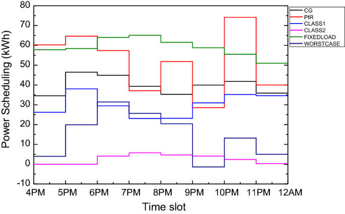

  

  Optimal power schedule by QOSOS (Case B)

• 2. Computational Efficiency: Table 8 highlights the low computational time and iteration counts taken by QOSOS to converge to the best solutions. It can be seen for case A, QOSOS takes 0.2150 iter/s and 0.2000 iter/s for case B. Also Figs. 5 and 6 show the convergence characteristics implying the fast convergence criteria of SOS and QOSOS than the rest of the soft computing techniques applied. It means that the time taken by QOSOS algorithm is much less and hence has significantly better computational efficiency to solve energy management problem. Also, Table 7 reflects the number of hits to optimum solution is far more with QOSOS than the other algorithms thus proving its robustness better than GA, PSO, DE and SOS used.

  Table 8 Solution quality analysis of various optimization techniques used for minimizing microgrid net social cost

7 Conclusion

Access to reliable source of electricity is a basic need for every individual. Implementation of microgrids can be considered as the most promising solution for rural or small area electrification. Moreover, providing a suitable means of power exchange between the microgrid and utility grid can be beneficial in terms of both objectives. An optimal strategy for supplying the required energy in an autonomous grid connected microgrid is developed in this paper by means of wind farms, distributed storage and conventional generators only. Based on the financial and operational perspective, the optimization problem was formulated and a new and modified algorithm QOSOS was presented to solve the optimization problem. The effectiveness of the proposed strategy in finding the optimum design was portrayed by the simulation results. The results also showed the proposed system is capable to meet electricity demand of microgrid. In addition, the paper focussed on minimizing the worst case transaction cost which arose due to the stochastic nature of RES. Finally, the accuracy and robustness of QOSOS compared with other conventional algorithms were shown. Since this paper mainly concentrated on cost minimization of the hybrid energy system, involvement of other RES and their reliability check can be a subject of future research (Figs. 7, 8, 9).

Fig. 8

Convergence characteristics of net microgrid cost during Case A

Fig. 9

Convergence characteristics of overall microgrid cost during Case B

References

Ahmadnia S, Tafehi E (2017) Comparison of optimum wind-solar DG, statcom and capacitor placement and sizing based on voltage stability margin enhancement in microgrid with three different evolutionary algorithms. Iran J Sci Technol Trans Electric Eng 41(3):241–253
Alimisis V, Hatziargyriou ND (2013) Evaluation of a hybrid power plant comprising used EV-batteries to complement wind power. IEEE Trans Sustain Energy 4(2):286–293
Askarzadeh A (2017) A memory-based genetic algorithm for optimization of power generation in a microgrid. In: IEEE transactions on sustainable energy
Balachennaiah P, Suryakalavathi M (2015) Real power loss minimization using symbiotic organisms search algorithm. In: 2015 annual IEEE India conference, vol 4, pp 1–6
Barnes M et al. (2007) Real-world microgrids-an overview. In: 2007 IEEE international confrence on system of systems engineering. pp 1–8
Bertsimas D, Litvinov E, Sun XA, Zhao J, Zheng T (2013) Adaptive robust optimization for the security constrained unit commitment problem. IEEE Trans Power Syst 28(1):52–63. https://doi.org/10.1109/TPWRS.2012.2205021
Chen LCL, Li NLN, Low SH, Doyle JC (2010) Two market models for demand response in power networks. In: Smart grid commun (SmartGridComm), 2010 First IEEE Int Conf, pp 397–402
Chen J, Zhang W, Li J, Zhang W, Liu Y, Zhao B, Zhang Y (2018) Optimal sizing for grid-tied microgrids with consideration of joint optimization of planning and operation. IEEE Trans Sustain Energy 9(1):237–248
Cheng MY, Prayogo D (2014) Symbiotic organisms search: a new metaheuristic optimization algorithm. Comput Struct 139:98–112
Das S, Bhattacharya A (2016) Symbiotic organisms search algorithm for short-term hydrothermal scheduling. Ain Shams Eng J. https://doi.org/10.1016/j.asej.2016.04.002
Datta A, Saha D, Das P (2016) Optimal coordination of directional overcurrent relays in power systems using symbiotic organism search optimisation technique. IET Gener Transm Distrib 10(11):2681–2688
Dey B (2015) Energy management of microgrids with renewables using soft computing techniques. no Lc, pp 1–6
Dom AD (2011) Distributed algorithms for control of demand response and distributed energy resources. In: 2011 50th IEEE conference decision control eur. control conf. Orlando, FL, USA, Dec 12–15, 2011. pp 27–32
Federal Energy Regulatory Commission (2012) MISO Daily Report. http://www.ferc.gov/market-oversight/mktelectric/midwest/miso-rto-dly-rpt.pdf
Govardhan MD, Roy R (2012) Artificial bee colony based optimal management of microgrid. In: 1th International conference on environment and electrical engineering. pp 12–17
Guan X, Xu Z, Jia QS (2010) Energy-efficient buildings facilitated by microgrid. IEEE Trans Smart Grid 1(3):243–252
Hatziargyriou N, Asano H, Iravani R, Marnay C (2007) Microgrids. IEEE Power Energy Mag 5(4):78–94
Hetzer J, Yu DC, Bhattarai K (2008) An economic dispatch model incorporating wind power. Energy Convers IEEE Trans 23(2):603–611
Jiang L, Low S (2011) Real-time demand response with uncertain renewable energy in smart grid. In: 2011 49th annual allerton conference on communication control and computing allert. 2011, pp 1334–1341
Jin C, Ghosh PK (2011) Coordinated usage of distributed sources for energy cost saving in micro-grid. In: NAPS 2011—43rd North American power symposium
Khodayar ME, Barati M, Shahidehpour M (2012) Integration of high reliability distribution system in microgrid operation. IEEE Trans Smart Grid 3(4):1997–2006
Koutsopoulos I, Tassiulas L (2012) Optimal control policies for power demand scheduling in the smart grid. IEEE J Sel Areas Commun 30(6):1049–1060
Lahon R, Gupta C (2017) Energy management of cooperative microgrids with high-penetration renewables. IET renewable power generation
Liao GC (2013) The optimal economic dispatch of smart microgrid including distributed generation. ISNE 2013—IEEE international symposium on next-generation electron. 2013, pp 473–477
Liu X, Xu W (2010) Economic load dispatch constrained by wind power availability: a here-and-now approach. IEEE Trans Sustain Energy 1(1):2–9
Mohsenian-Rad AH, Wong VWS, Jatskevich J, Schober R, Leon-Garcia A (2010) Autonomous demand-side management based on game-theoretic energy consumption scheduling for the future smart grid. IEEE Trans Smart Grid 1(3):320–331
Pinson P, Kariniotakis G (2010) Conditional prediction intervals of wind power generation. IEEE Trans Power Syst 25(4):1845–1856
Shi W, Xie X, Chu C, Gadh R (2015) Distributed optimal energy management in microgrids. IEEE Trans Smart Grid 6(3):1137–1146
Stluka P, Godbole D, Samad T (2011) Energy management for buildings and microgrids. In: Proceedings of IEEE conference on decision and control, pp 5150–5157
Tizhoosh H (2005) Opposition-based learning: a new scheme for machine intelligence. In: Proceedings of the international conference on computational intelligence for modeling, control and automation, Austria, pp 695–701
Vytelingum P, Ramchurn S, Voice T, Rogers A, Jennings N (2011) Agent-based modeling of smart-grid market operations. pp 1–8
Wu C, Mohsenian-Rad H, Huang J, Wang AY (2011) Demand side management for wind power integration in microgrid using dynamic potential game theory. In: GLOBECOM Workshops (GC Wkshps), 2011 IEEE, IEEE, pp 1199–1204
Zhang Y, Gatsis N, Giannakis GB (2012) Robust distributed energy management for microgrids with renewables. In: IEEE third international conference on smart grid communication. pp 510–515
Zhang Y, Gatsis N, Giannakis GB (2013) Robust energy management for microgrids with high-penetration renewables. IEEE Trans Sustain Energy 4(4):944–953
Zhao L, Zeng B (2012) Robust unit commitment problem with demand response and wind energy. In: 2012 IEEE power energy society general meeting, no i, pp 1–8
Acknowledgements
The authors are very grateful and would like to thank the anonymous reviewers for their constructive comments.
Author information
Authors and Affiliations
Corresponding author
Rights and permissions
About this article
Cite this article
Dey, B., Bhattacharyya, B. & Sharma, S. Optimal Sizing of Distributed Energy Resources in a Microgrid System with Highly Penetrated Renewables. Iran J Sci Technol Trans Electr Eng 43 (Suppl 1), 527–540 (2019). https://doi.org/10.1007/s40998-018-0141-x
Received:
Accepted:
Published:
Issue Date:
DOI: https://doi.org/10.1007/s40998-018-0141-x