Generic power attacks on RSA with CRT and exponent blinding: new results

Abstract

Schindler and Itoh (Applied cryptography and network security-ACNS 2011. Lecture Notes in Computer Science, vol 6715. Springer, Berlin, pp 73–90, 2011) and Schindler and Wiemers (J Cryptogr Eng 4:213–236, 2014. doi:10.1007/s13389-014-0081-y) treat generic power attacks on RSA implementations (with CRT/without CRT) and on ECC implementations (scalar multiplication with the long-term key), which apply exponent blinding, resp., scalar blinding, as algorithmic countermeasure against side-channel attacks. In Schindler and Itoh (2011) and Schindler and Wiemers (2014), it is assumed that an adversary has guessed the blinded exponent bits/the blinded scalar bits independently for all power traces and for all bit positions, and each bit guess is false with probability $\epsilon _b>0$. Three main types of attacks and several variants thereof were introduced and analysed in Schindler and Itoh (2011) and Schindler and Wiemers (2014). The attacks on RSA with CRT are the least efficient since the attacker has no information on $\phi (p)$. In this paper, we introduce two new attack algorithms on RSA with CRT, which improve the attack efficiency considerably. In particular, attacks on blinding factors of length $R=64$ have definitely become practical, and for small error rates $\epsilon _b$ even $R=96$ may be overcome.

1 Introduction

Exponent blinding [6] and scalar blinding are well-known algorithmic countermeasures against power attacks (and other side-channel attacks) on RSA and ECC implementations, respectively. The underlying idea is to prevent an attacker from combining the information on the individual power traces. Exponent blinding and scalar blinding definitely increase the attack resistance of an implementation considerably. The relevant question is, of course: to which degree? The most optimistic assumption would certainly be that exponent blinding/scalar blinding lifts the resistance of an implementation against SPA and single-trace template attacks to a security level, which prevents any type of power attack.

Several papers have proved that this assumption is not true in general [2, 3, 7,8,9], etc. The papers [2, 3] treat RSA without CRT with short public exponents, i.e. ${\le }2^{16}+1$, which is not a serious restriction in practice. Reference [3] assumes that the attacker knows a fraction of the exponent bits with certainty but has no information on the other exponent bits. This may be untypical for power attacks where usually all guesses are to some degree uncertain. The paper [2] enhances the attack from [3] as it assigns different error probabilities to the particular bit guesses on the basis of single-trace template attacks. This leads to different likelihoods for the estimated blinding factors.

In [7] and in its extension [8] RSA (with and without CRT) and ECC applications (scalar multiplication with the long-term key) were considered. It was assumed that the exponentiation, resp., the scalar multiplication, are carried out with a square and always multiply algorithm, resp., with a double and always add algorithm and that the attacker has guessed the blinded exponent bits/the scalar bits independently for each power trace (with an SPA attack or with a single-trace template attack), and that each of the guessed bits is false with identical probability $\epsilon _b>0$. An adaptation to other exponentiation algorithms is possible, see [8, Sect. 3.8]. As in [7, 8] we assume identical error probabilities $\epsilon _b>0$ since we treat generic attacks. It seems to be difficult to assume a reasonable (practically relevant) probability distribution for the error probabilities origined by single-trace template attacks.

In [8] three main attack methods were considered: the basic attack, the enhanced attack and the alternate attack. The enhanced attack applies to RSA and ECC but for RSA without CRT and for ECC more efficient variants exist [8, Sects. 3.5, 4], introduces so-called ‘alternate attacks’ for these cases. This is due to the fact that for RSA without CRT and for ECC the attacker knows the upper halve of the binary representation of $\phi (n)$ or the order of the basis point, respectively. In contrast, he has no information on $\phi (p)$ for RSA with CRT. For this reason, the above-mentioned attacks from [2, 3] cannot be transferred to RSA with CRT. The paper [9] treats elliptic curves over special prime fields.

In this paper, we introduce two new attack variants against RSA with CRT. Compared to the enhanced attack the ‘enhanced plus attack’ applies an additional sieving step. For many parameter sets, this attack variant reduces significantly the computational workload and allows larger blinding factors. On the negative side, the enhanced plus attack requires additional memory and more power traces, which should be of subordinate meaning in most scenarios.

The second attack method extends the alternate attack from [8, Sect. 4.2], from RSA without CRT to RSA with CRT. More precisely, we develop a pre-step, which applies continued fractions to recover the most significant bits of $\phi (p)$. After this pre-step, the situation is comparable to RSA without CRT.

Our new attack methods allow practical attacks on blinding length $R=64$, and for small error rates $\epsilon _b$ even on $R=96$.

The paper is organized as follows. In Sect. 2, we introduce the notation and summarize relevant properties of the enhanced attack, which will be needed in Sect. 3. In Sects. 3 and 4, the enhanced plus attack and the continued fraction method are introduced and thoroughly analysed. The efficiency of the enhanced attack, the enhanced plus attack and the alternate attack (essentially determined by the continued fraction algorithm) are compared in Sect. 5.

2 The enhanced attack: central facts

In this section, we introduce the notation and summarize central facts of the enhanced attack, which will be needed later.

2.1 Notation and basic assumptions

In the papers [7, 8], it is assumed that the target device (typically a smart card, a microcontroller or an FPGA) executes RSA or ECC operations with an S&aM exponentiation algorithm (RSA) or an D&aA algorithm (ECC), respectively. Moreover, exponent blinding, resp., scalar blinding, is used to thwart power attacks. The blinded exponents/the blinded scalars are of the form

$$\begin{aligned} v_j := d + r_j y \quad \hbox {for}\,j=1,2,\ldots \end{aligned}$$

(1)

where d denotes a long-term key. For RSA with CRT, the case we consider in the following, $d = d_p$, i.e. d equals the secret exponent modulo $(p-1)$, and $y=\phi (p)$. (For RSA without CRT and for ECC d equals the secret (long-term) key while $y=\phi (n)$ or y equals the order of a base point on an elliptic curve, respectively.) The (random) blinding factor $r_j$ for the exponentiation j is drawn uniformly from the range $\{0,1,\ldots ,2^R-1\}$. It should be noted that it suffices to recover $d = d_p$ [8, Remark 1(i)].

Further, $d<y<2^k$ with randomly selected integers d and y (for ECC applications only d). In particular, we may assume $\log _2(d),\log _2(y)\approx k$. The binary representation of $v_j$ is $(v_{j;k+R-1},\ldots ,v_{j;0})_2$ where leading zero digits are allowed. On the basis of an SPA attack or a single-trace template attack on power trace j, the attacker guesses the blinded exponent and obtains ${\widetilde{v}}_j = ({\widetilde{v}}_{j;k+R-1},\ldots ,{\widetilde{v}}_{j;0})_2$. The correct blinded exponent $v_j$ and the guessed blinded exponent ${\widetilde{v}}_j$ are related by

$$\begin{aligned} {\widetilde{v}}_j= & {} v_j + e_j \qquad \hbox {with }\, e_j=\sum _{i=0}^{k+R-1} e_{j;i}2^{i}\nonumber \\&\hbox {and }\, e_{j;i}\in \{0,1,-1\}\,. \end{aligned}$$

(2)

The Hamming weight of the error vector $e_j$ in the signed representation (2) equals the number of guessing errors. The attacker may commit two types of guessing errors: Although $v_{j;i}=0$ he might guess ${\widetilde{v}}_{j;i}=1$ (‘10-error’; i.e. $e_{j;i}=1$), or instead of $v_{j;i}=1$ he might guess ${\widetilde{v}}_{j;i}=0$ (‘01-error’; i.e. $e_{j;i}=-1$). In the following, we assume that both types of errors occur with the same probability $\epsilon _b$.

2.2 The enhanced attack in a nutshell

In this subsection, we summarize relevant facts on the enhanced attack where we restrict our attention to RSA with CRT. We refer the interested reader to [8, Sect. 3]. We begin with a definition.

Definition 1

For $u>1$ let $M_u:=\{(j_1,\ldots ,j_u)\mid 1\le j_1\le \cdots \le j_u\le N\}$. For each u-tuple $(j_1,\ldots ,j_u)\in M_u$, we define the ‘u-sum’ $S_u(j_1,\ldots ,j_u):=r_{j_1}+\cdots +r_{j_u}$. For $(j_1,\ldots ,j_u),(i_1,\ldots ,i_u)\in M_u$, we write $(j_1,\ldots ,j_u)\sim (i_1,\ldots ,i_u)$ iff $S_u(j_1,\ldots ,j_u)= S_u(i_1,\ldots ,i_u)$. As usually, $N(\mu ,\sigma ^2)$ denotes the normal distribution with mean $\mu$ and variance $\sigma ^2$, and $\varPhi (\cdot )$ denotes the cumulative distribution function of N(0, 1).

The goal of the first phase is to find linear equations in the blinding factors. To decide whether $(j_1,\ldots ,j_u)\sim (i_1,\ldots ,i_u)$ we apply the following decision strategy:

$$\begin{aligned}&\hbox {Decide for }(j_1,\ldots ,j_u)\sim (i_1,\ldots ,i_u) \hbox { iff }\nonumber \\&\mathrm{ham}(\mathrm{NAF}({\widetilde{v}}_{j_1} + \cdots + {\widetilde{v}}_{j_u} - ({\widetilde{v}}_{i_1} + \cdots + {\widetilde{v}}_{i_u})))< b_0\nonumber \\&\quad \hbox { for some}\,b_0. \end{aligned}$$

(3)

where $b_0$ is a suitably selected decision boundary. The rationale is the following: If $\not \sim$ is true the left-hand term $\mathrm{ham}(\ldots )$ in (3) behaves statistically similarly like $Y:=\mathrm{ham}(\mathrm{NAF}(X))$ where X denotes a random variable, which is uniformly distributed on $\{0,1,\ldots ,d+(2^R-1)y\}$. In particular, all elements are smaller than $2^Ry$. We may assume Y is normally distributed with expectation $\mu _W= 0.333\log _2(m)$ and (small) variance $\sigma _W^2=0.075\log _2(m)$.

In contrast, if $\sim$ is true for moderate error probability $\epsilon _b$ we may assume that $\mathrm{ham}(\mathrm{NAF}(\cdot ))$ assumes much smaller values since the underlying normal distribution has mean value $\mu '_W<\mu _W$ and variance $\sigma _{W'}$, see [8, Lemma 1(iii) and Sect. 3.3.1]. The decision boundary $b_0$ separates two normal distributions with mean values $\mu '_W<\mu _W$.

Each decision for ‘$\sim$’ provides a new linear equation. In the first attack step, the attacker collects linear equations until he has got a system of homogeneous linear equations of co-rank 2 over the integers in the blinding factors $r_1,r_2,\ldots ,r_N$. In the second attack step, this system is solved, which yields a vector $(r'_1,\ldots ,r'_N) = (r_1,\ldots ,r_N) + c(1,\ldots ,1)$ with unknown $c\in \mathrm Z$. In the third and final attack step, an error detection and correction algorithm are applied. At first, a maximal subset $\{r'_{j_1},\ldots ,r'_{j_{k+1}}\}$ of $\{r'_1,\ldots ,r'_N\}$ is selected such that $r'_{j_i}$ and $r'_{j_{i+1}}$ have different parity for $i=1,\ldots ,k$. Then, the differences ${\widetilde{v}}_{j_{i+1}}-{\widetilde{v}}_{j_{i}} =$ $(r'_{j_{i+1}}-r'_{j_{i}})\phi (p)+(e'_{j_{i+1}}-e'_{j_{i}})$ are computed. Finally, the estimation errors are corrected from the right to the left until the terms $(r'_{j_{i+1}}-r'_{j_{i}})\phi (p)$ remain, which completes the attack.

If $\epsilon _b$ is small essentially all decisions are correct, and Lemma 1 (with $\alpha = 1$) quantifies the minimum sample size N, for which we may expect 2N linear equations in average. Since the system of linear equation must have co-rank 2, we need to collect at least $N-2\approx N$ linear equations. In our efficiency prediction, we aim at 2N linear equations to compensate linear dependencies. In a real-world attack one may terminate the first attack step when the system of linear equations has rank $N-2$. If $\epsilon _b$ increases the mean value $\mu '_W$ increases, too, and both normal distributions move closer together. Wrong linear equations spoil the system of linear equations and thus must be prevented. Hence one has to increase $b_0$, accepting that some (correct) linear equations remain undetected (false negatives). This property limits the maximal tolerable error rate $\epsilon _b$. Table 1 contains both the expected number of power traces and the number of NAF calculations for several parameter sets, which are necessary to find 2N linear equations. It should be noted that for the parameters $(N=16,u=4)$ the sample size 16 turned out to be too small [and should better be replaced by $N=20$ [8, Table 9]], which is due to the fact that the condition $u\ll N$ is not ‘truly’ fulfiled in this case.

Lemma 1

([8, Lemma 2(ii), (26) and (27)]) Assume that $u\ll N$ and let $\alpha$ denote the fraction of detected linear equations, i.e. $\alpha =\mathrm{Prob}($decision for $\sim \mid \sim$ is correct$)= \mathrm{Prob}(\mathrm{ham}(\mathrm{NAF}(\cdot ))<b_0\mid \sim$ is correct). To obtain 2N linear equations in average one needs $N\ge N_2$ power traces with

$$\begin{aligned} N_2= & {} \left( \frac{u!u!2^{R+2}}{c(u)}\cdot \frac{1}{\alpha }\right) ^{\frac{1}{2u-1}}. \hbox { Sample size } N_2 \hbox { costs }\end{aligned}$$

(4)

$$\begin{aligned}\approx & {} d(u)\cdot (2^R)^{1+\frac{1}{2u-1}}\cdot \left( \frac{1}{\alpha }\right) ^{1+\frac{1}{2u-1}}\nonumber \\&\hbox {comparisons (NAF calculations).} \end{aligned}$$

(5)

In particular, for $u=2,3,4$ the constants c(u) and d(u) are

$$\begin{aligned}&c(2) = 0.\overline{6}, c(3) = 0.551, c(4) = 0.479, \end{aligned}$$

(6)

$$\begin{aligned}&d(2)= 8.65, d(3)=11.06, d(4)=14.01\,. \end{aligned}$$

(7)

Table 1 [8, Table 5] Enhanced attack: Minimal number of power traces $N_2$ to get $\ge 2N_2$ equations (average case) and the number of mutual comparisons (NAF calculations), here for $\alpha =1.0$, i.e. if all linear equations are detected. The figures follow from (4) and (5)

3 The enhanced plus attack

The first attack step dominates the overall workload of the enhanced attack. The Eqs. (4), (5) and Table 1 show that at least for $R\le 64$ the required number of power traces is not the bottleneck but the number of NAF calculations. In fact, for large R nearly each evaluation of the decision rule (3) yields the result ‘not $\sim$’ (‘no equation’).

In this section, we introduce and analyse a pre-step (a sieving step) to Step 1 of the enhanced attack, which increases the ratio between valid linear equations and NAF calculations considerably, saving a large part of the NAF calculations. On the positive side, it consequently also increases the tolerable error rate $\epsilon _b$. Unfortunately, this sieving step also loses a fraction of the valid linear equations, which in turn increases the number of power traces, and additionally, considerable memory is required. However, these disadvantages are usually of subordinate relevance. We denote the composition of this pre-step with the enhanced attack as ‘enhanced plus attack’. Step 2 and Step 3 of the enhanced attack are not affected and thus not considered in the following.

3.1 Basic idea

The sieving step falls into three substeps. Substep (1d) corresponds to Step 1 of the enhanced attack.

• (1a) The attacker guesses the exponents ${\widetilde{v}}_1,\ldots ,{\widetilde{v}}_N$ on the basis of a power attack (SPA attack or single-trace template attack) and saves these integers in an array $L'$ of size N.

• (1b) The attacker calculates the u-sums ${\widetilde{v}}_{j_1} + \cdots +{\widetilde{v}}_{j_u}$ for all $1\le j_1< \cdots < j_u \le N$ (alternatively, for all $1\le j_1 \le \cdots \le j_u \le N$) and stores these values in an array L.

• (1c) The attacker selects a ‘window’ W of w bits, which consists of the bits $m'+w-1,\ldots ,m'$ for some $m'\ge 0$. Then he sorts the array L with regard to the binary representation of the window W (‘window pattern’).

• (1d) The decision rule (3) is only applied to those pairs of elements of L with identical window pattern.

Rationale

Assume that $r_{j_1}+\cdots +r_{j_u}=r_{i_1}+\cdots + r_{i_u}$, and moreover that

• the bit guesses ${\widetilde{v}}_{j_1,s},\ldots ,{\widetilde{v}}_{j_u,s},{\widetilde{v}}_{i_1,s},\ldots ,{\widetilde{v}}_{i_u,s}$ are correct for all positions s within the selected window.

• both ${\widetilde{v}}_{j_1}+\cdots +{\widetilde{v}}_{j_u}$ and ${\widetilde{v}}_{i_1}+\cdots +{\widetilde{v}}_{i_u}$ have correct carry bits at position $m'$ (right-hand border of the window)

Then ${\widetilde{v}}_{j_1}+\cdots +{\widetilde{v}}_{j_u}$ and ${\widetilde{v}}_{i_1}+\cdots +{\widetilde{v}}_{i_u}$ have the same bit pattern wp in the selected window. Hence, in Step (1d), the decision rule (3) is applied to this pair, and with high probability this linear equation will be detected. On the other hand, if $\not \sim$ two u-sums coincide in the selected w-bit window only by chance.

Of course, the sieving process loses a lot of equations (namely when guessing errors have occurred within the window) but for sample size N the number of existing equations increases in the order of magnitude $O(N^{2u})$ [8, Lemma 2(i)]. Hence, the additionally needed power traces should usually be of subordinate relevance since the number of power traces usually is not the limiting factor of the enhanced attack. In the following, we analyse the Substeps (1a) to (1c) and their impact on Substep (1d).

3.2 Pre-correction of guessing errors

The value $y=\phi (p_i)$ is even. Hence $y_{{m_{0}}-1}=\cdots =y_0=0$ and $y_{m_{0}}=1$ for some ${m_{0}}\ge 1$. Thus $v_{j;s}=d_s$ for all $(j,s)\in \{1,\ldots ,N\}\times \{0,\ldots ,m_0-1\}$ while both $v_{j;{m_{0}}}=d_{m_{0}}$ and $v_{j;{m_{0}}}=d_{m_{0}}\oplus 1$ occur in about half of the blinded exponents. Consequently, for each $0\le s <{m_{0}}$ roughly $(1-\epsilon _b)100\%$ of the guessed exponent bits ${\widetilde{v}}_{1;s},\ldots , {\widetilde{v}}_{N;s}$ attain the same value, namely $d_s$. In contrast, about half of the guesses ${\widetilde{v}}_{1;{m_{0}}},\ldots ,{\widetilde{v}}_{N;{m_{0}}}$ assume the value 0 and the other half the value 1. This property allows to determine the value ${m_{0}}$ and to correct all guessing errors, which have been committed at the bit positions $0,\ldots ,{m_{0}}-1$. The guesses at bit positions $0,\ldots ,{m_{0}}-1$ allow to estimate the error probability $\epsilon _b$ (see [8], Remark 3(ii)).

Within this section, we always assume that

$$\begin{aligned}&\hbox {the window} \,W \,\hbox {comprises the bits}\, w+{m_{0}}-1,\ldots ,{m_{0}}\nonumber \\&\quad \hbox {for some}\,w. \end{aligned}$$

(8)

The pre-correction step ensures that no carry error occurs at position ${m_{0}}$. Hence, the second assumption of the above rationale is always fulfiled.

3.3 The array L: sorting operations and size

We first note that the order of list entries with identical window patterns are irrelevant. For small window size, w, the straight-forward approach is to initialize $2^w$ subarrays, one for each admissable window pattern wp. Each data set only needs to be read and stored once, and thus sorting costs O(n) operations, which is significantly better than the universally applicable Quicksort algorithm. Of course, this sorting strategy reminds of the well-known bucket sort algorithm [1, p. 3–14f]. If w is large, the sorting procedure may be performed in two stages. In the first stage, the data sets are stored in $2^{w_1}$ subarrays (corresponding to the most significant $w_1$ bits of the window pattern), and in the second stage these subarrays themselves are successively split into $2^{w-w_1}$ subarrays. If necessary, the data sets may be stored on several storage media.

The fact that all admissible $2^w$ window patterns are equally likely can also be exploited in the following way: Allocate an array of integers $L''$ with $2^w$ entries, each entry corresponding to a particular window pattern. Then calculate all u-sums and count the occurrences of each window pattern. Replace all entries ‘0’ and ‘1’ by ‘$-1$’ since the corresponding u-sums either do not exist or do not need to be considered later. The goal is to write all u-sums, which assume a window pattern that occurs at least twice, sequentially in the array L, ordered with regard to the window patterns. We replace the positive entries in $L''$ by the storage address of the first u-sum that occurs with this window pattern. (Example: Let $L'' = (4,0,1,3,2,2\ldots )$. In the first step, we set $L''=(4,-1,-1,3,2,2,\ldots )$, which yields the addresses $L''=(add,-1,-1,add+4*sizeof(int),add+7*sizeof(int),add+9*sizeof(int),\ldots )$. Here add denotes the address of the first u-sum with window pattern $(0,\ldots ,0)$. Then, the u-sums are calculated once again. If a u-sum has pattern wp then this u-sum is written to the position $L''[wp]$ unless $L''[wp]= -1$, and $L''[wp]:=L''[wp]+sizeof(int)$. This method does not need any sorting operation at all but all u-sums have to be computed twice.

For small window size, w, a third option exists: One may better allocate a two-dimensional array with $2^w$ rows. All u-sums with window pattern $(b_{w-1},\ldots ,b_0)$ are stored in the row, which is indexed with the binary representation $(b_{w-1},\ldots ,b_0)_2$, which saves any sorting operation, and no u-sum has to be computed twice. For large, w, both strategies can be combined: In the first step the computed u-sums are stored in a two-dimensional array with $2^{w'}<2^{w}$ rows, using the most significant $w'<w$ bits of the window pattern as a non-cryptographic hash value. In the second step, the rows are sorted as explained above with regard to the lowest $w''=w-w'$ bits of the bit pattern.

For sample size N

$$\begin{aligned} n\approx {N \atopwithdelims ()u} \approx \frac{N^u}{u!} \quad u-\hbox {sums} \end{aligned}$$

(9)

exist. The arguments given above indicate that the limiting factor are not sorting operations but the size of the array L. A data set has the following form

$$\begin{aligned}&j_1 || \ldots || j_u || {\widetilde{v}}_{j_1}+\cdots +{\widetilde{v}}_{j_u}\qquad \hbox {(full data record)}\nonumber \\&\hbox {memory: } \qquad \ge (4u + \lceil (k+R+\lceil \log _2(u)\rceil )/8 \rceil )\qquad \hbox {bytes}.\nonumber \\ \end{aligned}$$

(10)

In (10) we assume that the trace numbers $j_i$ are stored as integers [Depending on the selected data format the u-sums may require a little more bytes than claimed in (10)]. To save storage space one might use ‘short data records’

$$\begin{aligned}&j_1 || \ldots || j_u || wp({\widetilde{v}}_{j_1}+\cdots +{\widetilde{v}}_{j_u})\qquad \hbox {(short data record)}\nonumber \\&\hbox {memory: } \ge (4u + \lceil w/8 \rceil )\hbox {bytes} \end{aligned}$$

(11)

where $wp({\widetilde{v}}_{j_1}+\cdots +{\widetilde{v}}_{j_u})$ denotes the w-bit window pattern of ${\widetilde{v}}_{j_1}+\cdots +{\widetilde{v}}_{j_u}$. The drawback is that the sums ${\widetilde{v}}_{j_1}+\cdots +{\widetilde{v}}_{j_u}$ and ${\widetilde{v}}_{i_1}+\cdots +{\widetilde{v}}_{i_u}$ have to be calculated repeatedly to apply the decision rule (3). Possibly even the window pattern wp may be cancelled in the short data record (11) if wp can be calculated from the virtual storage address.

$$\begin{aligned}&j_1 || \ldots || j_u \qquad \hbox {(ultra short data record)}\nonumber \\&\hbox {memory: } = 4u \quad \hbox {bytes}\,, \end{aligned}$$

(12)

Example 1

[1024-bit primes, $R = 48$, $u=2$, $w=32$] Storage space: full data record: $\ge 8 + \lfloor 1024+48+1\rfloor /8 = 143$ bytes, short data record: $4\cdot 2 + 6 = 14$ bytes, ultra short data record: $4\cdot 2 = 8$ bytes.

3.4 Sample size N and number of NAF calculations

In Substep (1d) for each window pattern wp (a w-bit string), the belonging guessed exponents are compared pairwise by decision strategy (3). At first, we determine the expected number of NAF calculations for sample size N.

Definition 2

For a positive integer, x, we define ${\chi }_{w,{m_{0}}}(x):=(x_{w+{m_{0}}-1}\,\ldots ,x_{m_{0}})_2$, i.e. the integer that corresponds to the binary representation of $(x_{w+{m_{0}}-1},\ldots ,x_{m_{0}})$. Moreover, for an integer $m>1$ we define $Z_m:=\{0,\ldots ,m-1\}$. If $b\equiv c \bmod \,m$ and $c\in Z_m$ we write $b(\bmod \,m) = c$.

Lemma 2

For window size $w\le R$ and sample size $N\le 2^w$

(13)

Proof

Recall that (8) holds where ${m_{0}}$ is defined as in Sect. 3.2. Clearly, ${\chi }_{w,{m_{0}}}(r\phi (p))=r{\chi }_{w,{m_{0}}}(\phi (p))(\bmod \,2^w)$. Since ${\chi }_{w,{m_{0}}}(\phi (p))$ is odd then $r_1 {\chi }_{w,{m_{0}}}(\phi (p))\equiv r_2 {\chi }_{w,{m_{0}}}(\phi (p)) \bmod \,2^w$ iff $r_1\equiv r_2 \bmod \,2^w$, and since $w\le R$ the mapping $r\mapsto {\chi }_{w,{m_{0}}}(r\phi (p))$ transforms the uniform distribution on $Z_{2^R}$ to the uniform distribution on $Z_{2^w}$. Hence for $j=1,\ldots ,N$ we may interpret ${\chi }_{w,{m_{0}}}(v_{1}),\ldots ,$ ${\chi }_{w,{m_{0}}}(v_{N})$ and thus ${\chi }_{w,{m_{0}}}({\widetilde{v}}_{1}),\ldots ,{\chi }_{w,{m_{0}}}({\widetilde{v}}_{N})$ as realizations of independent random variables $X_1,\ldots ,X_N$, which are uniformly distributed on $Z_{2^w}$. Due to the pre-correction step from Sect. 3.2 for all u-tuples $(j_1,\ldots ,j_u)$ the sum ${\widetilde{v}}_{j_1}+\cdots +{\widetilde{v}}_{j_u}$ has identical carry value $ca_{{m_{0}}}\in \{0,\ldots ,u-1\}$ at position ${m_{0}}$. Hence, ${\chi }_{w,{m_{0}}}({\widetilde{v}}_{j_1}+\cdots +{\widetilde{v}}_{j_u}) = {\chi }_{w,{m_{0}}}({\widetilde{v}}_{j_1}) + \cdots + {\chi }_{w,{m_{0}}}({\widetilde{v}}_{j_u}) + ca_{{m_{0}}} (\bmod \,2^w)$ may be viewed as a realization of a random variable $Y_{j_1,\ldots ,j_u} = X_{j_1} + \cdots X_{j_u} + ca_m{{m_{0}}} (\bmod \,2^w)$, which is uniformly distributed on $Z_{2^w}$. For $\{j_1,\ldots ,j_u\}\not =\{i_1,\ldots ,i_u\}$ there exists an index $i_t\not \in \{j_1,\ldots ,j_u\}$, and thus $Y_{j_1,\ldots ,j_u}$ and $Y_{i_1,\ldots ,i_u}$ are independent. After relabelling, we view the projections ${\chi }_{w,{m_{0}}}({\widetilde{v}}_{j_1}+\cdots +{\widetilde{v}}_{j_u})$ as realizations of mutually independent random variables $Y_1,\ldots ,Y_n$, which are uniformly distributed on $\mathrm Z_{2^w}$. Within the proof we use the abbreviation $n={N\atopwithdelims ()u}$. Since the $Y_j$ are uniformly distributed on $Z_{2^w}$ we conclude

$$\begin{aligned}&E(\#\hbox {NAF calculations})\nonumber \\&\quad = \sum _{j=0}^{2^w-1} E(\#\hbox {NAF calculations}, (wp)_2\hbox { = }j)\nonumber \\&\quad = 2^w E(\#\hbox {NAF calculations}, (wp)_2\hbox { = }j_0)\nonumber \\&\qquad \hbox {for some }j_0\in \{0,\ldots ,2^w-1\} \end{aligned}$$

(14)

For the moment let $\psi :Z_{2^w}\rightarrow \{0,1\}$, $\psi (j_o)=1$ and $=0$ else. Then the random variables $Z_i:=\psi (Y_i)$ are mutually independent and binomially B(1, p)-distributed with $p=2^{-w}$. Elementary computations yield

$$\begin{aligned}&E(\#\hbox {NAF calculations}) = 2^w E\left( {Z_1+\cdots +Z_n\atopwithdelims ()2}\right) \end{aligned}$$

(15)

$$\begin{aligned}&\quad = 2^w \frac{1}{2} \left( \sum _{j=1}^n E(Z_j^2) + 2\sum _{1\le i< j\le n} E(Z_iZ_j) - \sum _{j=1}^n E(Z_j)\right) \nonumber \\&\quad = 2^w \frac{1}{2} \left( (n^2-n)2^{-2w} \right) = \frac{n}{2} \left( (n-1)2^{-w} \right) \approx n^2 2^{-(w+1)}.\nonumber \\ \end{aligned}$$

(16)

since the first and the last summand of the third term compensate each other. Finally, (9) completes the proof of Lemma 2. $\square$

Lemma 3

• (i) The probability that the u-sum ${\widetilde{v}}_{j_1}+\cdots +{\widetilde{v}}_{j_u}$ has the correct window pattern equals

  

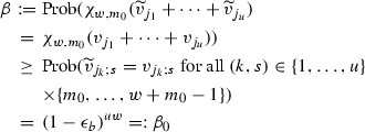  (17)

• (ii) [special case $u = 2$] For a randomly selected window pattern wp, we obtain the average probability

  $$\begin{aligned}&\overline{\beta }=\left( \begin{array}{cccc}1&0&0&0\end{array}\right) \nonumber \\&\quad \left( \begin{array}{llll} (1-\epsilon _b)^2&{}\quad \epsilon _b^2/4&{}\quad \epsilon _b^2/4&{}\quad 2\epsilon _b-\epsilon _b^2/2\\ \epsilon _b(1-\epsilon _b)&{}\quad \epsilon _b(1-\epsilon _b)&{}\quad 0&{}\quad 1-2\epsilon _b(1-\epsilon _b)\\ \epsilon _b(1-\epsilon _b)&{}\quad 0&{}\quad \epsilon _b(1-\epsilon _b)&{}\quad 1-2\epsilon _b(1-\epsilon _b)\\ 0&{}\quad 0&{}\quad 0&{}\quad 1 \end{array}\right) ^w\nonumber \\&\quad \times \left( \begin{array}{c}1\\ 1\\ 1\\ 0\end{array}\right) \,. \end{aligned}$$

  (18)

Proof

Formula (17) is obvious since the condition ${\widetilde{v}}_{j_k;s}= v_{j_k;s}$ for all $(k,s)\in \{1,\ldots ,u\}\times \{{m_{0}},\ldots ,w+{m_{0}}-1\}$ implies $\chi _{w,{m_{0}}}({\widetilde{v}}_{j_1}+\cdots +{\widetilde{v}}_{j_u})=\chi _{w,{m_{0}}}(v_{j_1}+\cdots +v_{j_u})$. Equation (17) follows from the assumed independence of the bit guesses. For the proof of (ii), we assume that ${\widetilde{v}}_{j_1}+{\widetilde{v}}_{j_2}$ is computed as in the schoolbook, bit by bit from the right to the left. Due to the pre-correction of the guesses ${\widetilde{v}}_{j_1}$ and ${\widetilde{v}}_{j_2}$ the lowest ${m_{0}}$ bits of their sum and the carry $\widetilde{ca}_{m_{0}}\in \{0,1\}$ are correct. At bit $s\in \{{m_{0}},\ldots ,w+{m_{0}}-1\}$ the addition operation is in one of four possible states $\varOmega :=\{0,+,-,\infty \}$. For the states $0,+,-$, the bits $s-1,\ldots ,0$ of the sum ${\widetilde{v}}_{j_1}+{\widetilde{v}}_{j_2}$ are correct, i.e. coincide with those of $v_{j_1}+v_{j_2}$. For state 0 (resp., for state $+$, resp., for state −) additionally $\widetilde{ca}_s=ca_s$ (resp., $\widetilde{ca}_s=ca_s+1$, resp., $\widetilde{ca}_s=ca_s-1$) holds. State $\infty$ (absorbing state) means that some bit $t\in \{0,\ldots ,s-1\}$ of ${\widetilde{v}}_{j_1}+{\widetilde{v}}_{j_2}$ is wrong, which excludes $\chi _{w,{m_{0}}}({\widetilde{v}}_{j_1}+{\widetilde{v}}_{j_2})=\chi _{w,{m_{0}}}(v_{j_1}+v_{j_2})$. Of course, $(v_{j_1;s},v_{j_2;s})\in \{(0,0),(0,1),(1,0),(1,1)\}$, and all four cases occur with probability 1 / 4. We exemplarily treat the conditional probability $\mathrm{Prob}(0\mid +)$ where ‘$+$’ means the state at bit s and ‘0’ the state at bit $s+1$. For $(v_{j_1;s},v_{j_2;s})=(0,0)$ this transition is impossible, for $(v_{j_1;s},v_{j_2;s})\in \{(0,1),(1,0)\}$ this transition occurs when $({\widetilde{v}}_{j_1;s},{\widetilde{v}}_{j_2;s})=(0,0)$ while finally $({\widetilde{v}}_{j_1;s},{\widetilde{v}}_{j_2;s})\in \{(0,1),(1,0)\}$ ensures this transition for $(v_{j_1;s},v_{j_2;s})=(1,1)$. The weighted sum of the four transition probabilities gives the conditional probability $\epsilon _b(1-\epsilon _b)$. The other transition probabilities can be treated likewise. The transition matrix in (18) can be expressed as $0.25(P_{00}+P_{01}+P_{10}+P_{11})$ where $P_{ik}$ denotes the transition matrix if $(v_{j_1;s},v_{j_2;s})=(i,k)$. Hence, (18) computes the average probability $\overline{\beta }$. $\square$

Remark 1

[Exact probabilities]

• (i) The Eq. (18) gives the (exact) average probability that the 2-sum of two guessed blinded exponents, ${\widetilde{v}}_{j_1}+{\widetilde{v}}_{j_2}$, has the same window pattern as the 2-sum of the true blinded exponents, $v_{j_1}+v_{j_2}$. In the proof of Lemma 3 it became clear that for a fixed word pattern wp the corresponding probability $\beta$ may differ from $\overline{\beta }$ since the values $\{(v_{j_1;s},v_{j_2;s})\mid {m_{0}}\le s \le w+{m_{0}}-1\}$ determine the sequence of transition matrices $P_{ik}$. For moderate parameters $(w,\epsilon _b)$, the relative difference $(\overline{\beta }-\beta _0)/\beta _0$ is small (c.f. Example 2). Anyway, $\overline{\beta }\ge \beta _0$.

• (ii) Of course, for $u>2$ pendants to (18) can be derived analogously. Then, $\varOmega =\{0,+_1,\ldots ,+_{u-1},-_1,\ldots ,-_{u-1},\infty \}$ where ‘$+_a$’ means $\widetilde{ca}_s=ca_s+a$, etc. As for $u=2$ one might assume that the relative difference between $\beta$ and its approximation $\beta _0$ is small.

Example 2

• (i) Let $(u,w,\epsilon _b)=(2,46,0.07)$. By (17) and (18) $\overline{\beta }=1.28\cdot 10^{-3}$, $\beta _0=1.26\cdot 10^{-3}$, and $\overline{\beta }/\beta _0=1.01$.

• (ii) Let $(u,w,\epsilon _b)=(2,46,0.10)$. Then $\overline{\beta }=6.4\cdot 10^{-5}$, $\beta _0=6.2\cdot 10^{-5}$, and $\overline{\beta }/\beta _0=1.04$.

If $(j_1,\ldots ,j_u)\sim (i_1,\ldots ,i_u)$ then in particular ${\chi }_{w,{m_{0}}}(v_{j_1}+\cdots +v_{j_u}) = {\chi }_{w,{m_{0}}}(v_{i_1} + \cdots + v_{i_u})$. The u-sums ${\widetilde{v}}_{j_1}+\cdots +{\widetilde{v}}_{j_u}$ and ${\widetilde{v}}_{i_1} + \cdots + {\widetilde{v}}_{i_u}$ are compared in Step (1d) iff the same window pattern is assigned to both u-sums. Lemma 3 considers the probability that all bit guesses within the window are correct and, more generally, that the window pattern for a u-tuple is correct. Of course, guessing errors in the summands of two u-sums might compensate one another, yielding false but identical guessed window patterns. Then, the enhanced plus attack would detect a linear equation anyhow. This would be the case, for instance, if $e_{j_1;s}=e_{i_u;s}=1$ for some $s\in \{m_0,m_0+1,\ldots ,m_0+w-1\}$ while all other bit guesses within the window are correct. Lemma 4 illuminates this scenario.

Lemma 4

Let $\{F_{j,i}\mid 1\le j \le 2u,\,0\le i\le w-1\}$ denote a family of iid random variables with $\mathrm{Prob}(F_{j,i}=0)=1-\epsilon _b$ and $\mathrm{Prob}(F_{j,i}=1)=\mathrm{Prob}(F_{j,i}=-1)=\epsilon _b/2$. Further, $G_j:=\sum _{i=0}^{w-1} F_{j,i} 2^i$ for $1\le j \le 2u$ and $H_i:=\sum _{j=1}^{2u} F_{j,i}$. Then

$$\begin{aligned}&\nu _H(x):=\mathrm{Prob}(H_i=x) \nonumber \\&\quad = {\mathop {\mathop {\sum }\limits _{0\le t \le 2u;}}\limits _{0\le v \le 2u-t; t-v = x}}{2u \atopwithdelims ()(2u-t-v),v}(1-\epsilon _b)^{2u-t-v} \left( \frac{\epsilon _b}{2}\right) ^{t+v}.\nonumber \\ \end{aligned}$$

(19)

for $x\in \{-2u,-2u+1,\ldots ,0,\ldots ,2u\}$ while $\nu _H(x)=0$ for $\vert x \vert >2u$. Let

(20)

If $j_1,\ldots ,j_u,i_1,\ldots ,i_u$ are mutually distinct

$$\begin{aligned} \mathrm{pr_{idpat}}:=\mathrm{Prob}\left( G_1+\cdots + G_{2u}\equiv 0 \bmod \,2^w\right) \,. \end{aligned}$$

(21)

Let $P=\left( p_{\omega _1,\omega _2}\right) _{\omega _1,\omega _2\in \varOmega }$ a transition matrix of a homogeneous Markov chain on the state space $\varOmega =\{0,1,\ldots ,2u,\infty \}$ where $\infty$ denotes an absorbing state. In particular, $p_{a,b}=\nu _H(2b-a)+\nu _H(-2b-a)$ for $a\in \{0,\ldots ,2u\}$ and $b\in \{1,\ldots ,2u\}$. For $a\in \{0,\ldots ,2u\}$ further $p_{a,0}=\nu _H(a)$, $p_{a,\infty }=\sum _{x\equiv a+1\bmod \,2}\nu _H(x)$, $p_{\infty ,a}=0$ and $p_{\infty ,\infty }=1$. If $j_1,\ldots ,j_u,i_1,\ldots ,i_u$ are mutually distinct then

$$\begin{aligned} \mathrm{pr_{idpat}}=(1,0\ldots ,0) P^w \left( \begin{array}{c}1\\ 1\\ \vdots \\ 1\\ 0\end{array}\right) \end{aligned}$$

(22)

Proof

Formula (19) is obvious. Due to the pre-correction step from Sect. 3.2 we may assume $e_{s;i}=0$ for $s\in \{j_1,\ldots ,j_u,i_1,\ldots ,i_u\}$ and $i=0,\ldots ,m_0-1$. Hence ${\chi }_{w,{m_{0}}}({\widetilde{v}}_{j_1}+\cdots +{\widetilde{v}}_{j_u})={\chi }_{w,{m_{0}}}({\widetilde{v}}_{i_1}+\cdots +{\widetilde{v}}_{i_u})$ iff

$$\begin{aligned}&v_{j_1}+e_{j_1}+\cdots +v_{j_u}+e_{j_u}-\left( v_{i_1}+e_{i_1}+\cdots +v_{i_u}+e_{i_u}\right) \\&e_{j_1}+\cdots +e_{j_u}-\left( e_{i_1}+\cdots +e_{i_u}\right) \equiv 0 \bmod \,2^{m_0+w}. \end{aligned}$$

Since the blinding factors $r_{j_1},\ldots ,r_{i_u}$ were selected randomly we may assume that the bits $v_{s,m_0},\ldots ,v_{s,m_0+w-1}$ are realizations of iid uniformly distributed $\{0,1\}$-valued random variables. Consequently, $e_{s;m+i}$ be interpreted as a realization of the random variable $F_{s,i}$. Hence $\mathrm{pr_{idpat}}=\mathrm{Prob}(G_1+\cdots +G_u-G_{u+1}-\cdots - G_{2u}\equiv 0 \bmod \,2^{w})$. Since the random variables $F_{j,i}$ are symmetrically distributed with regard to 0 this is also valid for the random variables $G_j$ and $H_i$, which proves (21).

Table 2 Several ratios $\mathrm{pr_{idpat}}/\beta _0^{2}$ for exemplary parameter sets under the condition that $j_1,\ldots ,j_u,i_1,\ldots ,i_u$ are mutually distinct. The ratio increases when the window size w or the error rate $\epsilon _b$ increase

Now $G_1+\cdots G_{2u} = \sum _{i=0}^{w-1} H_i 2^i \equiv 0 \bmod \,2^w$ iff $\sum _{i=0}^{s} H_i 2^i \equiv 0 \bmod \,2^{s+1}$ for $s=0,\ldots ,w-1$. The second condition is equivalent to $(H_s+ca_s)2^s \equiv 0 \bmod \,2^{s+1}$ (resp., to $H_s+ca_s \equiv 0 \bmod \,2$) for $s=0,\ldots ,w-1$ with $ca_s=\left\lfloor \sum _{i=0}^{s-1} H_i 2^i/2^{s}\right\rfloor$. Further, $ca_{s+1}=\lfloor (ca_{s}+H_{s})/2\rfloor$. By induction, $\vert ca_s\vert \le 2u$. We may interpret the values $ca_0,ca_1,\ldots ,ca_w$ as realizations of a finite Markov chain on the state space $\varOmega ':=\{-2u,-2u+1,\ldots ,2u-1,2u,\infty \}$ with transition matrix $P'=(p'_{\omega '_1,\omega '_2})_{\omega '_1,\omega '_2\in \varOmega '}$. In particular, $\infty$ is an absorbing state, which is reached when $ca_s+H_s\equiv 1 \bmod \,2$ for some $s\in \{0,\ldots ,w-1\}$. (Then $ca_{s+1},\ldots ,ca_{w}$ do not represent carry values but assume the value $\infty$.) Further, $p_{a,b}:=\nu _H(2b-a)$ for $-2u\le a,b \le 2u$ since a transition from state a to state b occurs iff $a+H_s=2b$. Finally, $p_{a,\infty }=\sum _{x\equiv a+1\bmod \,2}\nu _H(x)$.

Consider the partition $\{-2u,2u\},\{-2u+1,2u-1\},\ldots ,\{1,-1\},\{0\},\{\infty \}$ of $\varOmega '$: Since the random variables $H_i$ are symmetrically distributed with regard to 0 we conclude that $p_{a,b}+p_{a,-b}=p_{-a,b}+p_{-a,-b}$ for $a,b\not \in \{0,\infty \}$. Further, $p_{a,0}=p_{-a,0}$ and $p_{a,\infty }=p_{-a,\infty }$ for $a\not =\infty$ since $a+x\equiv -a+x \bmod \,2$. Thus, the Markov chain on $\varOmega '$ is lumpable with regard to this partition, see [5], Definition 6.3.1 and Theorem 6.3.2. This means that the stochastic process on this partition, which is induced by the mapping $a\mapsto \{-a,a\}$ for $a\notin \{0,\infty \}$ and $0\mapsto \{0\}$ and $\infty \mapsto \{\infty \}$ is itself Markovian. If we identify $\{a,-a\}$ with a, $\{0\}$ with 0 and $\{\infty \}$ with $\infty$ this yields the Markov chain on the state space $\varOmega$, which is defined after (21). Formula (22) finally follows from the fact that $G_1+\cdots G_{2u} \not \equiv 0 \bmod \,2^w$ iff the Markov chain assumes the absorbing state $\infty$ after w steps. $\square$

While the relative difference between the probability $\beta$ and its approximation $\beta _0$ usually is small (c.f. Remark 1) the relative difference between $\mathrm{pr_{idpat}}$ and $\beta _0^2$ usually is not and thus has significant impact on the estimated overall workload of the attack. In particular, one should not proceed with $\beta _0^2$ in place of $\mathrm{pr_{idpat}}$ although it is easy to calulate. Table 2 contains figures for some parameter vectors $(\epsilon _b,w,u)$. Recall that the term $\beta _0^{2}$ equals the probability that $e_{s;i}=0$ for $s\in \{j_1,\ldots ,j_u,i_1,\ldots ,i_u\}$ and $i\in \{m_0,\ldots ,m_0+w-1\}$.

Lemma 5 quantifies the minimum value for the sample size N, which is needed to obtain sufficiently many linear equations.

Lemma 5

Assume that $u\ll N$ while $\alpha$ and $\mathrm{pr_{idpat}}$ are defined as in Lemma 1 and in Lemma 4, respectively. In particular, the probability $\mathrm{pr_{idpat}}$ is given by (22).

• (i) For sample size, N, we expect

  $$\begin{aligned} \mathrm{E}(\#\hbox {linear equations}) \approx \frac{N^{2u}}{2u!u!}\frac{c(u)\alpha \mathrm{pr_{idpat}}}{2^R}\,. \end{aligned}$$

  (23)

• (ii) To get 2N linear equations in average, one needs $N\ge N_2$ power traces with

  $$\begin{aligned}&N_2= \left( \frac{u!u!2^{R+2}}{c(u)}\cdot \frac{1}{\alpha \mathrm{pr_{idpat}}}\right) ^{\frac{1}{2\cdot u-1}}\,.\nonumber \\&\quad \hbox {The array { L} then contains} \end{aligned}$$

  (24)
  $$\begin{aligned}&\quad \approx \frac{N_2^u}{u!}=\left( \frac{u!u!2^{R+2}}{c(u)}\cdot \frac{1}{\alpha \mathrm{pr_{idpat}}}\right) ^{\frac{u}{2\cdot u-1}}\frac{1}{u!}\nonumber \\&\quad \hbox {table entries.} \end{aligned}$$

  (25)
  $$\begin{aligned}&\hbox {This costs }\approx \left( \frac{u!u!2^{R+2}}{c(u)}\cdot \frac{1}{\alpha \mathrm{pr_{idpat}}}\right) ^{\frac{2u}{2\cdot u-1}}\frac{2^{-(w+1)}}{u!u!}\nonumber \\&\quad \hbox { NAF calculations.} \end{aligned}$$

  (26)

Proof

Formula (26) in [8] says that for N power traces one may expect that the enhanced attack detects $\approx \alpha (N^{2u}c(u))/(2u!u!2^R)$ linear equations. For a realistic parameter N the condition ’$j_1,\ldots ,j_u,i_1,\ldots ,i_u$ are mutually distinct’ should be fulfiled for almost all of these equations. Hence, we may expect that in Step (1d) of the enhanced plus attack a fraction of $\approx \mathrm{pr_{idpat}}$ of these linear equations are detected, where $\mathrm{pr_{idpat}}$ is given by (22), which verifies (23). Solving the equation $2N\le N^{2u}c(u)\mathrm{pr_{idpat}}\alpha / (2u!u! 2^R)$ yields (24) while (25) and (26) are immediate consequences of (24), (9) and Lemma 2. $\square$

Assume for the moment that the parameters $k,R,\epsilon _b,b_0$ are fixed. Since $\mathrm{pr_{idpat}}$ is a function of $\epsilon ,w$ and u we write $\mathrm{pr_{idpat}}(\epsilon ,w,u)$ for the moment. For window size, w (9) and (24) imply that the array L contains $const_L\cdot (1/\mathrm{pr_{idpat}}(\epsilon _b,w,u))^{2u/(2u-1)}$ elements in average. Similarly, (26) the expected number of $\mathrm{NAF}$ calculations is $const_N \cdot (1/\mathrm{pr_{idpat}}(\epsilon _b,w,u))^{2u/(2u-1)}2^{-w}$. It is natural to ask where the limits of the enhanced plus attack are and whether it is superior to the enhanced attack for each error rate $\epsilon _b$ since more and more equations get lost in Step (1d) when $\epsilon _b$ increases.

Due to (22) we may assume that the term $\mathrm{pr_{idpat}}^{1/w}(\epsilon _b,w,u)$ converges rapidly to some limit $\rho (\epsilon _b,u)$ as w increases (mainly driven by the second largest eigenvalue of P). Of course, if $2^{(2u-1)/2u}\rho (\epsilon _b,u)<1$ increasing the window size w increases the number of NAF calculations. This boundary value for $\epsilon _b$ constitutes an upper bound for the limits of the enhanced plus method because the best an attacker then can do is to select a small window size w. Numerical experiments show that the critical values for $\epsilon _b$ are $\approx 0.15$ (for $u=2$), 0.125 (for $u=3$) and 0.105 (for $u=4$), respectively. It should be noted that the enhanced plus attack requires more power traces than the enhanced attack and, in particular, much more memory and sorting operations are necessary. Table 3 shows that the enhanced plus attack is usually superior to the enhanced attack while $(k,R,\epsilon _b) = (1024,32,0.14)$ is an exception.

Table 3 Enhanced plus attack versus enhanced attack: figures for exemplary parameter sets

3.5 Attack efficiency (Step 1)

In this subsection, we compare Step 1 of the enhanced attack with Step 1 of the enhanced plus attack. The Substeps (1b), (1c) and in particular (1d) the enhanced plus attack determine the non-experimental workload. Table 3 contains figures for many parameter sets. The term $\vert L \vert$ denotes the number of elements of the array L. The storage size for L depends on the type of the data sets, c.f. (10), (11), (12). For Table 3 we applied (4), (5), (24), (25) and (26). As in [8], we estimated $\mu _{W'}$ and $\sigma _{W'}$ experimentally on basis of numerical simulation experiments. We express the decision boundary in the form $b_0=\mu _W-c_0\sigma _W$. The expected number of false positives (erroneously collected false linear equations) is $\approx \varPhi (-c_0)\cdot \# \{\mathrm{NAF}$ operations$\}$, while $\alpha =\varPhi ((b_0-\mu _{W'})/\sigma _{W'})$ quantifies the fraction of detected correct equations. Since false positives need to be detected and removed for attack step 2 [8, Sect. 3.3.3] for Table 3 we selected factors $c_0$ such that the expected number of false positives is smaller than 1, for most of the parameter sets it is even significantly below 1. For fixed (k, R, u) the sample size, the memory and the number of NAF computations increase when the error rate $\epsilon _b$ increases. This is due to the fact that the ratio $\alpha$ of detected linear equations decreases, which limits the tolerable error rate. Hence, one may assume that in Table 3 the results for large error rates are more sensitive to statistical deviations of the estimates for $\mu _{W'}$ and $\sigma _{W'}$ than for small $\epsilon _b$.

Depending on (k, R, u), there exists a threshold $\hbox {eps}$ such that $\alpha \approx 1$ for all $\epsilon _b\le \hbox {eps}$. Formulae (4) and (5) imply that the workload of the enhanced attack is essentially the same for all these $\epsilon _b$ and increases when $\epsilon _b$ exceeds $\hbox {eps}$. For $(k,R,u)=(1024,32,2)$ figures from Table 3 verify this property experimentally.

In contrast, the enhanced plus attack is very sensitive against changes of $\epsilon _b$. As the error rate increases, the fraction of linear equations decreases, which are detected in Substep (1d). This phenomenon is quantified by the probability $\mathrm{pr_{idpat}}$. The enhanced plus attack is superior to the enhanced attack for most of the error rates $\epsilon _b$ but may be inferior for large $\epsilon _b$. This is certainly the case for $(k,R,\epsilon _b)=(1024,32,0.14)$. The choice of a suitable window size w is a trade-off between the sample size, the memory size and the computational workload.

An important question clearly is for which parameter sets the enhanced attack and the enhanced plus attack are practical. In the very end this means that one has to decide whether a (powerful) attacker is able (or maybe more precisely: whether he is willing) to spend sufficient resources to perform a particular attack. It is hardly possible to define a clearcut boundary between practicability and impracticability. In our opinion by all necessary caution $\log _2(\vert L\vert )\le 60$ is a reasonable threshold for the number of elements in the array L since this requires $\approx 2^{24}$ TB memory (for short data records) or even $\approx 2^{27}$ TB memory (for full data records), which is gigantic. For the average number of NAF Hamming weight computations, a threshold between $2^{70}$ and $2^{75}$ seems to be reasonable due to the general uncertainties of a side-channel attack, here especially due to the variance of the number of computations and possible deviations from the estimated error probability $\epsilon _b$, which would also affect the number of NAF Hammning weight computations.

In Sect. 5, we compare the efficiency of the enhanced attack, the enhanced plus attack and the alternate attack, which is analysed in Sect. 4.

4 Alternate attack on RSA with CRT

In [8, Sect. 4.2], the so-called alternate attack on RSA without CRT was introduced. In the first attack step, blinding factors are guessed, and in the second step $y=\phi (n)$ is recovered with the error detection and correction Algorithm 2 in [8], which coincides with Step 3 of the enhanced attack. The first attack step exploits the fact that the upper halve of the bits of $y=\phi (n)\approx n$ is known, which is not the case for RSA with CRT.

In this section, we introduce an algorithm (continued fraction method), which allows to recover the most significant 2R bits of $y=\phi (p)$ for RSA with CRT. After this pre-step, the above-mentioned alternate attack can be applied to RSA with CRT, too (although only the $\approx 2R$ most significant bits of y are known here).

Section 4.1 explains the basic idea of the continued fraction attack method, and Sect. 4.2 formulates the continued fraction algorithm. Justifications of this algorithm and explanations, efficiency considerations and simulation results follow in the subsequent subsections. Finally, Sect. 4.5 reconsiders the alternate attack from [8, Sect. 4.2], which constitutes the second attack step in our case.

4.1 Basic idea

Recall that d and y are unknown. We consider the three equations

$$\begin{aligned} v_1=r_1y +d,\qquad v_2=r_2y +d,\qquad v_3=r_3y +d\,. \end{aligned}$$

(27)

with $0\le r_1,r_2,r_3 < 2^R$ and $2^{k-1} \le y < 2^k$. The attacker only knows guesses $\widetilde{v}_1, \widetilde{v}_2,\widetilde{v}_3$ of the blinded exponents $v_1,v_2,v_3$, If he knew the correct values $v_1,v_2,v_3$ recovering y would be rather simple since $y | \mathrm{GCD}(\vert v_1-v_2\vert ,\vert v_1-v_3\vert )$. For simplicity, we assume that $\mathrm{GCD}(\vert r_1-r_2\vert ,\vert r_1-r_3\vert ) =1$, which implies

$$\begin{aligned} y = \mathrm{GCD}(\vert v_1-v_2\vert ,\vert v_1-v_3\vert )\,. \end{aligned}$$

(28)

(Remark 4 discusses the case ’${>}1$’.) Then y can be computed with the well-known Euclidean algorithm. Some basic observations:

• 1. Usually, the first steps of the computation of $\mathrm{GCD}(\vert v_1-v_2\vert ,\vert v_1-v_3\vert )$ should only depend on the most significant bits of the values $\vert v_1-v_2\vert$ and $\vert v_1-v_3\vert$.

• 2. The $\mathrm{GCD}$-computation stops when the remainder 0 occurs. The extended Euclidean algorithm yields a representation

  $$\begin{aligned}&\lambda _1 (v_1-v_2) + \lambda _2 (v_1-v_3) =0\nonumber \\&\qquad \hbox {with } \lambda _1 =\pm (r_1-r_3) \hbox { and } \lambda _2 =\pm (r_1-r_2)\,. \end{aligned}$$

  (29)

• 3. Finally, y can be computed by

  $$\begin{aligned} y= \left| \frac{v_1-v_3}{r_1-r_3} \right| = \left| \frac{v_1-v_3}{\lambda _1} \right| \,. \end{aligned}$$

  (30)

4.2 Recovering the most significant bits of y

In this section, we formulate the main algorithm, which applies continued fraction expansion. For the moment, we fix the integers N, s and $m_0$.

Algorithm 1

Continued fraction attack (aims at the most significant bits of $y = \phi (p)$)

• 1. Set $S=\{ \}$.

  • (a) Choose a new triple of three ordered indices $1\le j_1< j_2 < j_3 \le N$, which is different to the choices before.

  • (b) Generate all triples $(v^*_{j_1}, v^*_{j_2},v^*_{j_3})$, which differ in each component in at most $m_0$ bits from $(\tilde{v}_{j_1}, \tilde{v}_{j_2},\tilde{v}_{j_3})$ within the most significant bits beginning with position s.

  • (c) Compute the continued fraction expansion $(\frac{p_{\mu }}{q_{\mu }})_{\mu }$ of the rational quotient

    $$\begin{aligned} \left| \frac{v^*_{j_1}-v^*_{j_2}}{v^*_{j_1}-v^*_{j_3}} \right| \end{aligned}$$

    (31)

    Take the best approximation $\mu _0=p_{\mu _0}/q_{\mu _0}$, i.e. which minimizes the difference

    $$\begin{aligned} \left| \left| \frac{v^*_{j_1}-v^*_{j_2}}{v^*_{j_1}-v^*_{j_3}} \right| - \frac{p_{\mu }}{q_{\mu }} \right| \end{aligned}$$

    (32)

    subject to the conditions $p_{\mu } \le 2^R$ and ${q_{\mu }} \le 2^R$.

  • (d) For this approximation, calculate

    $$\begin{aligned} x_q:= \left\lfloor \left| \frac{ v^*_{j_1}-v^*_{j_3} }{ q_{\mu _0} } \right| \right\rfloor \quad \hbox {and}\quad x_p:= \left\lfloor \left| \frac{ v^*_{j_1}-v^*_{j_2} }{ p_{\mu _0} } \right| \right\rfloor \,. \end{aligned}$$

    (33)

    If $q_{\mu _0} \ge p_{\mu _0}$, set $x:= x_q$, else set $x:= x_p$. Set $S :=S \cup \{ x \}$, if $2^{k-1}< x < 2^k$.

• 2. Identify clusters within the set S. The most significant bits of their elements are the candidates for the most significant bits of y (c.f. Sect. 4.3 for details).

4.3 Justification and explanations

In this subsection, we motivate Algorithm 1 and illuminate its background. For basic facts and properties of continued fractions, we refer the interested reader, e.g. to [4], Chapter X.

Remark 2

[Memory and sorting operations]

• (i) Since the numbers $p_{\mu }$ and $q_{\mu }$ increase during the continued fraction expansion Step 1(c) of Algorithm 1 can be computed efficiently.

• (ii) Algorithm 1 stores $N'$ data sets of the form

  $$\begin{aligned}&j_1 || j_2 || j_3 || x \qquad \hbox {(full data record)}\nonumber \\&\hbox {storage space: } \ge (4\cdot 3 + \lceil k/8 \rceil )\qquad \hbox {bytes}\,. \end{aligned}$$

  (34)

  The memory per data set is nearly the same as for (10). In order to save memory, the component x might be replaced by (e.g.) its 3R most significant bits (c.f. Remark 6(ii)). In this case, the memory per data set drops down to $\approx 4\cdot 3 + \lceil 3R/8 \rceil$ bytes.

• (iii) In Step 2 of Algorithm 1 the set S contains $N'$ elements (with $N'$ = # of continued fraction expansions), which have to be sorted with regard to their last components. The situation is less comfortable than for the enhanced plus attack since S must be totally sorted, and it is not clear whether the elements of S are (at least nearly) uniformly distributed on their range. Similarly as in Sect. 3.3 one may try to reduce the number of sorting operations below $O(N'\log (N'))$, which is needed by the Quicksort algorithm (with some small constant in the average case). On basis of the $w'$ most significant bits of x one may assign a data set $(j_1,j_2,j_3,x)$ directly to one of $2^{w'}$ subarrays. If these subarrays are sorted with the Quicksort algorithm in the best case $O(N'\log (N'2^{-w'}))$ operations are needed. If the sizes of these $2^{w'}$ subarrays are very different the sorting workload will be larger. (Our experiments did not show indicators therefor.) Moreover, as in Sect. 3.3 one might to try to put each tuple $(j_1,j_2,j_3,x)$ close to its final position within the subarray. Altogether, the overall number of sorting operations should be somewhere between $O(N')$ and $O(N'\log (N'))$.

Algorithm 1 can only be successful if certain conditions are met. In the following, we will discuss the situation. Let $\zeta > 0$ be a real number, A and B positive integers with $\mathrm{GCD}(A,B) =1$. If the approximation A / B occurs within the continued fraction expansion of $\zeta$, i.e.

$$\begin{aligned} \hbox {if }\frac{A}{B} = \frac{p_\mu }{q_\mu }\quad \hbox { for a suitable index }\mu \quad \hbox { then } B \vert B\zeta -A \vert \le 1 \end{aligned}$$

(35)

by [4], Theorem 163. On the other hand, in a certain sense [4], Theorem 184, guarantees the converse:

$$\begin{aligned}&\hbox {If }B \vert B\zeta -A \vert \le \frac{1}{2}\qquad \hbox { then }\nonumber \\&\frac{A}{B}\hbox { can be computed by the continued fraction expansion of }\zeta .\nonumber \\ \end{aligned}$$

(36)

If the values $v_1^*$, $v_2^*$ and $v_3^*$ in Step 1 of Algorithm 1 are correct at the bit positions $k+R-1, \ldots ,s$ (i.e. in the $(k+R-s)$ most significant bits) then

$$\begin{aligned}&\vert v^*_{j_1}-v^*_{j_2} \vert = \vert r_{j_1}-r_{j_2} \vert y + \delta _1 \quad \hbox { and }\nonumber \\&\vert v^*_{j_1}-v^*_{j_3} \vert = \vert r_{j_1}-r_{j_3} \vert y + \delta _2\hbox { with }\vert \delta _j\vert \approx 2^s\,. \end{aligned}$$

(37)

This gives

$$\begin{aligned}&\frac{|v^*_{j_1}-v^*_{j_2} |}{|r_{j_1}-r_{j_2} |} = y + \frac{\delta _1}{|r_{j_1}-r_{j_2} |}\quad \hbox {and}\nonumber \\&\frac{|v^*_{j_1}-v^*_{j_3} |}{|r_{j_1}-r_{j_3} |} = y + \frac{\delta _2}{|r_{j_1}-r_{j_3} |}\nonumber \\&\qquad \hbox {with}\,\frac{\delta _1}{|r_{j_1}-r_{j_2} |},\frac{\delta _2}{|r_{j_1}-r_{j_3} |}\approx 2^{s-R} \end{aligned}$$

(38)

This observation motivates Step 1(d) of Algorithm 1. In order to minimize the deviation to y, we always decide for the larger of the two values $|r_{j_1}-r_{j_2} |$ and $|r_{j_1}-r_{j_3} |$. Multiplying the equations in (37) by $\vert r_{j_1}-r_{j_3} \vert$ and by $\vert r_{j_1}-r_{j_2} \vert$, respectively, and subtracting the second from the first leads to

$$\begin{aligned}&\left| \vert r_{j_1}-r_{j_3} \vert \cdot \vert v^*_{j_1}-v^*_{j_2} \vert - \vert r_{j_1}-r_{j_2} | \cdot \vert v^*_{j_1}-v^*_{j_3} \vert \right| \nonumber \\&\quad = \left| \vert r_{j_1}-r_{j_3} \vert \cdot \delta _1 - |r_{j_1}-r_{j_2} \right| \cdot \delta _2 | \approx 2^{s+R} \end{aligned}$$

(39)

If additionly $\mathrm{GCD}(\vert r_{j_1}-r_{j_2}\vert ,\vert r_{j_1}-r_{j_3}\vert ) =1$ we may expect that the set S contains a good approximation of y as long as $s \le k-R$. In fact, as already deduced in (38) $\vert (v^*_{j_1}-v^*_{j_3})/(r_{j_1}-r_{j_3})-y\vert = \vert \delta _2\vert /(r_{j_1}-r_{j_3})\approx 2^{s-R}$. This is roughly the bound of [4], Theorem 184. We set $s=k-R$ in the following. Due to (38), we may expect to learn the $\approx 2R$ most significant bits of y from Algorithm 1.

We set

$$\begin{aligned} f:= \left| \frac{ \vert r_{j_1}-r_{j_3} \vert \delta _1 - \vert r_{j_1}-r_{j_2} \vert \delta _2 }{ y + \delta _2/ \vert r_{j_1}-r_{j_3}\vert }\right| \end{aligned}$$

(40)

We demand $f \le 1/2$. By (36) then (with $\zeta = \vert v^*_{j_1}-v^*_{j_2} \vert / \vert v^*_{j_1}-v^*_{j_3} \vert$, $A=\vert r_{j_1}-r_{j_2} \vert$ and $B= \vert r_{j_1}-r_{j_3} \vert$) we know that the correct values $\vert r_{j_1}-r_{j_2} \vert , \vert r_{j_1}-r_{j_3}\vert$ will occur within the continued fraction expansion of $\zeta$ provided that $\mathrm{GCD}(\vert r_{j_1}-r_{j_2}\vert ,\vert r_{j_1}-r_{j_3}\vert ) =1$. However, it is not true that this fraction is automatically the best approximation in Step 1(c) of Algorithm 1.

Remark 3

By looking deeper into the computation of the continued fraction expansion, we can illustrate this effect: During the computation, the approximations ${p_\mu }/{q_\mu }$ are given as a $2\times 2$-matrix

$$\begin{aligned} \begin{pmatrix} p_\mu &{}\quad p_{\mu -1} \\ q_\mu &{}\quad q_{\mu -1} \end{pmatrix} \end{aligned}$$

(41)

A basic property of the continued fraction algorithm is that the inverse of this matrix multiplied by the vector $(\vert v^*_{j_1}-v^*_{j_2}\vert ,\vert v^*_{j_1}-v^*_{j_3}\vert )^T$ just gives the intermediate values of the GCD-computation. If the correct approximation is computed in step $\mu$, the corresponding matrix is

$$\begin{aligned} \begin{pmatrix} \vert r_{j_1}-r_{j_2} \vert &{} E_1 \\ \vert r_{j_1}-r_{j_3} \vert &{} E_2 \end{pmatrix} \end{aligned}$$

where $(E_1,E_2)$ is exactly one of the pairs of Bezout’s identity:

$$\begin{aligned} \vert r_{j_1}-r_{j_2} \vert \cdot E_2 - \vert r_{j_1}-r_{j_3} \vert \cdot E_1 = \pm 1 \end{aligned}$$

with $0< E_1 < \vert r_{j_1}-r_{j_2} \vert$ and $0< E_2 < \vert r_{j_1}-r_{j_3} \vert$. The intermediate values of the GCD-computation in step $\mu$ are given by

$$\begin{aligned} \begin{pmatrix} \vert r_{j_1}-r_{j_2} \vert &{} E_1 \\ \vert r_{j_1}-r_{j_3} \vert &{} E_2\\ \end{pmatrix}^{-1} \begin{pmatrix} \vert v^*_{j_1}-v^*_{j_2}\vert \\ \vert v^*_{j_1}-v^*_{j_3}\vert \, \end{pmatrix}. \end{aligned}$$

which gives the intermediate values

$$\begin{aligned} y \pm (E_2\delta _1-E_1\delta _2) \hbox { and } f \cdot ( y + \delta _2/ \vert r_{j_1}-r_{j_3} \vert ) \end{aligned}$$

Therefore, the subsequent GCD-step is of the form

$$\begin{aligned} y \pm (E_2\delta _1-E_1\delta _2)= & {} F \cdot f \cdot ( y + \delta _2/ \vert r_{j_1}-r_{j_3} \vert )\\&+ \hbox { remainder } \end{aligned}$$

The left side of this equation is in the range of y, so that F is in the range of 1 / f. The next approximation is given by

$$\begin{aligned} \begin{pmatrix} \vert r_{j_1}-r_{j_2} \vert &{} E_1 \\ \vert r_{j_1}-r_{j_3} \vert &{} E_2 \end{pmatrix} \begin{pmatrix} F &{} 1 \\ 1 &{} 0 \end{pmatrix} = \begin{pmatrix} \vert r_{j_1}-r_{j_2} \vert \cdot F +E_1 &{} \vert r_{j_1}-r_{j_2} \vert \\ \vert r_{j_1}-r_{j_3} \vert \cdot F +E_2 &{}\vert r_{j_1}-r_{j_3} \vert \end{pmatrix} \end{aligned}$$

If the entries of the left column of this matrix are both $\le 2^R$ then Algorithm 1 will not output the correct values for $r_{j_1}-r_{j_2}$ and $r_{j_1}-r_{j_3}$. In fact, the candidate x as computed in Step (1d) of Algorithm 1 will - very likely - not fulfil the condition $2^{k-1}< x < 2^k$. The probability of this event depends mainly on the size of F and $\vert r_{j_1}-r_{j_2} \vert$, $\vert r_{j_1}-r_{j_3} \vert$. In particular, if $\vert r_{j_1}-r_{j_2} \vert$ or $\vert r_{j_1}-r_{j_3} \vert$ are near to $2^R$ or f is small, the success rate of Algorithm 1 is very good.

With the same arguments as above we derive an approximation of y in the GCD-computation in the form of $y \pm (E_2\delta _1-E_1\delta _2)$. Note that this approximation is in general much worse than computing the quotient

$$\begin{aligned} \left| \frac{ v^*_{j_1}-v^*_{j_3} }{ q_{\mu _0} } \right| \end{aligned}$$

(42)

in Step 1(d) of Algorithm 1. We know that $y \pm (E_2\delta _1-E_1\delta _2)$ lies in the range of y. But we can quantify this approximation further in dependence of f: Note that

$$\begin{aligned} E_2\delta _1-E_1\delta _2 = \det \begin{pmatrix} \delta _1 &{} E_1 \\ \delta _2 &{} E_2 \end{pmatrix} \end{aligned}$$

The absolute value of the determinant of a $2\times 2$-matrix is the area of the parallelogram spanned by the columns of the matrix. Therefore, we have

$$\begin{aligned} \vert \det ( v&w ) \vert = \Vert v \Vert \cdot \Vert w \Vert \cdot \vert \sin (\alpha _{v,w}) \vert \end{aligned}$$

where $\alpha _{v,w}$ is the angle between the 2-dimensional vectors v and w. Using the elementary inequality $\vert \sin (\alpha +\beta )\vert \le \vert \sin (\alpha )\vert +\vert \sin (\beta )\vert$, we can easily derive the upper bound

$$\begin{aligned} \vert E_2\delta _1-E_1\delta _2 \vert\le & {} f \cdot (y + \delta _2/ \vert r_{j_1}-r_{j_3}\vert ) \\&+ \sqrt{\frac{ \delta _1^2+ \delta _2^2}{(r_{j_1}-r_{j_2})^2+ (r_{j_1}-r_{j_3})^2 } } \end{aligned}$$

The last formula suggests that the relative difference of $y \pm (E_2\delta _1-E_1\delta _2)$ to y mainly depends on f.

Remark 4

[$\hbox {GCD}>1$] Algorithm 1 may be adjusted that it also covers the case $\mathrm{GCD}(\vert r_{j_1}-r_{j_2}\vert ,\vert r_{j_1}-r_{j_3}\vert ) =\lambda > 1$. As long as $\lambda p_{\mu _0} \le 2^R$ and $\lambda {q_{\mu _0}} \le 2^R$ in Step 1(d) of Algorithm 1 we compute the value (if $q_{\mu _0} \ge p_{\mu _0}$)

$$\begin{aligned} x_q= \left\lfloor \left| \frac{ v^*_{j_1}-v^*_{j_3} }{ \lambda q_{\mu _0} } \right| \right\rfloor \,. \end{aligned}$$

(43)

If $2^{k-1}< x_q < 2^k$ then $S :=S \cup \{ x_q \}$. To prevent that the set S becomes too large we restrict ourselves to small factors, e.g. $\lambda \le 5$.

Remark 5

[Valuation of clusters] We need a suitable valuation method to detect and evaluate clusters in S (Step 2 of Algorithm 1). As an ad hoc approach we could simply count multiple occurrences of the roughly 2R most significant bits of our candidates x in S. In our experiments, we actually used another valuation function for the following reason: Let $R_1,R_2,R_3,\varDelta _1,\varDelta _2,\varDelta _3$ denote three independent random variables that are uniformly distributed on the interval [0, 1]. We define the random variable Z by

$$\begin{aligned} Z = \left\{ \begin{array}{ll} \frac{|\varDelta _3 -\varDelta _1|}{|R_3-R_1|} &{} \hbox { if } |R_3-R_1| > |R_2-R_1| \\ \frac{|\varDelta _2 -\varDelta _1|}{|R_2-R_1|} &{} \hbox { else. } \\ \end{array} \right. \end{aligned}$$

(44)

We computed the probability density function $f_Z(\tau )$ of Z as

$$\begin{aligned} f_Z(\tau )=\left\{ \begin{array}{ll} \frac{11}{12} -\frac{31\tau }{60} &{}\hbox { if } \tau< 1\\ -\frac{1}{12} +\frac{\tau }{60}+\frac{2}{3 \tau ^2} -\frac{1}{5 \tau ^4} &{}\hbox { if } 1 \le \tau < 2\\ \frac{4}{3\tau ^3} -\frac{1}{\tau ^4} &{}\hbox { if } 2 \le \tau \,. \end{array} \right. \end{aligned}$$

(45)

This formula requires elementary but long and careful calculations. To save space we omit the details. We assume that the elements of S are sorted in increasing order. For each $x_i$ in S, we compute its valuation

$$\begin{aligned} \hbox {Val}(x_i)=\sum _{j\ne i, |i-j| \le k_0} f_Z\left( \left| \frac{x_i-x_j}{2^{k-2R}}\right| \right) \,, \end{aligned}$$

(46)

and we select that $x_i$ as a candidate for y with the largest $\hbox {Val}(x_i)$. In the sum, we restrict ourselves to the $k_0$ nearest neighbours of $x_i$ from below and the $k_0$ nearest neightbours from above within the ordered set S. The threshold $k_0$ should be selected with regard to the number of expected good approximations of y. We mention that the maximum valuation can be computed efficiently by defining a suitable threshold value and applying an ‘early abort’ strategy.

Note: If we consider differences of neighboured candidates $x_{i+1}-x_i$ as independent random variables, one is let to replace the sum in $\hbox {Val}(x_i)$ by a product, e.g. by $\prod _{j, i+1\le j \le i+k_0} f_Z(|\frac{x_j-x_{j-1}}{2^{k-2R}}|)$ for all i and all small $k_0$. Since this product is very sensitive to the choice of the parameter $k_0$ we decided for the more robust valuation function (46).

4.4 Choice of the parameters, workload and simulation results

In this subsection, we discuss the choice of $m_0$ and N for Algorithm 1, its workload and success rates. We provide figures for many parameter sets and give simulation results.

The term

$$\begin{aligned} p_{m_0}:= \sum _{m\le m_0} {2R \atopwithdelims ()m} \epsilon _b^m (1-\epsilon _b)^{2R-m} \end{aligned}$$

(47)

quantifies the probability that at most $m_0$ guessing errors occur in the 2R most significant bits of a $\tilde{v}_{j}$. Moreover, we set

$$\begin{aligned} M_0:= \sum _{m\le m_0} {2R \atopwithdelims ()m}\,, \end{aligned}$$

(48)

and the number of iterations of Algorithm 1 is $M_0^3 {N \atopwithdelims ()3}$ where N again stands for the number of randomized exponents. Apart from the sorting operations mentioned in Remark 2(ii) Algorithm 1 computes $M_0^3 {N \atopwithdelims ()3}$ continued fraction expansions. The expected number of $\tilde{v}_j$, which can be corrected in the most significant 2R bits by flipping at most $m_0$ errors is

$$\begin{aligned} N p_{m_0} \approx t_1 \end{aligned}$$

(49)

Since Algorithm 1 considers triples $(v_{j_1}^*,v_{j_2}^*,v_{j_3}^*)$, we can expect to obtain

$$\begin{aligned} \frac{1}{2} {t_1 \atopwithdelims ()3} \approx t_2 \end{aligned}$$

(50)

good approximations for y. On the left-hand side of (50), we introduced the factor 1 / 2 to take the condition $\mathrm{GCD}(\vert r_{j_1} - r_{j_2}\vert , \vert r_{j_1} - r_{j_3} \vert ) = 1$ into account. Note that for large R the term $6/\pi ^2\approx 0.6$ provides a very good approximation for the probability that two randomly selected integers in $\{0,\ldots ,2^R-1\}$ are coprime [4, Theorem 332]. Since the size of R does not affect this approximation we used the reduction factor 1 / 2 for a coarse estimate for the probability of the above-mentioned GCD condition (which motivates the correction factor 1 / 2) although the terms $\vert r_{j_1} - r_{j_2}\vert$ and $\vert r_{j_1} - r_{j_3}\vert$ are neither uniformly distributed nor independent. For small R, the factor might be computed exactly. As in [8, Sect. 4], we pose the second condition

$$\begin{aligned} M_0^3 {N \atopwithdelims ()3} \le (t_2!) ^{1/t_2}\cdot 2^{(t_2-1)2R/t_2} \,, \end{aligned}$$

(51)

which shall limit the expected number of $t_2$-birthdays of false candidates (here: nearly neighboured wrong candidates for y) to a value $\le 1$. We note that if $m_0 < \epsilon _b 2R$ then roughly

$$\begin{aligned} p_{m_0} \approx {2R \atopwithdelims ()m_0} \epsilon _b^{m_0} (1-\epsilon _b)^{2R-m_0} \hbox { and } M_0 \approx {2R \atopwithdelims ()m_0}\,, \end{aligned}$$

(52)

which provides a coarse but simple lower bound for the execution time of Algorithm 1 in terms of continued fraction expansions.

$$\begin{aligned} M_0^3 {N \atopwithdelims ()3}\approx & {} M_0^3 N^3/6 \ge \frac{t_1^3 M_0^3}{6 p_{m_0}^3} \approx \frac{t_1^3}{6}\epsilon _b^{-3m_0} (1-\epsilon _b)^{-6R+3m_0} \nonumber \\\ge & {} \frac{t_1^3}{6}(1-\epsilon _b)^{-6R} \,. \end{aligned}$$

(53)

If condition (51) is fulfiled we may reach the lower bound if we can choose $m_0=0$.

Table 4 Continued fraction attack: in particular, $M_0 = 1$, $q(2)=4$, and $q(3)=q(4)=5$

Remark 6

[Success probability of Algorithm 1]

• (i) The workload of Algorithm 1 depends on $(R,\epsilon )$ and on the choice of $m_0$ but not on the prime length k.

• (ii) As derived in the previous subsection (c.f. (38) and the following explanations) we may expect that Algorithm 1 outputs a candidate $x_0$ for y, which coincides with y in its $\approx 2R$ most significant bits. In the following, we view the continued fraction attack step as successful if $x_0$ and y coincide in their 2R most significant bits. This information is used in the second attack step, which shall recover the blinding factors (Sect. 4.5, c.f. also Remark 7(i)).

• (iii) The Equation (49) defines and (50), (51), (53) work with the average number $t_1$ of correctable guessed exponents. Since Algorithm 1 needs some correctable exponents and since the factual number of correctable exponents varies around its mean value $t_1$ a closer look is necessary. Since $t_1\ll N$ the number of correctable guessed exponents ${\widetilde{v}}_j$ may be viewed as a realization of a Poisson distributed random variable X with parameter $t_1= N p_{m_0}$. Hence $\mathrm{Prob}(X\ge q)=1-e^{-t_1}\left( 1+t_1+ t_1^2/2 +\cdots +t_1^{q-1}/(q-1)!\right)$, and this probability increases as the sample size N increases. Taking the ‘security factor’ 0.5 from (50) into account, we should have $q(2)\ge 4$ correctable exponents if we aim at $t_2=2$-birthdays, and $q(t_2)\ge 5$ if we aim at $t_2=3$ or $t_2=4$-birthdays.

• (iv) A precise analysis of the success probability of Algorithm 1 is much more complicated than for the basic attack and for enhanced (plus) attack. Based on the argumentation from (iii) we use $\mathrm{Prob}(X\ge q(t_2))$ as a coarse but simple estimate for the success probability of Algorithm 1. The simulation results in Table 5 support this assumption. We point out that doubling the sample size N (if necessary) doubles the Poisson parameter $t_1$, which in turn promises more (hopefully then sufficiently many) correctable guessed exponents ${\widetilde{v}}_{j_i}$. The workload then increases by factor $2^3$ but stays in the same order of magnitude.

Table 4 provides figures for several parameter sets. The term $(M_0N)^3/6\approx M_0^3{N \atopwithdelims ()3}$ quantifies the number of continued fraction expansions within Algorithm 1. Because of the factor $M_0^3$ we choose the value $m_0$ as small as possible. For this reason, in Table 4 and Table 5 we concentrated on the parameter $m_0=0$ so that $M_0=1$. A numerical example may illustrate this effect: For $(R,\epsilon _b,m_0,t_2)=(32,0.05,0,2)$, for example, one needs about $2^{7.4}$ power traces and $2^{19.9}$ continued fraction expansions to ensure a success rate of $\approx$ 90% (see Table 4). In contrast, the choice $m_0=1$ (thus $M_0=2R+1$) saves power traces but requires much more continued fraction expansions for similar success rates. For $t_2=4$ we have $N\approx 2^{5.8}$ but one needs $\approx 2^{32.5}$ continued fraction expansions.

Table 5 Continued fraction attack: simulation results for the parameter set $(k,R,\epsilon _b,m_0) = (1024,32,0.05,0)$

We point out that figures in Table 4 do not depend on the parameter k (typically $k = 1024$ in real-life scenarios). Algorithm 1 requires an array with $(M_0N)^3/6$ entries and between $O(N')$ and $O(N'\log (N'))$ sorting operations (with $N'=(M_0N)^3/6$, c.f. Remark 2(iii)). The term $\mathrm{Prob}(X\ge q(t_2))$ quantifies the probability that at least $q(t_2)$ guessed exponents ${\widetilde{v}}_{j_i}$ are correctable in the most significant 2R bits by flipping at most $m_0$ bits. For $m_0=0$ this means that the most significant 2R bits are correct. The values $q(t_2)$ are defined as in Remark 6(iii).

A fair comparison between the efficiencies of the enhanced attack, the enhanced plus attack and of the continued fraction attack in terms of operations is not easy since Table 3 counts the number of NAF computations while Table 4 counts the number of continued fraction expansions. Of course, a continued fraction expansion is much more costly than a NAF computation. We come back to this issue in Sect. 5. We already mentioned in Sect. 3.5 that it is very difficult to define a sharp threshold that separates practical attacks from impractical attacks. For the continued fraction method, we selected the threshold of $2^{60}$ continued fraction expansions. By Remark 2(ii) this costs at least $2^{65}$ bytes of memory and by Remark 2(iii) about $2^{66}$ sorting operations (for $w'=10$ and the small constant 2 in $O(N'(\log (N'2^{-w'})))$.

As a proof of concept, we simulated this attack 100 times for the parameter set $(k=1024, R=32,\epsilon _b=0.05, m_0=0, t_2=2)$ and for different sample sizes N. For this parameter set Table 4 considers the sample sizes $N=2^{6.7}=104$ and $N=2^{7.4}=169$. To quantify the size of clusters in the ordered set S, we applied the valuation function $\hbox {Val}(\cdot )$ (46) with $k_0=4$. As stated in Remark 6(ii) we count a simulation experiment successful if the candidate $y_0$ from Algorithm 1 coincide with y in its $\approx 2R$ most significant bits.

Table 5 contains simulation results for different sample sizes. The success rate fits pretty well to $\mathrm{Prob}(X\ge 4)$, our coarse estimate for the success probability from Remark 6(iv).

We point out that in average (but only in average) successful attacks may determine more than the $2R=64$ most significant bits of y. The last column in Table 5 considers the definition of success from Remark 6(ii). Apart from that Table 5 also considers a weaker success criterion where Algorithm 1 outputs a candidate $x_0$, which coincides in its 32 msb (in place of $\ge 64$ msb) with the correct value $y=\phi (p)$. Table 5 provides the average number and the minimum number of most significant bits for which the candidate $x_0$ and y coincide among the successful trials (in this sense). Interestingly, 32 correct bits usually imply that in fact $\approx 60$ msb of $x_0$ are correct. We point out that in average (but only in average!) successful attacks may determine more than the $2R=64$ most significant bits of y.

4.5 Recovering the blinding factors

In the following, we assume that Algorithm 1 was successful, which means that it has output a good approximation $x_0$ of $y=\phi (p)$. We set $y_0=x_0$. We then have t triples $(j_1,j_2,j_3)$ for which the $\approx 2R$ most significant bits of $v^*_{j_1}$, $v^*_{j_2}$ and $v^*_{j_3}$ are correct. (For $m_0=0$ clearly $v_{j_i}^* = {\widetilde{v}}_{j_i}$.) Then $v_{j_1}^* = v_{j_1}+\delta _{j_1}$ and $y_0 = y+\delta '_{j_1}$ with $\vert \delta _{j_1}\vert \approx 2^{k-R}$ and $\vert \delta '_{j_1}\vert \approx 2^{k-2R}$. Consequently,

$$\begin{aligned} \left\lfloor \frac{v^*_{j_1}}{y_0}\right\rfloor= & {} \left\lfloor \frac{v_{j_1}+\delta _{j_1}}{y}\cdot \frac{1}{1+\delta ''_{j_1}}\right\rfloor \nonumber \\\approx & {} \left\lfloor \frac{r_{j_1}y+d+\delta _{j_1}}{y} \left( 1-\delta ''_{j_1}\right) \right\rfloor \nonumber \\= & {} \left\lfloor r_j +\frac{d+\delta _{j_1}}{y}\left( 1-\delta ''_{j_1}\right) -r_{j_1}\delta ''_{j_1}\right\rfloor \nonumber \\&\hbox {with }\,\left| \delta ''_{j_1}\right| \approx 2^{-2R}\,. \end{aligned}$$

(54)

Since $\vert \delta _{j_1}/y\vert ,\vert r_j\delta ''_{j_1}\vert \approx 2^{-R}$ (54) equals $r_j$ with overwhelming probability, and consequently

$$\begin{aligned} d_0 := v_{j_1}^*-r_{j_1}y_0 = d + r_{j_1}(y-y_0)+\delta _{j_1} = d - r_{j_1}\delta '_{j_1}+\delta _{j_1} \end{aligned}$$

(55)

is a good approximator of d. Due to the preceding, we may expect that d and $d_0$ coincide in the $\approx R-1$ most significant bits.

We apply Algorithm 4 from [8, Sect. 4.2], with $s=k-R+2$. This value is a little bit smaller than the boundary position $k-R$ in order to nullify or at least reduce the effect of possible carries in (55). In this second attack step, we again consider all N guessed exponents from the beginning. For ease of reading, we list this algorithm (Algorithm 2). The choice of the integer-valued threshold $t_0$ will be motivated below.

Algorithm 2

Algorithm 4 from [8] (aims at blinding factors $r_j$) For $j=1$ to N do

• 1. The guess $\tilde{v}_j=\alpha _j' 2^{k-1}+\beta _j'$ defines the pair $(\alpha _j',\beta _j')$. Generate all values $\alpha _j^*$ that differ in at most $n_0$ bits from $\alpha _j'$.

• 2. For each $\alpha ^*_j$ and each $w \in \{0,1\}$ set

  $$\begin{aligned} r_{w,j}^*:= & {} \lfloor \alpha _j^*2^{k-1}/y_0 \rfloor + w \qquad \hbox {and calculate} \end{aligned}$$

  (56)
  $$\begin{aligned} e_{w,j}^*:= & {} (r_{w,j}^* y_0 + d_0) \oplus (\alpha _j^*2^{k-1}+\beta _j') \end{aligned}$$

  (57)

  Set $s:= k-R+2$. If $\hbox {ham}(\lfloor e_{w,j}^* /2^{s} \rfloor )\le t_0$ then output $r_{w,j}^*$ as a candidate for $r_j$.

Rationale

Step 1 and Step 2 of Algorithm 2 are executed

$$\begin{aligned} N\sum _{j=0}^{n_0}{R+1\atopwithdelims ()j}\quad \hbox {or }\quad 2N\sum _{j=0}^{n_0}{R+1\atopwithdelims ()j}\quad \hbox {times, respectively.} \end{aligned}$$

(58)

If $\alpha ^*_j$ is correct then $r_{w,j}=r_j$ for $w=0$ or $w=1$, and we may expect that $(r_{w,j}^* y_0 + d_0)$ coincides with the blinded exponent $v_j$ in the bits $k-2,\ldots ,s=k-R+2$. In particular, $\hbox {ham}(\lfloor e_{w,j}^* /2^{s} \rfloor )$ should count the guessing errors in $\lfloor \beta '_j/2^s\rfloor$. We do not expect nonzero bits in the binary representation of $e_{w,j}$ at the positions $k+R-1,\ldots ,k-1$ since $r_{w,j}$ is derived from $\alpha ^*$. Consequently, we essentially have to distinguish between the binomial distributions $B(R-3,\epsilon _b)$ (if $r_{w,j}=r_j$) and $B(R-3,0.5)$ (if $r_{w,j}\not =r_j$). The threshold $t_0$ should be selected such that essentially no false candidates for $r_j$ are output. Of course, for sample size N we expect $\approx N p'_{n_0,t_0}$ candidates where

$$\begin{aligned} p'_{n_0,t_0}= & {} \left( \sum _{m\le n_0} {R+1 \atopwithdelims ()m} \epsilon _b^m (1-\epsilon _b)^{R-m}\right) \nonumber \\&\cdot \left( \sum _{m\le t_0} {R-3 \atopwithdelims ()m} \epsilon _b^m (1-\epsilon _b)^{R-m-2}\right) \,. \end{aligned}$$

(59)

The two brackets quantify the probabilities that (under the above assumptions) $\alpha '_j$ and the relevant bits of $\beta '_j$ contain at most $n_0$ or $t_0$ guessing errors, respectively.

Remark 7

• (i) In Remark 6(ii) we counted an attack as successful if $y=\phi (p)$ and the output of Algorithm 1, $x_0$, coincide at least in their 2R most significant bits. Alternatively, in place of 2R a smaller threshold $2R-m$ might be selected. This would increase the success rate of Algorithm 1 but at the same time reduce the number of bits in Algorithm 2, which can be used to distinguish between the two cases $r_{w,j}=r_j$ and $r_{w,j}\not = r_j$ from $R-3$ to $R-3-m$. For large R and small $\epsilon _b$, this may be an option to increase the success probability of the overall attack.

• (ii) By Remark 6 Algorithm 1 shall be applied with parameters $(N,m_0)$ such that 4 or 5 correctable traces occur with high probability. For Algorithm 2 parameters $(n_0,t_0)$ shall be used for which $p'_{n_0,t_0} / p_{m_0}$ exceeds some threshold between 10 and 40 (depends on the error rate $\epsilon _b$, c.f. [8, Table 11]). Usually $n_0 = m_0+2$ or $n_0 = m_0+3$ fulfil this condition. Altogether, the workload of Algorithm 1 dominates the workload of the overall attack.

• (iii) Step 2 of Algorithm 2 has to carried out $2N{R\atopwithdelims ()n_0}$ times.

Again, as a proof of concept for the second attack step, we simulated this attack step for the parameter set

$$\begin{aligned} k= & {} 1024, R=32, \epsilon _b=0.1, n_0=2, t_0=2,\nonumber \\ s= & {} k-R+2 = 994\,. \end{aligned}$$

(60)

By (59) one may expect $\approx 0.15 N$ candidates for unknown blinding factors from Algorithm 2. If $r_{w,j}\not = r_j$ we expect the Hamming weight 15 with standard deviation $\approx 2.7$, which makes the acception of a false candidate $r_{w,j}$ extremely unlikely. A simulation experiment confirmed these considerations. For sample size $N=1000$ Algorithm 2 output candidates for 137 blinding factors, and all these guesses were correct. Due to Table 11 in [8] even half of this number are enough to recover $y=\phi (p)$ with Algorithm 2 in [8] with high probability.

5 A brief comparison: enhanced attack versus enhanced plus attack versus alternate attack

The enhanced attack needs only negligible memory to store the guessed exponents ${\widetilde{v}}_1,\ldots ,{\widetilde{v}}_N$ and no sorting operations. The enhanced plus attack and the continued fraction method (Algorithm 1) need much more memory. The enhanced plus attack needs to store ${N}^u/u!$ data sets and the continued fraction method $(NM_0)^3/6$ data sets where N denotes the sample size for the respective attack variant. For the enhanced plus attack, each data set requires between 4u bytes (ultra short data record) and $\approx (4u + \lceil (k+R+\lceil \log _2(u)\rceil )/8 \rceil )$ bytes (full data record)(c.f. Sect. 3.3 for details). For the exemplary parameter set $(k,R,u)=(1024,32,2)$, these are 8 bytes and $\approx 133$ bytes, respectively. The data sets for Algorithm 1 comprise between $4\cdot 3 + \lceil 3R/8 \rceil$ bytes and $4\cdot 3 + \lceil k/8\rceil$ bytes, i.e. between 24 and 140 bytes for the exemplary parameter set $(k,R,u)=(1024,32,2)$. For large parameters $(R,\epsilon _b)$, the required memory may be a limiting factor for both the enhanced plus attack and the continued fraction method. Additionally, in the best case, the continued fraction method requires between $O((M_0N)^3)$ and $O((M_0N)^3\log ((M_0N)^3 2^{-w}))$ sorting operations.

As already worked out in Sect. 3.5 for nearly all error rates $\epsilon _b$ the enhanced plus attack is superior to the enhanced attack, and this allows to attack larger blinding lengths R. The increased number of power traces and the required memory should be of subordinate meaning in many scenarios. For large $\epsilon _b$, however, the enhanced attack might be superior to the enhanced plus attack.

A simple comparison between the pure number of operations (NAF Hamming weight computations vs. continued fraction expansions) would indicate that the continued fraction method is superior to the enhanced (plus) attack for nearly all parameter sets. However, the problem is much more difficult. We point out that a NAF representation can be computed very fast. By [10], Theorem 10.24 (with $r=2$), $\mathrm{NAF}(x)=\sum _{j\ge 0} (\alpha _{j+1}-\beta _{j+1}) 2^j$ where $(\alpha _j)_{j\ge 0}$ and $(\beta _j)_{j\ge 0}$ denote the binary representation of the integers 3x and x, respectively. Since we are not interested in the NAF representation itself but only in its Hamming weight we may exploit the obvious equality $\mathrm{ham}(\mathrm{NAF}(x)) = \mathrm{ham}(3x \oplus x)$, which speeds up the computation even further.

Simulation experiments indicate that a continued fraction expansion, which shall determine the most significant 2R bits of y, costs roughly 0.6R steps, each comprising an integer division with remainder. We mention that the estimate 0.6R fits well to the expected number of divisions when computing the GCD of two R-bit numbers with the Euclidean algorithm, namely $\approx 0.58 R$; c.f. the asymptotic formula [11], p. 52. Recall that in the end we are only interested in the most significant 2R bits of $y=\phi (p)$ (c.f. Remark 6(ii) and Remark 7(i)). Instead of calculating the continued fraction expansion for $\vert v^*_1- v^*_2\vert$ and $\vert v^*_1- v^*_3\vert$ one might consider the continued fraction expansion of the two integers, which are given by their most significant 3R bits (leading zeroes included). This should speed up the computations in Algorithm 1.

These considerations underline that a fair comparison between the different attack variants is a difficult task. As pointed out in Remark 2 for identical array size the continued fraction method costs more sorting operations than the enhanced plus attack. The enhanced attack only needs negligible memory.

For the parameters $(k,R)=(1024,32)$, the situation is inhomogeneous. Tables 3 and 4 (applying the figures from the right-hand side) suggest that for $(R,\epsilon _b)\in \{(32,0.05),(32,0.14)\}$ the continued fraction method is most efficient while for $(R,\epsilon _b)\in \{(32,0.10),(32,0.12)\}$ the enhanced plus attack is superior. For $(R,\epsilon _b)=(32,0.13)$ the enhanced plus attack may be more efficient, too. For $R\ge 48$, the continued fraction method seems to be superior for all parameter sets, which are considered in both tables.

In Sects. 3.5 and 4.4 with all due caution we have already defined and justified thresholds for the enhanced plus attack and the continued fraction method, which shall mark the boundary between practicability and impracticability. We decided for $2^{60}$ table entries in both cases, which corresponds to the number of data sets or the number of continued fraction expansions, respectively.

Keeping the other parameters fixed by (5) and (26) for both the enhanced attack and for the enhanced plus attack the limiting factor, namely the number of NAF calculations increases exponentially in the blinding length R. The number of continued fraction expansions grows exponentially in R, too. (Let $R'=cR\ge R$ and assume $m_0=0$ for simplicity. To maintain the expected number of guessed exponents $t_1$, which are correct in the most significant $2R'$ bits, the number of power traces N (needed for parameter R) has to be increased by factor $(1-\epsilon _b)^{-2R(c-1)}$ and the number of continued fraction expansions by factor $(1-\epsilon _b)^{-6R(c-1)}$. If the condition (51) should not be fulfiled this costs additional power traces.) However, figures from Table 3 and Table 4 indicate that at least in the range of parameters with practical relevance the continued fraction method scales better for increasing R than the enhanced attack and the enhanced plus attack.

6 Conclusion

We have introduced and analysed thoroughly two new attack variants on RSA with CRT, or more precisely, two pre-steps to known attacks [8]. These pre-steps allow new attacks, which are often significantly more efficient than the attacks in [7, 8]. In particular, for moderate error rates attacks on blinding factors of length $R = 64$ are practical, and for small error rates $\epsilon _b$ even $R=96$ may be overcome.

References

Atallah, M. (ed.): Algorithms and Theory of Computation Handbook. CRC Press, Boca Raton (1998)
Bauer, S.: Attacking exponent blinding in RSA without CRT. In: Schindler, W., Huss, S. (eds.) Constructive Side-Channel Analysis and Secure Design—COSADE 2012. Lecture Notes in Computer Science 7275, pp. 82–88. Springer, Berlin (2012)
Fouque, P., Kunz-Jacques, S., Martinet, G., Muller, F., Valette, F.: Power attack on small RSA public exponent. In: Goubin, L., Matsui, M. (eds.) Cryptographic Hardware and Embedded Systems—CHES 2006. Lecture Notes in Computer Science 4249, pp. 339–353. Springer, Berlin (2006)
Hardy, G.H., Wright, E.M.: An Introduction to the Theory of Numbers, 5th edn. Clarendon Press, Oxford (1994)
Kemeny, J.G., Snell, J.L.: Finite Markov Chains. Springer, Berlin (1976)
Kocher, P.: Timing attacks on implementations of Diffie–Hellman, RSA, DSS and other systems. In: Koblitz, N. (ed.) Advances in Cryptology—CRYPTO ‘96. Lecture Notes in Computer Science 1109, pp. 104–113, Springer, Berlin (1996)
Schindler, W., Itoh, K.: Exponent blinding does not always lift (partial) SPA resistance to higher-level security. In: Lopez, J., Tsudik, G. (eds.) Applied Cryptography and Network Security—ACNS 2011. Lecture Notes in Computer Science, vol 6715, pp. 73–90. Springer, Berlin (2011)
Schindler, W., Wiemers, A.: Power attacks in the presence of exponent blinding. J. Cryptogr. Eng. 4, 213–236 (2014). doi:10.1007/s13389-014-0081-y
Schindler, W., Wiemers, A.: Efficient side-channel attacks on scalar blinding on elliptic curves with special structure. In: Workshop on Elliptic Curve Cryptography Standards, June, Gaithersburg, USA. http://csrc.nist.gov/groups/ST/ecc-workshop-2015/papers/session6-schindler-werner (2015)
van Lint, J.H.: Introduction to Coding Theory, 2nd edn. Springer, Berlin (1991)
von zur Gathen, J., Gerhard, J.: Modern Computer Algebra, Second edn. Cambridge University Press, Cambridge (2003)
Author information
Authors and Affiliations
Corresponding author
Rights and permissions
About this article
Cite this article
Schindler, W., Wiemers, A. Generic power attacks on RSA with CRT and exponent blinding: new results. J Cryptogr Eng 7, 255–272 (2017). https://doi.org/10.1007/s13389-016-0146-1
Received:
Accepted:
Published:
Issue Date:
DOI: https://doi.org/10.1007/s13389-016-0146-1