
Abstract
The target is potential theory in connection with Morrey spaces on general metric measure spaces. The present paper is oritented to investigating Sobolev’s inequality, Trudinger exponential integrability and continuity for Riesz potentials of functions in non-doubling Morrey spaces of variable exponents. A counterexample shows that our results are reasonable. In addition to the example above, what is new about this paper is that everything can be developed once the underlying measure does not charge any point.
1 Introduction
We shall show that the Adams theorem about the boundedness of fractional integral operators and the related theorems can be extended even to general metric measure spaces by a slight modification of Morrey norms. We present an example showing that the modification is essential.
Morrey spaces date back to the work of Morrey [25] in 1938. His observation has become a useful tool for partial differential equations and with this tool we can study the existence and regularity of solutions of partial differential equations. Nowadays, his technique turned out to be a wide theory of function spaces called Morrey spaces. The (original) space \(M^p_u(\mathbf{R}^d)\) with \(1 \le u \le p<\infty \) is a normed space whose norm is given by \(\displaystyle ||f||_{M^p_u} \equiv \sup _{x \in \mathbf{R }^d, \ r>0}r^{\frac{d}{p}-\frac{d}{u}} \left( \,\,\int _{B(x,r)}|f(y)|^u\,dy\right) ^\frac{1}{u} \) for \(f \in L^u_\mathrm{loc}(\mathbf{R}^d)\).
In the present paper, we are oriented to Sobolev’s inequality for Riesz potentials of functions in Morrey spaces of variable exponents in the non-doubling setting, which will extend the results in [3, 15, 21, 22, 24, 35]. We also establish Trudinger exponential integrability for Riesz potentials of functions in Morrey spaces of variable exponents in the non-doubling setting, as extensions of our earlier papers [21, 22, 34]. Further, we discuss continuity of Riesz potentials of variable order, which extends [7, 12, 21, 23].
Let \(X\) be a separable metric space equipped with a non-negative Radon measure \(\mu \). Assume that \(X\) is a bounded set and we denote by \(d_{X}\) its diameter. By \(B(x,r)\) we denote the open ball centered at \(x\) of radius \(r >0\). We write \(d(x,y)\) for the distance of the points \(x\) and \(y\) in \(X\). We assume that
for \(x \in X\) and that \(0 < \mu (B(x,r))<\infty \) for \(x \in X\) and \(r > 0\) for simplicity. In the present paper, we do not postulate on \(\mu \) the “so-called” doubling condition. Recall that a Radon measure \(\mu \) is said to be doubling, if there exists a constant \(C>0\) such that \(\mu (B(x,2r)) \le C\mu (B(x,r))\) for all \(x \in \mathrm{supp}(\mu )(=X)\) and \(r>0\). Otherwise \(\mu \) is said to be non-doubling. In connection with the 5\(r\)-covering lemma, the doubling condition had been a key condition in harmonic analysis. However, Nazarov, Treil and Volberg [29, 30] showed that the doubling condition is not necessary by using the modified maximal operator. In the present paper, we shall show that this is the case for Riesz potentials.
Let \(p \ge 1\) and \(\kappa >0\). Define the Morrey norm \(\Vert f\Vert _{L^{p,\kappa ,\nu }(\mu )}\) by
for \(\mu \)-measurable functions \(f\). The Morrey space \({L^{p,\kappa ,\nu }(\mu )}\) is the set of all \(\mu \)-measurable functions \(f\) for which the norm \(||f||_{L^{p,\kappa ,\nu }(\mu )}\) is finite.
The parameter \(\kappa \) affects the definition of the Morrey space \(L^{p,\kappa ,\nu }(\mu )\), as shall be illustrated by the following proposition. We state one of the main results in this paper.
Theorem 1.1
There does exist a separable metric space \((X,d,\mu )\) such that the function spaces \(L^{p,4,\nu }(\mu )\) and \(L^{p,2,\nu }(\mu )\) do not coincide as sets.
About the modified Morrey norm, we have the following remarks. The proof is simple and we omit it.
Remark 1.2
Let \(f\) be a \(\mu \)-measurable function.
-
1.
From the definition of the norm we learn \(||f||_{L^{p,\kappa _2,\nu }(\mu )} \le ||f||_{L^{p,\kappa _1,\nu }(\mu )}\) for all \(\kappa _2>\kappa _1>0\) and \(p \ge 1\).
-
2.
If \(p_2 \ge p_1 \ge 1, \kappa \ge 1\) and \(\nu _1/p_1=\nu _2/p_2>0\), then, \(||f||_{L^{p_1,\kappa ,\nu _1}(\mu )} \le ||f||_{L^{p_2,\kappa ,\nu _2}(\mu )}\) by the Hölder inequality.
-
3.
If \(\mu \) is a doubling measure, then \(||f||_{L^{p,\kappa ,\nu }(\mu )}\) and \(||f||_{L^{p,1,\nu }(\mu )}\) are equivalent for all \(p \ge 1\), \(\kappa >0\) and \(\nu >0\).
Our result can be readily translated into the Morrey space \(M^p_q(\Omega )\), where \(M^p_q(\Omega )\) is the set of all functions \(f \in L^q_\mathrm{loc}(\Omega )\) for which the norm
where \(\Omega \) is an open bounded set in \(\mathbb R ^d\). In the present paper, we also show that a modification enables us to obtain boundedness results even in the variable Lebesgue setting. We consider variable exponents \(p(\cdot )\) and \(q(\cdot )\) on \(X\) such that
(P1) \(1 < p_- \equiv \inf _{x\in X} p(x) \le \sup _{x\in X}p(x) \equiv p_+ < \infty \);
(P2) \(\displaystyle |p(x) - p(y)| \le C/\log (e+d(x,y)^{-1})\) whenever \(x \in X\) and \(y \in X\);
(Q1) \(-\infty < q_- \equiv \inf _{x\in X} q(x) \le \sup _{x\in X} q(x) \equiv q_+ < \infty \);
(Q2) \(\displaystyle |q(x) - q(y)| \le C/\log (e+(\log (e+d(x,y)^{-1})))\) whenever \(x \in X\) and \(y \in X\).
In general, if \(p(\cdot )\) satisfies (P2) (resp. \(q(\cdot )\) satisfies (Q2)), then \(p(\cdot )\) (resp. \(q(\cdot )\)) is said to satisfy the log-Hölder (resp. loglog-Hölder) condition.
Let \(G\) be a bounded open set in \(X\). For a bounded \(\mu \)-measurable function \(\alpha :X \rightarrow (0,\infty )\) and \(\tau >0\), we define the Riesz potential of (variable) order \(\alpha \) for a non-negative \(\mu \)-measurable function \(f\) on \(G\) by
The assumption (1.1) will be necessary for the definition of \(U_{\alpha (\cdot ),\tau } f\) in order that the integral is not infinite. Here and in what follows we tacitly assume that \(f=0\) outside \(G\). Observe that this naturally extends the Riesz potential operator
when \((X,d)\) is the \(d\)-dimensional Euclidean space and \(\mu =dx\).
We also assume
for \(\alpha (\cdot )\) appearing in the definition of the operator \(U_{\alpha (\cdot ),\tau }\).
Now we are going to formulate our results in full generality. First of all, we set
here the constant \(C_0 > e\) is chosen so that the following condition \((\Phi )\) holds:
(see [17, Theorem 5.1]). Note from \((\Phi )\) that the function \(t^{ -1} \Phi (x,t)\) is nondecreasing on \((0,\infty )\) for fixed \(x \in X\).
Let \(\kappa >1\) be a fixed parameter and let \(G\) be a bounded subset of \(X\). Let us denote by \(d_G\) the diameter of \(G\). For bounded \(\mu \)-measurable functions \(\nu :X\rightarrow (0,\infty )\) and \(\beta :X\rightarrow (-\infty ,\infty )\), we introduce the family \(L^{\Phi ,\nu ,\beta ;\kappa }(G)\) of all \(\mu \)-measurable functions \(f\) on \(G\) such that for some \(\lambda \in (0,\infty )\)
Denote by \(||f||_{L^{\Phi ,\nu ,\beta ;\kappa }(G)}\) the smallest value of \(\lambda \) satisfying (1.4).
The space \(L^{\Phi ,\nu ,\beta ;\kappa }(G)\) is a kind of generalized Morrey spaces. Generalized Morrey spaces with non-doubling measures on \(\mathbf{R}^d\) are taken up in [11, 33]. However, it appears in a natural context. Nowadays, generalized Morrey spaces are not generalization for its own sake. Note that generalized Morrey spaces occur naturally when we consider the limiting case as Proposition 1.3 below shows.
Proposition 1.3
[36, Theorem 5.1] Let \(1<q<p<\infty \). Then there exists a positive constant \(C_{p,q}\) such that
holds for all \(f\in M^p_q(\mathbf{R}^d)\) with \((1-\Delta )^{n/2p}f \in M^p_q(\mathbf{R}^d)\) and for all cubes \(Q\).
In view of the integral kernel of \((1-\Delta )^{-\alpha /2}\) (see [37]) and the Adams theorem, we have
is bounded as long as
The operator norm of \((1-\Delta )^{\alpha /2}:M^p_q(\mathbf{R}^d) \rightarrow M^s_t(\mathbf{R}^d)\) blows up as \(p \rightarrow \frac{d}{\alpha }\). Hence we can say that Proposition 1.3 substitutes (1.5). We refer to [36] for a counterexample showing that (1.5) is no longer true for \(\alpha =\frac{d}{p}\).
Meanwhile, the function \(q(\cdot )\) can be used to describe the Hardy–Littlewood maximal operator control in very subtle settings. To describe the situation, we place ourselves in the setting of the Euclidean space \(\mathbf{R}^d\). We denote again by \(B(x,r)\) the open ball centered at \(x \in \mathbf{R}^d\) and of radius \(r\). For a locally integrable function \(f\) on \(\mathbf{R}^d\), we consider the Hardy–Littlewood maximal function
For the fundamental properties of the Hardy–Littlewood maximal function, see Duo andikotxea [5] and Stein [37]. It is known as Stein’s theorem that there exists a universal constant \(C>0\) such that
for all functions \(f\) supported on a ball \(B\) with radius 1.
Remark that, if \(X=\mathbf{R}^d\), the parameter \(\kappa \) is not essential as long as \(\kappa >1\) as Proposition 1.4 below shows:
Proposition 1.4
Let \(\kappa _1,\kappa _2>1\) and \(X=\mathbf{R}^d\) be the Euclidean space. Suppose that \(G\) is a bounded open set. Assume in addition that \(\nu \) and \(\beta \) satisfy the log-Hölder continuity and the loglog-Hölder continuity, respectively. Then the spaces \(L^{\Phi ,\nu ,\beta ;\kappa _1}(G)\) and \(L^{\Phi ,\nu ,\beta ;\kappa _2}(G)\) coincide as sets and their norms are equivalent.
We shall prove Proposition 1.4 in Sect. 3.
In the present paper, we consider a generalized and modified Hardy–Littlewood maximal function defined by
for a locally integrable function \(f\) on \(G\).
In the present paper, we shall also show that most of the results known as the limiting cases can be carried over to the non-doubling measure spaces. It counts that we take an attentive care of the parameters \(\kappa \) appearing in (1.4). For example, unlike the doubling measure spaces, we need delicate geometric observations [see the Proof of Lemma 4.2 and (6.17), for example]. Because we need careful geometric observations, we need to set everything up from the start. Section 4 is our actual starting point.
We organize the remaining part of the present paper as follows:
In Sect. 2, we intend to justify that the modification is necessary in the non-doubling setting by proving Theorem 1.1. To construct a counterexample, we shall refine the one in [32]. In Sect. 3, we see some more examples of this metric measure setting.
From Sect. 4, we are going to construct a general theory. Section 4 is devoted to the study of the modified centered Hardy–Littlewood maximal operator \(M_{16}\).
We are going to obtain Sobolev’s inequality for Riesz potentials \(U_{\alpha (\cdot ),32}f\) of functions in \(L^{\Phi ,\nu ,\beta ;2}(G)\) in Sect. 5. To this end, we apply Hedberg’s trick [14] by the use of the boundedness of the Hardy–Littlewood maximal function \(M_{16}\) adapted to our setting. Our result (see Theorem 4.1 below) is given in Sect. 5, which extends the results in [15, 21, 22, 24, 35].
A famous Trudinger inequality [39] insists that Sobolev functions in \(W^{1,d} (\Omega )\) satisfy finite exponential integrability, where \(\Omega \) is an open bounded set in \(\mathbb R ^d\). In Sect. 6, we are concerned with the Morrey counterpart of Trudinger’s type exponential integrability for \(U_{\alpha (\cdot ),9}f\). Our result contains the result of Trudinger [39] as well as those in [21, 22, 34]. For related results, see [2, 7–9, 18–20, 28, 40].
In Sect. 7, we discuss the continuity of Riesz potentials of variable order, as an extension of [7, 12, 21, 23]. For related results, see [8, 19, 20]. More precisely, in Sect. 7 we discuss the continuity of Riesz potentials \(U_{\alpha (\cdot ),4}f\), which can be considered as generalized variable smoothness. It seems of interest in other fields of mathematics such as PDEs that we investigate the continuity of functions according to each points. Indeed, the fundamental solution of \(-\Delta u=f\) on \(\mathbf{R}^d\) is continuous except on the origin. Therefore, we are interested in tools with which to investigate continuity differently according to the points. In view of the continuity we postulate on variable exponents, we can say that this is achieved to some extent.
Finally we explain some notations used in the present paper. The function \(\chi _E\) denotes the characteristic function of \(E\). Throughout the present paper, let \(C\) denote various constants independent of the variables in question.
2 Proof of Theorem 1.1
In Sect. 2, we prove Theorem 1.1. Here will be a series of definitions which are valid only in Sects. 2.1–2.2.
2.1 The space we work on
First, we define a set \(X\) on which we work.
Definition 2.1
(Definition of \(X\)) Define a set \(X\) as follows:
-
1.
One writes \(\Delta (z,r)\equiv \{w \in \mathbf{C }\,:\, |w-z|<r\}\).
-
2.
Let \(A_k\equiv \{z \in \mathbf{C } \,:\,|z|=3^{-k}\}\) for k \(\in \mathbb{N } \cup \{0\}.\) (For the graph of \(A_0\) we refer to the footnote 1.)
-
3.
Define \(\displaystyle X_0\equiv \{0\} \cup \bigcup _{k=0}^\infty A_k \subset \mathbf{C }.\) (For the graph of \(X_0\) we refer to the footnote 1.)
-
4.
Let \(X\equiv X_0^\mathbb{N } \subset \mathbf{C } ^\mathbb{N }\) be the cross product.
-
5.
Let \(\mathbf{O }\equiv (0,0,\cdots ) \in X\).
Remark 2.2
Here and below, we adopt the following rules in Sect. 2:
-
1.
The letter \(z\) without subindex denotes the point in \(\mathbf{C }\).
-
2.
Points in \(X\) are written in the bold letters such as \(\mathbf{x }, \mathbf{y }, \mathbf{z }\).Footnote 1
-
3.
Symbols such as \(x_j,y_j,z_j\) and so on are complex numbers and they denote the \(j\)th component of elements in \(X\).
The point is that we give a “singular” metric on \(X\). The precise definition is as follows:
Definition 2.3
(Definition of the metric)
-
1.
The integer \(N_0\) is chosen so that \(\log _3 N_0\) is a big integer.
-
2.
Denote by \([\cdot ]\) a Gauss symbol and define \(N(\delta )\equiv \max (1,[\log _{N_0}\delta ^{-1}])\) for \(\delta >0\).
-
3.
Let \(\mathbf{x }=\{x_j\}_{j=1}^\infty \) and \(\mathbf{y }=\{y_j\}_{j=1}^\infty \) be points in \(X\). Then define the distance \(d(\mathbf{x },\mathbf{y })\) of \(\mathbf{x }\) and \(\mathbf{y }\) by
$$\begin{aligned} d(\mathbf{x},\mathbf{y}) \equiv \inf \{\delta >0\,:\,|x_j-y_j| \le \delta \text{ for} \text{ all} j \le N(\delta )\}. \end{aligned}$$ -
4.
One defines a sphere \(S_k\) by
$$\begin{aligned} S_k \equiv (A_{k})^{N({3}^{-k})} \times X_0 \times X_0 \times \cdots \end{aligned}$$(2.1)for each \(k \in \mathbb{N }\).
At this moment, about the definition of the natural number \(N_0\), it is only the fact that the function \(N:(0,\infty ) \rightarrow \mathbb{R }\) is a decreasing function that counts for the moment.
Before we start a (long) proof, let us outline it. Roughly speaking, sphere testing suffices. Based upon the metric space (\(X, d\)) given above, we shall show that (\(X,d\)) is in fact a separable metric measure space and that there does exist a Borel measure \(\mu \) such that \(L^{p,4,\nu }(\mu )\) and \(L^{p,2,\nu }(\mu )\) do not coincide as sets: More precisely, we shall show that
Choose an increasing sequence \(\{k(n)\}_{n=1}^\infty \) such that \(\frac{||\chi _{S_{k(n)}}||_{L^{p,4,\nu }(\mu )}}{||\chi _{S_{k(n)}}||_{L^{p,2,\nu }(\mu )}}\le 4^{-n}\). If we define
then \(\Vert F\Vert _{L^{p,2,\nu }(\mu )}\ge 2^n\) and \(\Vert F\Vert _{L^{p,4,\nu }(\mu )}\le 1\) for all \(n \in \mathbb{N }\). This implies \(F \in L^{p,4,\nu }(\mu ) \setminus L^{p,2,\nu }(\mu )\). The remainder of this subsection is devoted to some preparatory observation on this metric measure space and in the next subsection we get the conclusion.
Note that
and that
Thus, \(d_X=2\). Let us check that \(d\) is a metric function and that \(\chi _{S_k}\) is \(\mu \)-measurable.
Lemma 2.4
In Definition 2.3, \(d\) is a metric function, that is,
Furthermore, the \(d\)-topology is exactly the product topology of \(X\).
Proof
Since \(2 \in \{\delta >0\,:\,|x_j-y_j| \le \delta \text{ for} \text{ all} j \le N(\delta )\}\), (2.2) is clear. If \(\mathbf{x} \ne \mathbf{y}\), then \(|x_{j_0}-y_{j_0}|>\delta \) for some \(\delta >0\) and \(j_0 \in \mathbb{N }\). Therefore, if we choose \(\delta ^*>0\) so that \(N(\delta ^*)>j_0\),
This implies
Hence, \(d(\mathbf{x},\mathbf{y}) \ge \min (\delta ,\delta ^*)\), which shows (2.3). Equality (2.4) follows immediately from the definition of \(d\). Next, we check (2.5). To this end, we take \(\varepsilon >0\). Then by the definition of \(d(\mathbf{x},\mathbf{y})\) and \(d(\mathbf{y},\mathbf{z})\), we can find \(\delta _1 \in (d(\mathbf{x},\mathbf{y}),d(\mathbf{x},\mathbf{y})+\varepsilon )\) and \(\delta _2 \in (d(\mathbf{y},\mathbf{z}),d(\mathbf{y},\mathbf{z})+\varepsilon )\) so that
and that
Noting that \(N(\delta _1+\delta _2) \le \min (N(\delta _1),N(\delta _2))\), we have
and hence
Consequently, \(d(\mathbf{x},\mathbf{z}) \le \delta _1+\delta _2 \le d(\mathbf{x},\mathbf{y})+d(\mathbf{y},\mathbf{z})+2\varepsilon \). Since \(\varepsilon >0\) is arbitrary, we obtain (2.5).
Since any \(d\)-open set is open with respect to the product topology, the product topology is not weaker than the \(d\)-topology. However, we can express \(X\) as a union of \(d\)-open balls as long as \(X\) is given by
with some \(\tilde{N} \in \mathbb{N }\), \((z_1,z_2,\cdots ,z_{\tilde{N}}) \in X_0{}^{\tilde{N}}\) and \((r_1,r_2,\cdots ,r_{\tilde{N}}) \in (0,\infty )^{\tilde{N}}\). Therefore, two topologies coincide. \(\square \)
Lemma 2.5
Let \(r>0\) and \(\mathbf{x}=(x_1,x_2,\cdots ) \in X\). Then
Proof
From the definition of the open ball, we have
Since \(N:(0,\infty ) \rightarrow \mathbb{R }\) is left-continuous and assumes its value in \(\mathbb{Z }\), if \(\delta \) is slightly less than \(r\), \(N(\delta )=N(r)\). Together with the monotonicity of the most-right hand side of the above equality, we conclude
Consequently, (2.6) was proved. \(\square \)
The measure is given by way of product:
Definition 2.6
(Definition of the measure) Let \(\mathcal{H }^1\) denote the \(1\) dimensional Hausdorff measure.
-
1.
One defines a function \(w_0:X_0 \rightarrow [0,\infty )\) by \(\displaystyle w_0 \equiv \gamma \sum \nolimits _{k=0}^\infty \frac{1}{(k!)^k}\chi _{A_k}, \) where \(\gamma \) is chosen so that \(\displaystyle \int \nolimits _{X_0} w_0(z)\,d\mathcal{H }^1(z)=1\).
-
2.
Define a measure on \(X_0\) by \(\mu _0 \equiv w_0\,d\mathcal{H }^1\).
-
3.
One defines a measure \(\mu \) on \(X\) by \(\mu \equiv \mu _0 \times \mu _0 \times \cdots = w_0\,d\mathcal{H }^1 \times w_0\,d\mathcal{H }^1 \times \cdots \).
As for the measures \(\mu \) and \(\mu _0\), we have the following relations.
Lemma 2.7
For \(k \in \mathbb{N } \cup \{0\}, \mu _0(A_{k})\) and \(\mu _0\left( \bigcup _{j=k}^\infty A_j\right) \) are comparable in the following sense:
Proof
From the definition of \(\mu _0\), we see
and hence
This observation yields the lower bound for \(\mu _0\left( \bigcup _{j=k}^\infty A_j\right) \). It remains to obtain the upper bound for \(\mu _0\left( \bigcup _{j=k}^\infty A_j\right) \).
First of all, let us assume that \(k=0\). Note that \(\mu _0(A_{0})=2\pi \gamma \). Hence, when \(k=0\), from (2.8), we deduce
Note that \(\mu _0(A_{1})=\frac{2\pi \gamma }{3}\). Hence, when \(k=1\), again from (2.8), we deduce
Let \(k \in \mathbb{N } \cap [2,\infty )\) below. We calculate
If \(j \ge k+1\), then \(k! \times j \le j!\). Thus, we have
Note that \(\gamma \in (0,1)\) and that
for all \(k \in \mathbb{N } \cap [2,\infty )\). Thus, we obtain
Thus, (2.7) was proved. \(\square \)
Lemma 2.9
Let \(r>0\) and \(\mathbf{x}=(x_1,x_2,\cdots ,x_N,\cdots ) \in X\). Then
Proof
This is an easy consequence of (2.6). \(\square \)
Lemma 2.9
Let \(\nu >0\) be fixed. The sequence \(\{3^{\nu k}\mu (B(\mathbf{O},3^{-k}))\}_{k=1}^\infty \) is almost decreasing, that is, there exists a constant \(C>0\) such that
for all \(k,l \in \mathbb{N }\) with \(l \ge k\).
Proof
In view of (2.6), we have
and hence, from (2.7) and Lemma 2.5, we deduce
Meanwhile, from the right inequality of (2.7), we have
Since \((k+2)!\) grows much faster than \(N(3^{-k})=\max (1,[\log _{N_0}3^k])\), we see from (2.11) that
Therefore, from (2.12), instead of considering \(\{3^{\nu k}\mu (B(\mathbf{O },3^{-k}))\}_{k=1}^\infty \) directly, we can deal with
For this case, it is not so hard to see that this sequence is almost decreasing. \(\square \)
The next lemma is an easy consequence of a simple geometric observation and the inequality \(\sin ^{-1}r \ge r\) for \(r \in \left( 0,\frac{\pi }{2}\right) \).
Lemma 2.10
For all \(r \in (0,2)\),Footnote 2
Lemma 2.11
For all \(\mathbf{x} \in X\) and \(r>0\), we have
Proof
Let us write \(\mathbf{x}=(x_1,x_2,\cdots ,x_N,\cdots ) \in X\). In view of (2.10), we have
For the definition of \(\Delta (z,r)\) see Definition 2.1. Now that \(N(r) \ge N(10r)\) and \(\mu _0\) is a probability measure, it suffices to prove
for all \(z \in A_{k}\) for some \(k=0,1,2,\cdots \) and \(r>0\).
Assume first that \(r>\frac{1}{9} \cdot 3^{-k}\). Then, since \(|z|=3^{-k}\), a geometric observation shows
This shows (2.14). Assume that \(0<r \le \frac{1}{9} \cdot 3^{-k}\). Then, from the equality
and Lemma 2.10 [see (2.13)], we deduce
Hence it follows from Lemma 2.7 that
It follows from the definition of \(A_l\) that
Let \(l \in \mathbf{N }\). Then \(l>-\log _3r\) if and only if \(l \ge [1-\log _3r]\). Hence, from Lemma 2.7,
If we calculate the geometric series, then we obtain
Consequently, we deduce, from \(0<r \le \frac{1}{9} \cdot 3^{-k}\), that is, \(1-\log _3 r\ge k+1+\log _3 9= k+3\), (2.16) and (2.17),
Putting (2.15) and (2.18) together, we obtain (2.14) and the proof is complete. \(\square \)
We specify the natural number \(N_0\) in Definition 2.3 by
for some \(a \in \mathbb{N }\) large enough. As long as \(b \in [1,9]\) and \(k\) is an odd multiple of \(a, \log _{N_0}b \cdot 3^{-k}\) and \(\log _{N_0}3^{-k}\) have the same integer part since we have (2.19).
Lemma 2.12
There exists a constant \(C>0\) such that \(\mu (B(\mathbf{O },2.2 \times 3^{-k})) \le C\mu (S_k)\) for all \(k \in \mathbb{N }\) such that \(k\) is an odd multiple of \(a\).
Proof
Let us write \(B(\mathbf{O },2.2 \times 3^{-k})\) out in full by using (2.6):
Thus, from the definition of \(A_k\), we have
Hence, it follows from (2.7) that
Now that \((k+1)!\) grows much faster than \(N(2.2 \times 3^{-k})=\max (1,[(\log _{N_0}3)k-\log _{N_0}2.2])\), we have
Meanwhile, from (2.1) and (2.7), we deduce
Since \(k/a\) is an odd integer, \(N(3^{-k})=N(2.2 \times 3^{-k})\). We thus deduce the desired result from (2.20) and (2.21).\(\square \)
The next lemma concerns the norm estimates of \(\chi _{S_k}\).
Lemma 2.13
Let \(k\) be an odd multiple of \(a\). Then, equivalence
holds, where the implicit constant in \(\sim \) is independent of \(k\).
Proof
The lower bound of \(\Vert \chi _k\Vert _{L^{p,2,\nu }(\mu )}\) is a consequence of Lemma 2.12: It is easy, from Lemma 2.12, to see that
By using \(\sup \), we have
Consequently, (2.22) will have been established once we prove
In order that \(S_k\) and \(B(\mathbf{x},r)\) intersect, we need to have \(d(\mathbf{x },\mathbf{O })<r+3^{-k}\). In this case we have either \(d(\mathbf{x },\mathbf{O })<2r\) or \(d(\mathbf{x },\mathbf{O })<2 \cdot 3^{-k}\). Actually, we distinguish two cases by setting
Let us suppose \(r \le 3^{6-k}\). Then we have
Let us suppose \(r > 3^{6-k}\) instead. Then we have
from Lemma 2.11. Thus, by choosing an integer \(m \le k\) so that \(3^{6-m} < r \le 3^{7-m}\), by virtue of Lemma 2.9 with \((l,k)\) replaced by \((m-1,k-1)\), we obtain
In view of (2.24) and (2.25), we obtain (2.23). \(\square \)
2.2 Conclusion of the proof of Theorem 1.1
As we announced before, we shall now show that there does exist a separable metric space \((X,d,\mu )\) such that \(L^{p,4,\nu }(\mu )\) and \(L^{p,2,\nu }(\mu )\) do not coincide as sets. Let us consider the norms of \(\chi _{S_k}\). It suffices to show that
More precisely
Let \(B(\mathbf{x },r)=B(\{x_j\}_{j=1}^\infty ,r)\) be a ball such that \(B(\mathbf{x },r)\) meets \(S_k\) at a point \(\mathbf{y }\), that is, \(\mathbf{y } \in S_k \cap B(\mathbf{x },r)\). We distinguish three cases assuming that \(k\) is an odd multiple of \(a\).
Case 1 Assume first that \(3^{-k+2}/10 \le r \le 3^{-k+6}\). Then \(d(\mathbf{x},\mathbf{y})<r\) implies
Meanwhile let us set
Since \(k\) is an odd multiple of \(a\), we have \(N(3^{-k})=N(2.7 \cdot 3^{-k})=N(3^{1-k})\).
Recall that \(\mathbf{y} \in S_k\). A geometric observation shows that
Hence, from (2.21), we deduce
as \(k \rightarrow \infty \). Consequently, since \(\Vert \chi _{S_k}\Vert _{L^{p,2,\nu }(\mu )} \sim 3^{-\nu k/p}\) from Lemma 2.13, we have
Case 2 If \(3^{-k+2}/10 \ge r\), then we use
which follows from a geometric observation. Now we go into the structure of the measure \(\mu \); if we insert the definition of the measure \(\mu \), then we obtain
Now we consider a transform given by \(z \in A_k \mapsto 3^k z \in A_k\) and we deduce
Consequently, since \(\Vert \chi _{S_k}\Vert _{L^{p,2,\nu }(\mu )} \sim 3^{-\nu k/p}\) and \(r \le 0.9 \cdot 3^{-k}\), we have
Case 3 Finally, assume that \(r \ge 3^{-k+6}\). Choose \(l \le k\) so that \(3^{6-l} \le r<3^{7-l}\). Then we have, from Lemma 2.11, we deduce
It follows from Lemma 2.9 and the fact that \(\Vert \chi _{S_k}\Vert _{L^{p,2,\nu }(\mu )} \sim 3^{-k\nu /p}\) that
We have
Inequalities (2.28) – (2.30) yield
for all \(k\) such that \(k\) is an odd multiple of \(a\). Thus, (2.26) follows.
3 Remarks and examples
3.1 Proof of Proposition 1.4
We follow the idea in [10], [33, Proposition 1.2], [34, Proposition 2.2] and [35, Proposition 1.1].
Before we start the proof of Proposition 1.4, we need some preparatory observations. By symmetry, we can assume that \(\kappa _1>\kappa _2\). Next, since \(0<\nu _- \le \nu _+<\infty \) and \(-\infty <\beta _- \le \beta _+<\infty \), we can find a constant \(K\) independent of \(x\) such that
for all \(r>0\). Based upon these observations, we prove Proposition 1.4. We need to compare the following two conditions (3.2) and (3.3):
If (3.3) holds, then (3.2) trivially holds with \(\lambda _1=\lambda _2\). So let us suppose (3.2). We need to show that, for \(x \in G\),
for some \(\lambda _2=N^*\lambda _1\), where \(N^*\) is independent of \(f, x\) and \(r\). We decompose \(B(x,r)\) into \(N\) small balls \(B(x_1,s), B(x_2,s),\ldots , B(x_N,s)\), so that
where \(N\) depends only on \(\kappa _1\) and \(\kappa _2\). Observe that (3.4) shows that \(s\) and \(r\) satisfy
for some constant \(m_0\) depending only on \(\kappa _1\) and \(\kappa _2\). Then, from (3.1), (3.4) and (3.5), we have
By virtue of (3.6) and the convexity of \({\Phi }(y,\cdot )\), (3.3) holds with \(\lambda _2=K^{m_0}N\lambda _1\).
3.2 Other examples of non-doubling metric measure spaces
The doubling condition had been playing a key role in harmonic analysis. However, non-doubling measure spaces occur very naturally in many branches of mathematics. The typical examples we envisage are the following ones:
Example 3.1
Let \(B(1) \equiv \{(x_1,x_2,\cdots ,x_n) \in \mathbf{R}^n\,:\, x_1^{2}+x_2^{2}+\cdots +x_n^2<1\}\) be the unit ball in \(\mathbf{R}^n\). Equip \(B(1)\) with a metric given by
Then \((B(1),g)\) is called the space with constant curvature \(-1\) and if we denote by \(\mu \) the induced measure, then \(\mu (B(x,r))\) grows exponentially.
Example 3.2
Equip the Euclidean space \((\mathbf{R}^n,|\cdot _1-\cdot _2|)\) with a measure \(d\mu \!=\!\pi ^{-n/2}\exp (\!-\!|x|^2)\). Then \((\mathbf{R}^n,|\cdot _1-\cdot _2|,\mu )\) is called the Gauss measure space and the operator
is a self-adjoint operator on \(L^2(\mu )\). Recently, the first author, Liguang Liu and Dachun Yang considered Morrey spaces in [16]. Let us set
be the set of locally doubling balls. Recently, in [16] the first author, Liguang Liu and Dachun Yang considered Morrey spaces given by
In [16, Proposition 2.6], the space \(\mathcal{M }_{\mathcal{B }_a}^{p,q}(\mu )\) is not depend upon the parameter \(a>0\). But unfortunately we cannot realize \(\mathcal{M }_{\mathcal{B }_a}^{p,q}(\mu )\) by adjusting parameters.
Example 3.3
The attractors of a dynamical system can have non-doubling Hausdorff measures.
4 An estimate of the modified centered Hardy–Littlewood maximal operator \(M_{16}\)
In Sect. 4 we work on a bounded open set \(G\) and we write \(d_G\) for the diameter of \(G\).
For a locally integrable function \(f\) on \(G\), recall that in (1.6) we defined the centered and generalized Hardy–Littlewood maximal operator by
for \(x \in G\). Observe that
since \(G\) is bounded.
In what follows, as we did in Sect. 1, if \(f\) is a function on \(G\), then we assume that \(f = 0\) outside \(G\).
As a starting point of the present paper, we shall prove the following estimate of the centered Hardy–Littlewood maximal operator \(M_{16}\). For the case \(q=0\), see Kokilashvili–Meskhi [15]. As a consequence of Theorem 4.1 the centered Hardy–Littlewood maximal operator \(M_{16}\) is bounded from \(L^{\Phi ,\nu ,\beta ,G;2}(G)\) to \(L^{\Phi ,\nu ,\beta ,G;4}(G)\).
Theorem 4.1
Assume that \(p(\cdot )\) and \(q(\cdot )\) satisfy (P1), (P), (Q1) and (Q2) and that \(\nu :X\rightarrow (0,\infty )\) and \(\beta :X\rightarrow (-\infty ,\infty )\) are bounded \(\mu \)-measurable functions. Define \(\Phi \) by (1.3). Suppose that \(p_- >1\) and that \(\nu _->0\). Then there exists a constant \(C>0\) such that
for all \(z \in G, r \in (0,d_G)\) and \(\mu \)-measurable functions \(f\) with \(\Vert f\Vert _{L^{\Phi ,\nu ,\beta ;2}(G)}\le 1\).
To prove Theorem 4.1, we need several lemmas. Let us begin with the following result, which concerns an estimate for the case \(p(x) \equiv p_0\) and \(q(x) \equiv 0\) (cf. [21, Lemma 4.3] and [24, Lemma 2.2]).
Lemma 4.2
Assume that \(p(\cdot )\) and \(\nu (\cdot )\) satisfy \(p(\cdot ) \equiv p_{0}>1\) and \(\nu _->0\), respectively. Let \(f\) be a \(\mu \)-measurable function on \(G\) satisfying
for all \(x\in G\) and \(0<r<d_{G}\). Then there exists a constant \(C>0\) such that
for all \(z\in G\) and \(0<r<d_{G}\), where the constant \(C\) is independent of \(f\) satisfying (4.3).
Proof
Let \(f\) satisfy (4.3), and fix \(z \in G\) and \(0 < r < d_G\). Write \(A_0\equiv B(z, 2r)\) and \(A_j\equiv B(z, 2^{j+1}r) \setminus B(z,2^j r)\) for each positive integer \(j\). Based upon this partition \(\{A_j\}_{j=1}^\infty \), we set
Let us set
Then we have
By virtue of (4.3), we have
The estimate for \(\mathrm{I}_1\) is now valid.
Let us turn to \(\mathrm{I}_2\). In view of the definition of \(f_j\) and \(A_j\), we have
for \(x \in B(z,r)\). For \(x \in B(z,r)\), we estimate the right-hand side crudely:
By the Hölder inequality and the fact that \(2^{j+4}-17 \ge 2^{j+1}+2\) for \(j=1,2,\cdots \), we have
Since \(16 (2^{j}-1)-1 \ge 2(2^{j+1}+2)\) for any positive integer \(j\), we see that for \(x \in B(z,r)\)
Finally, keeping in mind that \(\beta (\cdot )\) and \(\nu (\cdot )\) are both assumed to be bounded, we obtain
so that, adding this estimate over \(j\), we obtain a pointwise estimate: for all \(x \in B(z,r)\),
Integrating the above estimate over \(B(z,r)\), we obtain
Since \(\mu (B(z,r)) \le \mu (B(z,4r))\), we deduce
which proves Lemma 4.2. \(\square \)
It is significant that \(\nu (\cdot )\) and \(\beta (\cdot )\) do not have to be continuous.
The next lemma concerns an estimate for \(x\) such that \(|f(x)|\) is large. For convenience of the readers, we supply its proof the following key inequality (4.5) which is similar to the one dealt in [27].
Lemma 4.3
Suppose \(\nu _- > 0\). Let \(f\) be a non-negative \(\mu \)-measurable function on \(G\) satisfying \(\Vert f\Vert _{L^{\Phi ,\nu ,\beta ;2}(G)}\le 1\) such that
for each \(x\in G\). Define \(g(y) \equiv f(y)^{p(y)}(\log (e+f(y)))^{q(y)}\) for \(y \in X\). Then there exists a constant \(C>0\), independent of \(f\), such that
for all \(x\in G\).
Proof
Let \(x \in G\) and \(r>0\). We let
To prove (4.5), it suffices to show that
for all \(x\in G\) and \(0<r<d_{G}\) with the constant \(C\) independent of \(x\) and \(r\). Indeed, once (4.7) is proved, if we insert (4.6) to (4.7) and consider the supremos over all admissible \(x\) and \(r\), then we will have
In view of the definition of \(g\) and the fact that the inverse function of \(t \mapsto t^P(\log t)^Q\) with \(P>1\) and \(Q \in \mathbf{R}\) is equivalent to the function \(t \mapsto t^{1/P}(\log t)^{-Q/P}\), it follows that (4.8) implies the desired conclusion (4.5). So let us prove (4.7).
To show (4.7), first consider the case when \(H \ge 1\). Set
Decompose the integral according to the set \(\{f>k\}\);
Since we are assuming (Q1), we obtain
Let \(y\in B(x,r)\) be fixed. Since \(\Vert f\Vert _{L^{\Phi ,\nu ,\beta ;2}(G)}\le 1\), we have
for all \(x\in G\) and \(0<r<d_{G}\). Assuming that \(d_{G}<\infty \) and that (P2) and (Q2) hold, we obtain by (4.10)
and
Consequently (4.7) follows in this case.
In the case \(H \le 1\), we find
from (P1) and (Q1). In view of the assumption (4.4), we have
for some \(C>0\) and hence
If we combine (4.11) and (4.12), we obtain (4.7) in the case \(H \le 1\). \(\square \)
Keeping Lemmas 4.2 and 4.3 in mind, we prove Theorem 4.1.
Proof
We may assume that \(f\ge 0\) by considering \(|f|\) instead of \(f\) if necessary. Write
Take \(p_0\in (1,p_{-})\) and define \(g_1(y) \equiv f_1(y)^{p(y)/p_0}(\log (e+f_1(y)))^{q(y)/p_0}\). Set
for \(x \in X\) and \(r>0\).
We claim that \(\Vert f_1\Vert _{L^{\Phi ^*,\nu ,\beta ;2}(G)} \le 1\). Indeed,
for all \(x\in G\) and \(0<r<d_{G}\). Applying Lemma 4.3 with \(p(x)\) replaced by \(p(x)/p_0\), we obtain
Since \(M_{16}f_2(x)\le 1\) for all \(x \in G\), it follows from (4.13) that
By Lemma 4.2 with \(f\) replaced by \(g_1\), from the fact that \(\nu _->0\), we see that
Assuming that \(0<r<d_{G}\), we obtain
for all \(z\in G\) and \(0<r<d_{G}\), as required. \(\square \)
5 Sobolev’s inequality
In Sect. 5, we deal with the Hardy–Littlewood–Sobolev inequality for the operator defined in Sect. 1 by
Recall that \(\alpha :X\rightarrow (0,\infty )\) and \(\nu :X\rightarrow (0,\infty )\) are both bounded \(\mu \)-measurable functions and that \(\alpha _->0\) [see (1.2) above]. Throughout Sect. 5, we assume in addition that
In this case we have \(\nu _-\ge \alpha _->0\) automatically.
We consider the Sobolev exponent \(p^\sharp (\cdot )\) given by
and the new modular function
In Sect. 5 we shall prove the following result asserting that \(U_{\alpha (\cdot ),32}\) is bounded from \(L^{\Phi ,\nu ,\beta ;2}(G)\) to \(L^{\Psi ,\nu ,\beta ;4}(G)\) postulating only (1.1) on \(\mu \):
Theorem 5.1
Assume (P1), (P2), (Q1) and (Q2) and define \(\Psi \) by (5.3) and an exponent \(p^{\sharp }\) by (5.2). Assume in addition that \(\nu :X\rightarrow (0,\infty )\) and \(\beta :X\rightarrow (-\infty ,\infty )\) are bounded \(\mu \)-measurable functions. Then, there exists a positive constant \(c\) such that
for all \(z \in G\) and \(0<r<d_G\), whenever \(f\) is a non-negative \(\mu \)-measurable function on \(G\) satisfying \(\Vert f \Vert _{L^{\Phi ,\nu ,\beta ;2}(G)} \le 1\).
We plan to prove Theorem 5.1 by using three auxiliary estimates, keeping in mind the original proof of Hedberg [14].
The first lemma concerns the embedding property of Morrey spaces. If we let \(\Theta (x,t) \equiv t\) for \(x \in X\) and \(t \ge 0\), then \(L^{\Phi ,\nu ,\beta ;2}(G)\) is embedded into \(L^{\Theta ,\nu /p,(q+\beta )/p;2}(G)\).
Lemma 5.2
(cf. [21, Lemma 2.7]) There exists a constant \(C>0\) such that
for all \(x \in G, r \in (0,d_G)\) and non-negative \(\mu \)-measurable functions \(f\) satisfying
Proof
Let us write \(g(y)\equiv f(y)^{p(y)}(\log (e+f(y)))^{q(y)}\) as usual. We fix \(x \in G\) and \(r \in (0,d_G)\). For \(k=r^{-\nu (x)/p(x)}(\log (e+1/r))^{-(q(x)+\beta (x))/p(x)}>0\), as we did in (4.9), we have
We find by (P2) and (Q2)
In view of (5.4), we obtain
as required. \(\square \)
The next lemma concerns an estimate inside balls.
Lemma 5.3
(c.f. [24]) If \(f\) is a non-negative \(\mu \)-measurable function on \(G\), then
for \(x \in G\) and \(\delta >0\).
Proof
The proof is similar to the one in [24, Lemma 2.3]. Assuming that \(\mu \) does not charge a point \(\{x\}\), we have
If we use (1.2), then we see the geometric series of the most right-hand side converges and, with a constant \(C\) independent of \(x\), we have
Thus, Lemma 5.3 is proved. \(\square \)
We get information outside a fixed ball by using Lemma 5.4 below.
Lemma 5.4
Let \(f\) be a non-negative \(\mu \)-measurable function on \(G\) such that
Then
for \(x \in G\) and small \(\delta > 0\).
Proof
Let \(d_G\) be the diameter of \(G\) as before and let \(j_0\) be the smallest integer such that \(2^{j_0} \delta \ge d_G\). By Lemma 5.2 and our convention that \(f\) is \(0\) outside \(G\), we have
Let \(\eta \equiv \inf _{x\in G}(\nu (x)/p(x)-\alpha (x)).\) Then \(\eta >0\) by (5.1). Since the functions \(\log \alpha , q, \beta \) are all bounded, \(p_- > 1\) and the function \(\nu \) is positive, we obtain
So we need to consider the integral
Recalling that \(\eta >0\), we have
which completes the proof. \(\square \)
With the aid of Theorem 4.1, Lemma 5.3 and Lemma 5.4, we can apply Hedberg’s trick (see [14]) to obtain a Sobolev type inequality for Riesz potentials, as an extension of Adams [1, Theorem 3.1], Chiarenza and Frasca [4, Theorem 2], Sawano–Tanaka [35, Theorem 3.3] and Mizuta–Shimomura–Sobukawa [24, Theorem 2.5], Mizuta–Nakai–Ohno–Shimomura [21, Theorem 4.5] and Kokilashvili–Meskhi [15, Theorem 4.4].
Proof of Theorem 5.1
We see from Lemmas 5.3 and 5.4 that
for all \(\delta > 0\). Here, we optimize the above estimate by letting
and we have
Then from (5.3) we find
for all \(x \in G\). It follows from Theorem 4.1 that
for all \(z\in G\) and \(0<r< d_{G}\), as required. \(\square \)
6 Trudinger exponential integrability
Based on what we have culminated in the present paper, we shall obtain Trudinger exponential integrabilities for \(U_{\alpha (\cdot ),9}f\). We seek to discuss the exponential integrability in Sect. 6, assuming that
or equivalently,
Set
for \(x\in G\) and \(r>0\), where we choose a normalization constant \(c_0\) so that \(\inf _{x \in G}\Gamma (x,2)=2\). Note that \(\sup _{x \in G, \, r \ge 2}\frac{\Gamma (x,r^2)}{\Gamma (x,r)} <\infty ,\) since \(-(q+\beta )/p\) is bounded. Let
Then \(2\le s_x\le \infty \) and \(\Gamma (x,\cdot )\) is bijective from \([0,\infty )\) to \([0,s_x)\). We denote by \(\Gamma ^{-1}(x,\cdot )\) the inverse function of \(\Gamma (x,\cdot )\). If \(s_x<\infty \), we set \(\Gamma ^{-1}(x,r) \equiv \infty \) for \(r\ge s_x\). So we always have
Theorem 6.1
(Trudinger type inequality) Suppose that \(\nu _->0\) and assume in addition that the functions \(\alpha (\cdot ),p(\cdot ),\nu (\cdot )\) satisfy (6.1). Let \(\varepsilon \) be a \(\mu \)-measurable function on \(G\) such that
Then there exist constants \(c_{1},c_{2}>0\) such that
for all \(z \in G, 0 < r < d_G\) and \(\mu \)-measurable functions \(f\) satisfying \(\Vert f\Vert _{L^{\Phi ,\nu ,\beta ;2}(G)}\le 1\). In the above \(|U_{\alpha (\cdot ),9}f(x)|/c_{1}<s_x\) for a.e. \(x\in B(z,r)\).
The aim of this section is to prove Theorem 6.1. Before we go into the detail, let us explain why Theorem 6.1 deserves its name.
Remark 6.2
Let \(p,q,\beta \) be all constants. Define
and
-
(1)
If \(q+\beta <p\), then, for \(r\ge 2\),
$$\begin{aligned} C^{-1}\Gamma (r)\le (\log (e+r))^{1-(q+\beta )/p} \le C\Gamma (r) \end{aligned}$$(6.4)and hence
$$\begin{aligned}\Gamma ^{-1}(C^{-1}r)\le \exp (r^{p/(p-q-\beta )}) \le \Gamma ^{-1}(Cr). \end{aligned}$$Indeed, just observe that, when \(r \ge 2\),
$$\begin{aligned}C^{-1}\Gamma (r) \le \int _1^r (\log (e+t))^{-(q+\beta )/p}\frac{dt}{t} <\frac{1}{1-(q+\beta )/p}(\log r)^{1-(q+\beta )/p} \le C\Gamma (r), \end{aligned}$$which proves (6.4).
-
(2)
If \(q+\beta =p\), then, for \(r\ge 2\),
$$\begin{aligned} C^{-1}\Gamma (r)\le \log (\log (e+r)) \le C\Gamma (r) \end{aligned}$$(6.5)and
$$\begin{aligned} \Gamma ^{-1}(C^{-1}r)\le \exp (\exp (r)) \le \Gamma ^{-1}(Cr). \end{aligned}$$Indeed, the proof of (6.5) is a minor modification of (6.4), when \(r \ge 4\),
$$\begin{aligned} C^{-1}\Gamma (r) \le \int _1^r (\log (e+t))^{-(q+\beta )/p}\frac{dt}{t} <(e+1)\log \log (e+r) \le C\Gamma (r), \end{aligned}$$which proves (6.5).
If we combine Theorem 6.1 and Remark 6.2, then we obtain the following result, which was called the Trudinger inequality.
Corollary 6.3
Let \(G\) be bounded. Suppose \(\nu _->0\) and (6.1) holds. Let \(\varepsilon \) be a \(\mu \)-measurable function on \(G\) such that
Then there exist constants \(c_{1},c_{2}>0\) such that
-
(1)
in case \(\sup _{x\in G} \ (q(x)+\beta (x))/p(x) < 1\),
$$\begin{aligned} \frac{1}{\mu (B(z,4r))} \int _{B(z,r)} \exp \left( \frac{|U_{\alpha (\cdot ),9}f(x)|^{p(x)/(p(x)-q(x)-\beta (x))}}{c_{1}} \right) \,d\mu (x) \le c_{2} r^{\varepsilon (z)-\nu /p(z)} ;\nonumber \\ \end{aligned}$$(6.7) -
(2)
in case \(\inf _{x\in G} \ (q(x)+\beta (x))/p(x) \ge 1\),
$$\begin{aligned} \frac{1}{\mu (B(z,4r))} \int _{B(z,r)} \exp \left( \exp \left( \frac{|U_{\alpha (\cdot ),9}f(x)|}{c_{1}} \right) \right) d\mu (x) \le c_{2} r^{\varepsilon (z)-\nu /p(z)} \end{aligned}$$(6.8)
for all \(z \in G\) and \(0 < r \le d_G\), whenever \(f\) is a \(\mu \)-measurable function on \(G\) satisfying
Remark 6.4
When \(X=\mathbf{R }^d\), see [21, Corollary 5.3].
To prove Theorem 6.1, we use the following lemmas. The first lemma can be proved with minor changes of the proof of Lemma 5.4. We begin with investigating the functions from outside the balls.
Lemma 6.5
Suppose that \(\nu _->0\) and (6.1) holds. Then there exists a constant \(C>0\) such that
for all \(x \in G, 0 < \delta < d_G\) and non-negative \(\mu \)-measurable functions \(f\) satisfying \(\Vert f\Vert _{L^{\Phi ,\nu ,\beta ;2}(G)}\le 1\).
Proof
Since
we can reexamine and modify the proof of Lemma 5.4. Indeed, we need to estimate \(\mathrm{I}(\delta )\), where \(\mathrm{I}(\delta )\) is given by (5.8). Assuming (6.1), we have
The proof of Lemma 6.5 is thus complete. \(\square \)
To prove Theorem 6.1, we need another lemma. By generalizing the integral kernel, we are going to prove Theorem 6.1, as is seen from the beginning of the proof. This is where the number “9” comes into play in Theorem 6.1 [see (6.17) below].
Lemma 6.6
Let \(\varepsilon :G \rightarrow (0,\infty )\) be a \(\mu \)-measurable function satisfying (6.2) and let \(z\) be a fixed point in \(G\). Also we write
Define \(I_{\rho (z)}f(x)\) by
Then there exists a constant \(C>0\) such that
for all \(z \in G, 0 < r < d_G\) and non-negative \(\mu \)-measurable functions \(f\) satisfying
Proof
Let \(x \in X\) be fixed. Write
As for I\(_1\), we integrate I\(_1\) over \(B(z,r)\) to conclude
By Fubini’s theorem, we obtain a crude estimate. The result is
Since \(\varepsilon _+<\infty \), the functions \(q, \beta \) are bounded, \(p_- \ge 1\) and the function \(\nu \) is positive, we have
Since we are assuming (6.6), it follows that
In summary, we obtain
For I\(_2\), note first that there exists a constant \(C>0\) such that
for \(z\in G, \ \frac{1}{2}\le \frac{r}{s}\le 2\) in view of the definition of \(\rho \) [see (6.10) above].
Next, we claim that \(x \in B(z,r)\) and \(y \notin B(z,2r)\) imply that
and that
Indeed, we have \(d(x,z) \le r\) and \(d(y,z)>2r\). Hence, it follows that
and that
which yields (6.16). Also observe that when \(w \in B(z,4d(z,y))\), we have
Consequently it follows from (6.15) through (6.17) that
for \(x \in B(z,r)\). Now we proceed in the same way as the proof of Lemma 5.4. We decompose (6.18) diadically:
where we used a tacit understanding that \(f\) vanishes outside \(G\). Hence, we obtain by Lemma 5.2 and (6.6)
Thus, from (6.14) and (6.19), Lemma 6.6 is proved. \(\square \)
Proof of Theorem 6.1
If necessary, by replacing \(f\) with \(|f|\), we have only to deal with non-negative \(f\) such that \(\Vert f\Vert _{L^{\Phi ,\nu ,\beta ;2}(G)}\le 1\). By Lemma 6.5 we find
for any \(\delta >0\). We now specify \(\delta \) by
and we have the inequality
for some constant \(c_1>0\). We denote by \(\Gamma ^{-1}(x,\cdot )\) the inverse function of \(\Gamma (x,\cdot )\). Since \(1\le \Gamma (x,1)=\Gamma (x,2)/2\), we have \(\Gamma ^{-1}(x,1)\le 1\). Then
for all \(z\in G\) and \(0<r<d_{G}\). Hence, Lemma 6.6 gives the conclusion. \(\square \)
7 Continuity of potential functions
In Sect. 7, we are concerned with continuity for Riesz potentials \(U_{\alpha (\cdot ),4} f\) when
and the following condition holds: For \(x \in G\) and \(r>0\), define
In this case
for some constant \(C>0\) independent of \(x \in G\) and \(0<r<\infty \). We use \(\omega \) to measure the continuity of functions. See [26] for the Lebesgue measure case.
Further, we assume the following Hölmander type condition: There are \(0< \theta \le 1\) and \(C>0\) such that
whenever \(d(x,z)\le d(x,y)/2\), and
Concerning the continuity of \(U_{\alpha (\cdot ),4}f\), we have the following result. Lemmas 7.2 and 7.3 justify that the integral defining \(U_{\alpha (\cdot ),4}f(x)\) converges absolutely.
Theorem 7.1
Assume that \(\alpha (\cdot ), \nu (\cdot )\) and \(p(\cdot )\) satisfy (7.1)–(7.3) and that \(\beta (\cdot )\) is a bounded \(\mu \)-measurable function. Define \(\Phi =\Phi _{p(\cdot ),q(\cdot )}\) by using \(p(\cdot )\) and \(q(\cdot )\) satisfying (P1), ( P2), (Q1) and (Q2) through (1.3). There exists a constant \(C>0\) such that
whenever \(f\) is a non-negative \(\mu \)-measurable function on \(G\) satisfying \(\Vert f \Vert _{L^{\Phi ,\nu ,\beta ;2}(G)} \le 1\).
To prove Theorem 7.1, we need Lemmas 7.2 and 7.3. Lemmas 7.2 and 7.3 concern an estimate inside the ball and that outside the ball, respectively.
Lemma 7.2
Assume \(p_->0\). Let \(f\) be a non-negative \(\mu \)-measurable function on \(G\) such that \(\Vert f \Vert _{L^{\Phi ,\nu ,\beta ;2}(G)} \le 1\). Then there exists a constant \(C>0\) such that
for all \(x \in G\) and \(\delta > 0\).
Proof
As usual we start by decomposing \(B(x,\delta )\) dyadically:
Recall that the functions \(q, \alpha , \beta \) are all bounded, \(p_- > 1\) and the function \(\nu \) is positive. By Lemma 5.2, we have
\(\square \)
The following lemma can be proved in the same manner as Lemma 5.4, whose proof we omit.
Lemma 7.3
Let \(f\) be a non-negative \(\mu \)-measurable function on \(G\) such that \(\Vert f \Vert _{L^{\Phi ,\nu ,\beta ;2}(G)} \le 1\). Then there exists a constant \(C>0\) such that
for all \(x \in G\) and \(\delta > 0\). Here the constant \(\theta \) is from (7.3).
Proof of Theorem 7.1
Let \(f\) be a non-negative \(\mu \)-measurable and \(\Vert f \Vert _{L^{\Phi ,\nu ,\beta ;2}(G)} \le 1\). Write
for \(x, z \in G\). Using Lemma 7.2 and (7.2), we have
and
On the other hand, by (7.2), (7.3) and Lemma 7.2, we have
Then we have the conclusion. \(\square \)
Theorem 7.1 asserts that \(U_{\alpha (\cdot ),4}f\) is continuous. In view of the result in [21, Section 6], this can be quantified more precisely.
Remark 7.4
(cf. [21, Section 6]) As \(r \downarrow 0\), \(\omega (x,r) \rightarrow 0\) uniformly in \(x \in E\) (\(E \subset G\)) if either
or
Notes
We draw graphs of \(A_0\) and \(X_0\).
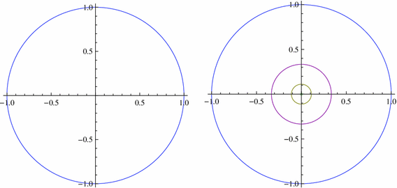
Note that \(A_0\) is an annulus and \(X_0\) is the union and \(X\) is a countable product of \(X_0\).
(a) The left circle is \(x^2+y^2=1\) and the right circle is \((x-1)^2+y^2=1/4\).
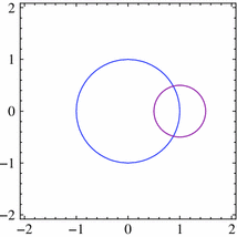
Let us observe that the length of the set \(\{x^2+y^2=1, \, (x-1)^2+y^2<r^2\}\) grows linearly when \(r\) is small enough. (b) The left circle is \(x^2+y^2=49\) and the right circle is \((x-1)^2+y^2=49\).
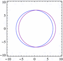
Since the left circle is large enough, the intersection of the large disk and the small one is sufficiently large.


References
Adams, D.R.: A note on Riesz potentials. Duke Math. J. 42, 765–778 (1975)
Adams, D.R., Hedberg, L.I.: Function Spaces and Potential Theory. Springer, Berlin (1996)
Almeida, A., Hasanov, J., Samko, S.: Maximal and potential operators in variable exponent Morrey spaces. Georgian Math. J. 15(2), 195–208 (2008)
Chiarenza, F., Frasca, M.: Morrey spaces and Hardy–Littlewood maximal function. Rend. Mat. Apple. 7(7), 273–279 (1987)
Duoandikoetxea, J.: Fourier analysis. In: Graduate Studies in Mathematics, vol. 29. American Mathematical Society, Providence (2001)
Edmunds, D.E., Krbec, M.: Two limiting cases of Sobolev imbeddings. Houst. J. Math. 21, 119–128 (1995)
Futamura, T., Mizuta, Y.: Continuity properties of Riesz potentials for functions in $L^{p(\cdot )}$ of variable exponent. Math. Inequal. Appl. 8(4), 619–631 (2005)
Futamura, T., Mizuta, Y., Shimomura, T.: Sobolev embedding for variable exponent Riesz potentials on metric spaces. Ann. Acad. Sci. Fenn. Math. 31, 495–522 (2006)
Futamura, T., Mizuta, Y., Shimomura, T.: Integrability of maximal functions and Riesz potentials in Orlicz spaces of variable exponent. J. Math. Anal. Appl. 366, 391–417 (2010)
Guliyev, V., Sawano, Y.: Linear operators on generalized Morrey spaces with non-doubling measures Publicationes Mathematicae Debrecen (2013, in press).
Gunawan, H., Sawano, Y., Sihwaningrum, I.: Fractional integral operators in nonhomogeneous spaces. Bull. Aust. Math. Soc. 80(2), 324–334 (2009)
Harjulehto, P., Hästö, P.: A capacity approach to the Poincaré inequality and Sobolev imbeddings in variable exponent Sobolev spaces. Rev. Mat. Complut. 17, 129–146 (2004)
Harjulehto, P., Hasto, P., Pere, M.: Variable exponent Lebesgue spaces on metric spaces: the Hardy–Littlewood maximal operator. Real Anal. Exch. 30(1), 87–103 (2004/2005).
Hedberg, L.I.: On certain convolution inequalities. Proc. Am. Math. Soc. 36, 505–510 (1972)
Kokilashvili, V., Meskhi, A.: Maximal functions and potentials in variable exponent Morrey spaces with non-doubling measure. Complex Var. Elliptic Equ. 55(8–10), 923–936 (2010)
Liu, L., Sawano, Y., Yang, D.: Morrey-type Spaces on Gauss Measure Spaces and Boundedness of Singular Integrals. J. Geom. Anal. (2013). doi: 10.1007/s12220-012-9362-9
Maeda, F-.Y., Mizuta, Y., Ohno, T.: Approximate identities and Young type inequalities in variable Lebesgue-Orlicz spaces $L^{p(\cdot )}(\log L)^{q(\cdot )}$. Ann. Acad. Sci. Fenn. Math. 35, 405–420 (2010)
Mizuta, Y.: Potential Theory in Euclidean Spaces. Gakkōtosho, Tokyo (1996)
Mizuta, Y., Nakai, E., Ohno, T., Shimomura, T.: An elementary proof of Sobolev embeddings for Riesz potentials of functions in Morrey spaces $L^{1,\nu,\beta }(G)$. Hiroshima Math. J. 38, 425–436 (2008)
Mizuta, Y., Nakai, E., Ohno, T., Shimomura, T.: Boundedness of fractional integral operators on Morrey spaces and Sobolev embeddings for generalized Riesz potentials. J. Math. Soc. Jpn. 62, 707–744 (2010)
Mizuta, Y., Nakai, E., Ohno, T., Shimomura, T.: Riesz potentials and Sobolev embeddings on Morrey spaces of variable exponent. Complex Var. Elliptic Equ. 56(7–9), 671–695 (2011)
Mizuta, Y., Shimomura, T.: Sobolev embeddings for Riesz potentials of functions in Morrey spaces of variable exponent. J. Math. Soc. Jpn. 60, 583–602 (2008)
Mizuta, Y., Shimomura, T.: Continuity properties for Riesz potentials of functions in Morrey spaces of variable exponent. Math. Inequal. Appl. 13, 99–122 (2010)
Mizuta, Y., Shimomura, T., Sobukawa, T.: Sobolev’s inequality for Riesz potentials of functions in non-doubling Morrey spaces. Osaka J. Math. 46, 255–271 (2009)
Morrey, C.B.: On the solutions of quasi-linear elliptic partial differential equations. Trans. Am. Math. Soc. 43, 126–166 (1938)
Nakai, E., Sawano, Y.: Hardy spaces with variable exponents and generalized Campanato spaces. J. Funct. Anal. 262(9), 3665–3748 (2012)
Nekvinda, A.: Hardy–Littlewood maximal operator on $L^{p(x)}$ (R). Math. Inequal. Appl. 7(2), 255–265 (2004)
Nakai, E.: Generalized fractional integrals on Orlicz–Morrey spaces. In: Banach and Function Spaces, pp 323–333. Yokohama Publications, Yokohama (2004)
Nazarov, F., Treil, S., Volberg, A.: Cauchy integral and Calderón–Zygmund operators on nonhomogeneous spaces. Internat. Math. Res. Not. 15, 703–726 (1997)
Nazarov, F., Treil, S., Volberg, A.: Weak type estimates and Cotlar inequalities for Calderön–Zygmund operators on nonhomogeneous spaces. Internat. Math. Res. Not. 9, 463–487 (1998)
Peetre, J.: On the theory of $L_{p,\lambda }$ spaces. J. Funct. Anal. 4, 71–87 (1969)
Sawano, Y.: Sharp estimates of the modified Hardy Littlewood maximal operator on the nonhomogeneous space via covering lemmas. Hokkaido Math. J. 34, 435–458 (2005)
Sawano, Y.: Generalized Morrey spaces for non-doubling measures. NoDEA Nonlinear Differ. Equ. Appl. 15(4–5), 413–425 (2008)
Sawano, Y., Sobukawa, T., Tanaka, H.: Limiting case of the boundedness of fractional integral operators on non-homogeneous space. J. Inequal, Appl (2006). (Art. ID 92470)
Sawano, Y., Tanaka, H.: Morrey spaces for non-doubling measures. Acta Math. Sin. (Engl. Ser.) 21, 1535–1544 (2005)
Sawano, Y., Wadade, H.: On the Gagliardo–Nirenberg type inequality in the critical Sobolev–Morrey space. J. Fourier Anal. Appl. 19(1), 20–47
Stein, E.M.: Singular Integrals and Differentiability Properties of Functions. Princeton University Press, Princeton (1970)
Terasawa, Y.: Outer measures and weak type (1,1) estimates of Hardy–Littlewood maximal operators. J. Inequal. Appl. (2006) (Art. ID 15063)
Trudinger, N.: On imbeddings into Orlicz spaces and some applications. J. Math. Mech. 17, 473–483 (1967)
Ziemer, W.P.: Weakly Differentiable Functions. Springer, New York (1989)
Acknowledgments
We are grateful to Professor F-.Y. Maeda for his fruitful discussion about the proof of Theorem 1.1.
Author information
Authors and Affiliations
Corresponding author
Rights and permissions
Open Access This article is distributed under the terms of the Creative Commons Attribution License which permits any use, distribution, and reproduction in any medium, provided the original author(s) and the source are credited.
About this article
Cite this article
Sawano, Y., Shimomura, T. Sobolev embeddings for Riesz potentials of functions in non-doubling Morrey spaces of variable exponents. Collect. Math. 64, 313–350 (2013). https://doi.org/10.1007/s13348-013-0082-7
Received:
Accepted:
Published:
Issue Date:
DOI: https://doi.org/10.1007/s13348-013-0082-7
Keywords
- Riesz potentials
- Maximal functions
- Sobolev’s inequality
- Trudinger’s inequality
- Continuity
- Morrey spaces of variable exponents
- Non-doubling measure
- Generalized smoothness