Structural optimization of unsymmetrical eccentric load steel box girder based on new swarm intelligence optimization algorithm

Abstract

The steel box girder structure is widely used in many engineering practices and it is therefore necessary to study the optimization and improvement of its structure. Firstly, a small-tonnage double-girder bridge crane was used as an example, with the box section parameters for one of the main girders as the design variables and weight reduction as the objective. The mathematical model for the optimization of this validation case was developed with the strength, stiffness and stability of the girder as the efficiency constraints. The next step was to go through two new swarm intelligence algorithms based on animal hunting behavior, Grey Wolf Optimizer (GWO) and Whale Optimization Algorithm (WOA), as well as two classical swarm algorithms, Particle Swarm Optimization (PSO) and Genetic Algorithm (GA). The optimization models of these four algorithms were simulated and analyzed by the finite element method, and the simulation results were compared. The feasibility and performance of these two new swarm intelligence algorithms in the structural optimization of asymmetric eccentrically loaded box girders were verified. Finally, these two new swarm intelligence algorithms were applied to the structural optimization of the main girder of a large-tonnage bridge crane.

1 Introduction

With the rapid development of modern industry, box girder structures are widely adopted in various engineering practices, such as bearing beam for working platforms, main beams for bridge crane and traffic trestle bridge. As a load-bearing structure, its design must first meet the requirements of stability and safety. On this premise, subsequent optimization of the design can be carried out. In previous box girder designs, designers have mostly relied on historical work experience to design the current box girder structure. This method often takes simple models such as rods as the basis for safe design, although the reliability of the designed structure can be guaranteed. However, it resulted in wastage of materials and failure to reduce energy consumption, which ultimately led to a decline of the performance of the whole machine.

Based on the above-mentioned problems, a large number of papers domestically and globally to study the optimization of box girders. Many scholars have attempted to optimize the parameters of stiffeners (as the size, position and number of stiffeners) in the box girder of the bridge crane to achieve lightweighting (Abid et al., 2008; Fu et al., 2013; Qin and Zhang et al., 2021a) Topology enhancement has also been used by a number of scholars to optimise the light-weighting of box girder of bridge crane with excellent outcomes (Jiao et al., 2014; Qin and Zhang et al., 2021b). In addition, a very efficient method of improving the dimensions of box girder cross-section can also be used to significantly reduce the weight of the complete machine. Savković et al. (2013) performed an optimization for the box section of main girder of an bridge crane using the Lagrange multiplier method and compared the results with the initial solution to verify the effectiveness of the method. Tian et al. (2013) firstly analyzed the stress in the main girder of the bridge crane and exploited the basis to optimize the box section size of the main girder. Finally, the weight of the whole machine was reduced. He et al. (2017) mixed the Particle Swarm Optimization into the composite method for complementary advantages and applied it to the improvement of the box section of the bridge crane main girder, which finally achieved the goal of lightening of the main girder. Savković et al. (2017) applied the biological heuristic algorithm to optimize the box section of the main girder of a single-beam bridge crane. The Cuckoo Search (CS), Bat Algorithm (BA) and Firefly Algorithm (FA) were applied and the optimization results were compared with several initial schemes for the single-beam bridge cranes to confirm the feasibility of the optimization method. Qi et al. (2021) implemented Specular Reflection Algorithm to optimize the main beam of the bridge crane using the cross-sectional area of the box girder as the objective function. As a result, the cross-sectional area of the box girder was reduced to 72.97% of its original size.

Meanwhile, the finite element method, as a mature modern computational method, has also been used by many scholars for the simulation analysis and optimization of bridge crane girders. He et al. (2013) carried out a finite element analysis of the bridge crane main girder under static and dynamic conditions, which provided a reference for the subsequent optimization of the main girder design. Liu et al. (2014) conducted a finite element analysis of the existing main girder of bridge crane and found that there was still a large safety margin in the existing structure. It was also that the follow-up optimization work must be based on the results of the previous numerical simulations, which in turn provided theoretical support for the light-weighting of the main girder of bridge crane. Li et al. (2011) used HyperWorks to dramatically reduce the weight of the main girder. Ning (2012) employed ANSYS to build a finite element model of a 200 T bridge crane main girder and optimized it by the first-order method to reduce the total volume of the main girder. Tong et al. (2013) utilized multidisciplinary techniques and finite element technology to optimize the bridge crane at the three levels, metal structure, transmission and electrical system design, ultimately achieving a reduction in overall weight. Qin and Gu et al. (2021) carried out a modal analysis of the crane using the finite element method, thus providing a reference for subsequent failure prevention.

In recent years, new swarm intelligence optimization algorithms have been proposed based on the hunting behavior of animals. The Grey Wolf Optimizer (GWO) (Mirjalili et al., 2014) and the Whale Optimization Algorithm (WOA) (Mirjalili et al., 2016), both new algorithms, have been widely used in diverse engineering practice due to their advantages of less parameters control, simplicity of operation and ability to jump out of local optimums with good results (Ling et al., 2019; Abderazek et al., 2019; Gharehchopogh & Gholizadeh, 2019; Ghalambaz et al., 2021). WOA and GWO, two new bioheuristics, are extensively used in engineering practice for their excellent optimization capabilities. However, few existing studies domestically and internationally have applied these two new algorithms to the optimization of box girder structures. Moreover, most of the box beams involved in the previous research are symmetrical structures, while the box beams with asymmetrical structures have a widespread application in practical engineering. Therefore, in this paper, these two new optimisation algorithms are applied to the lightweight optimization of asymmetric box girder structures, while two classical swarm algorithms, Particle Swarm Optimization (PSO) and Genetic Algorithm (GA), are used to optimize the same box girder, and the optimization results of these four algorithms are compared to discover the performance of the two new algorithms for the optimization of this structure. Finally, the optimized model is simulated and validated by finite element method.

2 Optimization mathematical model of asymmetric box beam

The overall box girder structure is shown in Fig. 1, and its cross section and force are shown in Fig. 2.

Fig. 1

Main girder of double-beam bridge crane

Fig. 2

Cross section of off-track box beam

2.1 Optimization design variables of asymmetric box beam

Because of the location of the equipment in which the box girder is located and associated working conditions, some box beams are asymmetric structures. In this paper, therefore, one main beams of the bridge crane are used as the object of research, keeping the same material and span as the original main beam in the successive optimization. Since the area of the main girder cross-section is proportional to the overall mass, the optimization of the quality of the main girder is translated into the optimization of the area of the main girder cross-section.According to Fig. 2, the design variables are:

$$ {\varvec{x}} = \left( {x_{1} ,x_{2} , \ldots ,x_{10} } \right)^{{\text{T}}} $$

(1)

where $x_{1}$-width of upper flange plate, $x_{2}$-width of lower flange plate, $x_{3}$-the distance between the main and auxiliary webs, $x_{4}$-thickness of upper flange plate, $x_{5}$-thickness of lower flange plate, $x_{6}$-the distance between the upper and lower flange plates, $x_{7}$-thickness of main web, $x_{8}$-thickness of auxiliary web, $x_{9}$-the distance between main web and left side of upper flange plate, $x_{10}$-the distance between main web and left side of lower flange plate.

Based on these ten variables, this paper designs an objective function and 36 constraint functions for subsequent optimization. The welding between various plates shall comply with the requirements of national standards, so it is not verified in this paper. The shape, position and quantity of the inner diaphragm and stiffener of the optimized box girder refer to the original box girder.

2.2 Objective function

The cross-sectional area of main girder is the objective function of optimization, and its expression is:

$$ f(x) = x_{1} x_{4} + x_{2} x_{5} + x_{6} (x_{7} + x_{8} ) $$

(2)

2.3 Constraint function

According to the relevant standards, the constraint functions are determined by the most unfavorable working condition of load, strength, stiffness, stability and other technical requirements in combination with the check of dangerous points in cross section.

2.3.1 Strength constraint

For such box girders, the main girder is subjected to both vertical and horizontal loads. However, the fatigue failure of the main girder often occurs near the positions which have the maximum normal stress and maximum shear stress or positions where both normal stress and shear stress are larger, and mainly occurs in the tension zone. The main beam of bridge crane has the maximum normal stress in the mid-span section, There is the maximum shear stress at the span end. Therefore, it is necessary to restrain the middle part of the span with normal stress and the end part with shear stress.

• 1. The internal force corresponding to the vertical load is calculated as follows. The uniformly distributed load of the main girder composed of the self-weight of the main girder and the rail weight of the crane trolley is shown in Fig. 3.

  Fig. 3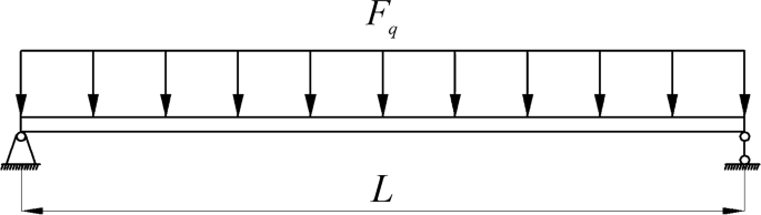

  

  Uniformly distributed load of main girder

On the mid-span of the main beam, the bending moment which is caused by the fixed loads is:

$$ M_{q} = \frac{{\phi_{4} F_{q} L^{2} }}{8} $$

(3)

where $\phi_{4}$-dynamic effect coefficient ($\phi_{4} = 1.19$), $F_{q}$-uniform load of main girder, $L$-span of main girder.

There are two fulcrums of the lifting trolley on the track of a main beam, and there are two balanced wheel pressures under each fulcrums. Here, the wheel pressure of four wheels are treated equally, and the position of wheel pressure action is determined according to the actual situation of the lifting trolley.

As shown in Fig. 4, when the wheel compression force is in the mid-span, Under this wheel, the maximum bending moment and corresponding shear force produced by the beam section are:

$$ M_{p} = \frac{{\sum {P(L - b_{1} )^{2} } }}{4L} - P_{1} a $$

(4)

$$ F_{p} \approx P_{1} $$

(5)

where $P_{1}$-single wheel pressure, $\sum P$-wheel pressing force ($\sum P$ = 4 $P_{1}$), $a$-the distance between two balanced wheel pressures at the same fulcrum, $b_{1}$-The distance between wheel pressing force and adjacent single wheel pressure.

Fig. 4

Wheel pressing force is in the mid-span

When the lifting trolley is located at the limit position ($c_{1}$) (as shown in Fig. 5), the sum of the maximum shear force and bending moment at the beam end are:

$$ F_{pc} = \frac{\sum P }{L}(L - b_{1} - a - c_{1} ) $$

(6)

$$ M_{pc} = F_{pc} c_{1} $$

(7)

Fig. 5

The lifting trolley is at the limit position ($c_{1}$)

When the lifting trolley is located in mid-span, the bending moment in mid-span of main girder caused by external load in vertical direction is:

$$ M_{x} = M_{q} + M_{pc} $$

(8)

When the lifting trolley is located at the span end, the shear force at the span end which is caused by the external load in the vertical direction is:

$$ F_{c} = F_{qc} + F_{pc} $$

(9)

• 2. The internal force corresponding to horizontal load is calculated as follows:

The calculation model of horizontal frame is shown in Fig. 6.

Fig. 6

Calculation model of horizontal rigid frame

The starting and braking inertia force of the lifting trolley (on a main beam) are:

$$ P_{H} = \frac{\sum P }{7}\frac{{n_{0} }}{{n_{{}} }} $$

(10)

$$ F_{H} = \frac{{F_{q} }}{7}\frac{{n_{0} }}{{n_{{}} }} $$

(11)

where $n$-total number of wheels of lifting trolley, $n_{0}$-number of driving wheels of lifting trolley.

When the lifting trolley is in mid-span, the horizontal bending moment in mid-span is:

$$ M_{H} = \frac{{P_{H} L}}{4}\left( {1 - \frac{1}{{2r_{1} }}} \right) + \frac{{F_{H} L^{2} }}{8}\left( {1 - \frac{2}{{3r_{1} }}} \right) $$

(12)

where $r_{1}$-calculation coefficient of rigid frame when the lifting trolley is in the mid-span.

Horizontal shear force in the mid-span is:

$$ F_{{_{PH} }} = \frac{1}{2}P_{H} $$

(13)

When the lifting trolley is located at the span end, the horizontal shear force at the span end is:

$$ F_{cH}^{\prime } = \frac{{F_{H} L}}{2} + P_{H} \left( {1 - \frac{{e_{1} }}{L}} \right) $$

(14)

where $e_{1}$-the fully loaded trolley is at the extreme position of the span end.

• 3. Strength conditions.

As shown in Fig. 7, establishing stress constraint functions at dangerous points 1, 2 and 3 in the middle span section of main beam.

$$ g_{1} (x) = \sigma_{1} - \left[ \sigma \right] \le 0 $$

(15)

$$ g_{2} (x) = \sigma_{2} - \left[ \sigma \right] \le 0 $$

(16)

$$ g_{3} (x) = \sigma_{3} - \left[ \sigma \right] \le 0 $$

(17)

Fig. 7

Location of dangerous points in main beam section

The constraint function of midpoint shear stress in main web and the constraint function of flange plate should also be considered.

$$ g_{4} (x) = \tau_{1} - \left[ \tau \right] \le 0 $$

(18)

$$ g_{5} (x) = \tau_{2} - \left[ \tau \right] \le 0 $$

(19)

In the above formulas (15) to (19),

$$ \sigma_{1} = \sqrt {\sigma_{0}^{2} + \sigma_{m}^{2} - \sigma_{0} \sigma_{m} + 3\tau^{2} } $$

(20)

$$ \sigma_{0} = \sigma_{01} + \sigma_{02} $$

(21)

where $\sigma_{01}$, $\sigma_{02}$-the stresses caused by vertical and horizontal bending moment respectively, $\sigma_{m}$-Local compressive stress at the edge of the main web, $\tau$-shear stress on the upper side of the main web.

$$ \sigma_{2} = \frac{{M_{x} Y_{2} }}{{I_{x} }} + \frac{{M_{H} X_{2} }}{{I_{y} }} $$

(22)

where $Y_{2}$-the distance from the centroid of the main beam section to the lower top surface of lower flange plate, $X_{2}$-the distance from the centroid of the main beam section to the right top surface of the lower flange plate.

$$ \sigma_{3} = 1.15\left[ {\frac{{M_{x} Y_{2} }}{{I_{x} }} + \frac{{M_{H} (X_{2} - \delta_{1} )}}{{I_{y} }}} \right] $$

(23)

where $\delta_{1}$-the distance from the right top surface of the lower flange plate to the outer side surface of the auxiliary web plate.

$$ \tau_{1} = \frac{{1.5F_{pc} }}{{h_{d} \sum \delta }} + \frac{{T_{n1} }}{{2A_{0} \delta }} $$

(24)

where $h_{d}$-end beam web height, $T_{n1}$-torque in the span end.

$$ \tau_{2} = \frac{{1.5F^{\prime}_{CH} }}{{x_{4} (x_{1} + x_{2} )}} + \frac{{T_{n1} }}{{2A_{0} x_{1} }} $$

(25)

2.3.2 Stiffness constraint

• 1. Static stiffness.

When four static wheel pressures act symmetrically on the center of the beam span, the mid span static deflection of beam is:

$$ Y = \frac{{2P_{`1} }}{{12EI_{x} }}\left[ {c\left( {\frac{3}{4}L^{2} - c^{2} } \right) + d\left( {\frac{3}{4}L^{2} - d^{2} } \right)} \right] $$

(26)

where $E$-the elastic modulus of steel, $c,d$-the distance from wheel to fulcrum.

• 2. Dynamic stiffness.

The vertical dynamic stiffness is represented by the vertical self-vibration frequency of the fully loaded trolley located in the span.

$$ f = \frac{1}{2\pi }\sqrt {\frac{{K_{e} }}{{m_{e} }}} $$

(27)

where $K_{e}$-equivalent stiffness of crane vibration system, $m_{e}$-equivalent mass at the maximum vibration point of the crane.

• 3. Establish stiffness constraint.

$$ g_{6} (x) = Y{ - }[Y_{s} ] \le 0 $$

(28)

$$ g_{7} (x) = [f] - f \le 0 $$

(29)

where $[Y_{S} ]$-allowable static deflection of main girder, $[f]$-the full-load natural vibration frequency control value of the crane(This paper takes 2 Hz).

Furthermore, the dynamic stiffness of the crane is not only related to the stiffness and quality of the main girder, but also to the lifting quality and the elastic elongation of the lifting wire rope. Therefore, considering the conditions of strength, stiffness, stability and lightest mass, the following constraints should be established and the ratio of the height to span of the main girder should be between 1/18 and 1/14:

$$ g_{8} \left( x \right) = \frac{{x_{4} + x_{5} + x_{6} }}{L} - \frac{1}{14} \le 0 $$

(30)

$$ g_{9} \left( x \right) = \frac{1}{18} - \frac{{x_{4} + x_{5} + x_{6} }}{L} \le 0 $$

(31)

2.3.3 Stability constraints

• 1. global stability constraint

The rigidity of the box beam is very large, If the aspect ratio of the beam $h/b \le 3$, the overall stability of the beam does not need to be checked:

$$ g_{10} (x) = \frac{{x_{4} + x_{5} + x_{6} }}{{x_{3} + x_{7} + x_{8} }} - 3 \le 0 $$

(32)

• 2. Local stability constraint of web.

If the plate thickness is determined by the local stability condition of the web, The thickness of the web shall not be less than $\left( {\frac{1}{200}\sim \frac{1}{160}} \right)x_{6}$, this article takes $x_{7,8} \ge \frac{{x_{6} }}{200}$:

$$ g_{11} \left( x \right) = \frac{{x_{6} }}{200} - x_{7} \le 0 $$

(33)

$$ g_{12} \left( x \right) = \frac{{x_{6}^{{}} }}{200} - x_{8} \le 0 $$

(34)

For the main web, it is subject to compressive stress, shear stress and local compressive stress respectively, and the stability constraints of the main web in the middle of the span are as follows:

$$ g_{13} \left( x \right) = \sqrt {\sigma_{0}^{2} + \sigma_{m}^{2} - \sigma_{0} \sigma_{m} + 3\tau_{m}^{2} } - \left[ {\sigma_{cr} } \right] \le 0 $$

(35)

For the auxiliary web, it is only subject to compressive stress and shear stress, and the stability constraints of the auxiliary web in the middle of the span are as follows:

$$ {\text{g}}_{14} \left( x \right) = \sqrt {\sigma_{n}^{2} + 3\tau_{{\text{n}}}^{2} } - \left[ {\sigma^{\prime}_{cr} } \right] \le 0 $$

(36)

In the above formula (35) ~ (36),

$$ \left[ {\sigma_{cr} } \right] = \frac{{\sigma_{cr} }}{n},\,\left[ {\sigma_{cr}^{\prime } } \right] = \frac{{\sigma_{cr}^{\prime } }}{n} $$

(37)

$$ \sigma_{cr} = \frac{{\sqrt {\sigma_{0}^{2} + \sigma_{m}^{2} - \sigma_{0} \sigma_{m} + 3\tau_{m}^{2} } }}{{\frac{1 + \psi }{4}\left( {\frac{{\sigma_{0} }}{{\sigma_{0cr} }}} \right) + \sqrt {\left[ {\frac{3 - \psi }{4}\left( {\frac{{\sigma_{0} }}{{\sigma_{0cr} }}} \right) + \frac{{\sigma_{m} }}{{\sigma_{mcr} }}} \right]^{2} + \left( {\frac{{\tau_{m} }}{{\tau_{mcr} }}} \right)^{2} } }} $$

(38)

$$ \sigma_{cr}^{\prime } = \frac{{\sqrt {\sigma_{{\text{n}}}^{2} + 3\tau_{n}^{2} } }}{{\frac{1 + \psi }{4}\left( {\frac{{\sigma_{{\text{n}}} }}{{\sigma_{ncr} }}} \right) + \sqrt {\left[ {\frac{3 - \psi }{4}\left( {\frac{{\sigma_{n} }}{{\sigma_{ncr} }}} \right)} \right]^{2} + \left( {\frac{{\tau_{n} }}{{\tau_{ncr} }}} \right)^{2} } }} $$

(39)

where $n$-safety factor, $\tau_{{\text{m}}}$-Average shear stress of main web, $\psi$-Ratio of bending stress on two edges of central section of main web, $\sigma_{{{\text{ocr}}}}$-Critical compressive stress of main web, $\tau_{{{\text{mcr}}}}$-Critical shear stress of main web, $\sigma_{{{\text{mcr}}}}$-Critical local compressive stress of main web, $\tau_{{\text{n}}}$-Average shear stress of auxiliary web, $\sigma_{{\text{n}}}$-Normal stress on both sides of auxiliary web ($\sigma_{{\text{n}}} = \sigma_{01} + \sigma_{02} \frac{{X_{2} - \delta_{1} - \left( {x_{8} /2} \right)}}{{x_{2} - X_{2} - x_{10} - \left( {x_{7} /2} \right)}}$), $\sigma_{{{\text{ncr}}}}$-Critical compressive stress of auxiliary web, $\tau_{{{\text{ncr}}}}$-Critical shear stress of auxiliary web.

Where:

$$ \sigma_{{{\text{0cr}}}} = \mu K_{\sigma } \sigma_{E} ,\;\sigma_{{{\text{ncr}}}} = \mu K_{\sigma } \sigma_{E} $$

(40)

$$ \tau_{{{\text{mcr}}}} = \mu K_{\tau } \sigma_{E} ,\;\tau_{{{\text{ncr}}}} = \mu K_{\tau } \sigma_{E} $$

(41)

$$ \sigma_{{{\text{mcr}}}} = \mu K_{m} \sigma_{E} $$

(42)

where $\mu$-Elastic embedment coefficient of plate edge, $K_{\sigma }$, $K_{\tau }$, $K_{{\text{m}}}$-Buckling coefficient of simply supported plate with four sides, $\sigma_{{\text{E}}}$-Euler stress of simply supported plates with four sides ($\sigma_{{\text{E}}} = 18.62\left( {\frac{{100x_{7,8} }}{{b^{\prime } }}} \right)$, $b^{\prime }$-Distance between longitudinal stiffeners).

2.3.4 dimensional constraints

In order to meet the actual situation, it is necessary to restrict the size of the box beam.

$$ g_{15} \left( x \right) = x_{3} + x_{9} + x_{7} + x_{8} - x_{1} \le 0 $$

(43)

$$ g_{16} \left( x \right) = x_{3} + x_{10} + x_{7} + x_{8} - x_{2} \le 0 $$

(44)

$$ g_{16 + m} \left( x \right) = x_{m\min } - x_{m} \le 0,\;(m = 1,2, \ldots ,10) $$

(45)

$$ g_{26 + m} \left( x \right) = x_{m} - x_{m\max } \le 0,\;(m = 1,2, \ldots ,10) $$

(46)

The above constraint functions are established according to ISO 8686–1:2012 (Cranes—Design principles for loads and load combinations—Part 1: General) and ISO 20332:2013 (Cranes—Proof of competence of steel structures).

3 Intelligent swarm optimization algorithm

GWO and WOA are both new algorithms developed in recent years inspired by the predation behavior of animal groups. This paper will briefly introduce these two algorithms and apply them to the examples cited in this paper.

3.1 Grey Wolf Optimizer (GWO)

There are three wolves in the pack: α, β and δ. α is the king and is ranked first in the social hierarchy of the pack, while β and δ are ranked second and third respectively. Therefore, β needs to obey α, and δ needs to obey both α and β. The remaining individuals are labelled as ω at the bottom of the social hierarchy (these three wolves represent the three best solutions and ω the candidate solutions). These three wolves lead the other wolves to their prey, and the hunting process is the procedure of finding the optimal solution. The specific optimization procedure includes steps such as social stratification, tracking, encircling and attacking prey.

When encircling prey, wolves constantly update their position to get closer to the prey. This behavior can be represented by the following mathematical model:

$$ \vec{O} = \left| {\vec{E} \cdot \vec{X}_{{\text{q}}} (t) - \vec{X}_{{\text{g}}} (t)} \right| $$

(47)

$$ \vec{X}_{{\text{g}}} (t + 1) = \vec{X}_{{\text{q}}} (t) - \vec{G} \cdot \vec{O} $$

(48)

Equation (47) is the meaning of the distance between individual and prey, and Eq. (48) represents the update formula of grey wolf's position.

Where $t$-the current iterative algebra, $\vec{G}$ and $\vec{E}$-coefficient vectors, $\vec{X}_{{\text{g}}}$-the position vectors of grey Wolf, $\vec{X}_{{\text{q}}}$-the position vectors of prey. Calculation formulas of $\vec{G}$ and $\vec{E}$ are given as follows:

$$ \vec{G} = 2{\vec{\text{i}}} \cdot \vec{s}_{1} - \vec{i} $$

(49)

$$ \vec{E} = 2 \cdot {\vec{\text{s}}}_{2} $$

(50)

where ${\vec{\text{i}}}$-a convergence factor and during the iteration, its value linearly decreases from 2 to 0, ${\vec{\text{s}}}_{1} ,\vec{s}_{2} \in \left[ {0,1} \right]$.

As the position of prey is unknown (the best solution is unknown), in order to simulate the search behavior of wolves, the three best performing wolves (α, β and δ) need to be selected in each iteration and then the location of the prey is judged by α, β and δ. In turn, the other candidate wolves randomly update their positions in the vicinity of the prey under the guidance of these three wolves:

$$ \left\{ {\begin{array}{*{20}c} {\vec{O}_{\alpha } = \left| {\vec{E}_{1} \cdot \vec{X}_{\alpha } - \vec{X}_{{\text{g}}} } \right|} \\ {\vec{O}_{\beta } = \left| {\vec{E}_{2} \cdot \vec{X}_{\beta } - \vec{X}_{g} } \right|} \\ {\vec{O}_{\delta } = \left| {\vec{E}_{3} \cdot \vec{X}_{\delta } - \vec{X}_{g} } \right|} \\ \end{array} } \right. $$

(51)

where $\vec{O}_{\alpha }$, $\vec{O}_{\beta }$ and $\vec{O}_{\delta }$-the distances between other individuals and three leader wolves, $\vec{X}_{\alpha }$, $\vec{X}_{\beta }$ and $\vec{X}_{\delta }$-the current positions of three leader wolves respectively, $\vec{E}_{1}$, $\vec{E}_{2}$ and $\vec{E}_{3}$ is a random vector, $\vec{X}_{{\text{g}}}$ is the current position of the grey wolf.

$$ \left\{ {\begin{array}{*{20}c} {\vec{X}_{g1} = \vec{X}_{\alpha } - G_{1} \cdot (\vec{O}_{\alpha } )} \\ {\vec{X}_{g2} = \vec{X}_{\beta } - G_{2} \cdot (\vec{O}_{\beta } )} \\ {\vec{X}_{g3} = \vec{X}_{\delta } - G_{3} \cdot (\vec{O}_{\delta } )} \\ \end{array} } \right. $$

(52)

$$ \vec{X}_{g} (t + 1) = \frac{{\vec{X}_{g1} + \vec{X}_{g2} + \vec{X}{}_{g3}}}{3} $$

(53)

Equation (52) defines step size and direction of individual in the wolves to the three leader wolves respectively, Eq. (53) is the meaning of the final position of individual.

Grey wolves need to approach and attack prey to end hunting, and This behavior is simulated by reducing the value of ${\vec{\text{i}}}$, because from the formula (49), $\vec{G}$ is a random vector in the interval $\left[ { - i,i} \right]$, and ${\vec{\text{i}}}$ decreases linearly in the iteration. Therefore, the fluctuation range of $\vec{G}$ will also decrease with the decrease of ${\vec{\text{i}}}$. when $\left| {\mathop{G}\limits^{\rightharpoonup} } \right| < 1$, wolves attack prey collectively. When $\left| {\mathop{G}\limits^{\rightharpoonup} } \right| > 1$, the wolves will leave their prey and search and attack again.

3.2 Whale Optimization Algorithm (WOA)

3.2.1 Surround the prey

This mechanism is the same as GWO. In WOA, the mathematical expression of this behavior is:

$$ \vec{O} = \left| {\overline{E} \cdot \vec{X}^{ * } (t) - \vec{X}_{W} (t)} \right| $$

(54)

$$ \vec{X}_{W} (t + 1) = \vec{X}^{ * } (t) - \vec{G} \cdot \vec{O} $$

(55)

where $t$-iterative algebra at present, $\vec{G}$ and $\vec{E}$-a coefficient vector, $\vec{X}^{ * } (t)$-Optimal positions of individual in current whale population, $\vec{X}_{W} (t)$-the position of the individual whale group at present. The calculation formula of $\vec{G}$ and $\vec{E}$ are as follows:

$$ \vec{G} = 2\vec{i} \cdot \vec{s}_{1} - \vec{i} $$

(56)

$$ \vec{E} = 2 \cdot \vec{s}_{2} $$

(57)

where $\vec{i}$-a vector and during the iteration, Its value linearly decreases from 2 to 0, $\vec{s}_{1}$ and $\vec{s}_{2}$-a random vector between [0,1].

3.2.2 Bubble net attack mode

There are two ways to model the bubble net behavior of humpback whales:

• 1. Contraction surrounding mechanism.

The mechanism is achieved through reducing $\vec{i}$ in Eq. (56).And the decrease of $\vec{i}$ also drives the decrease of $\vec{G}$.

• 2. Spiral update position.

By creating a spiral equation to simulate this behavior. The equation is shown below:

$$ \vec{X}_{W} (t + 1) = \vec{O}^{\prime } \cdot e^{b\varsigma } \cdot \cos (2\pi \zeta ) + \vec{X}^{ * } (t) $$

(58)

where $\zeta$-a random value between-1 and 1, $\vec{O}^{\prime } = \left| {\vec{X}^{ * } (t) - \vec{X}_{W} (t)} \right|$ represents the distance between the $i$ th whale and prey, $b$-the constant defining the spiral shape.

Because two attack modes are carried out simultaneously, it can be assumed that the probability of occurrence of the two modes is the same, both of which are 50%. The mathematical model is shown below:

when $p < \frac{1}{2}$:

$$ \vec{X}_{W} (t + 1) = \vec{X}^{ * } (t) - \vec{G} \cdot \vec{O} $$

(59)

when $p \ge \frac{1}{2}$:

$$ \vec{X}_{W} (t + 1) = \vec{O}^{\prime } \cdot e^{b\zeta } \cdot \cos (2\pi \zeta ) + \vec{X}^{ * } (t) $$

(60)

where $p$ is a random value between 0 and 1.

3.2.3 Searching for prey

The global search ability of WOA is realized by searching prey mechanism. The mathematical model is as follows:

$$ \vec{O} = \left| {\vec{E} \cdot \vec{X}_{rand} - \vec{X}_{W} } \right| $$

(61)

$$ \vec{X}_{W} (t + 1) = \vec{X}_{rand} - \vec{G} \cdot \vec{O} $$

(62)

where $\vec{X}_{rand}$ is the random position vector.

4 Performance verification of new swarm intelligence algorithm for structural optimization of asymmetric box girders

Taking the 32t/8t small-tonnage asymmetric box girder as a verification case, and the optimization results of Particle Swarm Optimization (PSO) and Genetic Algorithm (GA) were compared to verify the performance of Grey Wolf Optimizer (GWO) and Whale Optimization Algorithm (WOA). For these four algorithms, the constraint conditions were introduced by adding penalty function.

For the four algorithms used to optimize the box beam in this paper, the control parameters are:

$$ \begin{array}{*{20}c} {{\text{SearchAgent}}\_{\text{no}}\, = \,{5}0\left( {{\text{Population}}\;{\text{size}}} \right);} \\ {{\text{Max}}\_{\text{iteration}}\, = \,{1}000\left( {{\text{Number}}\;{\text{of}}\;{\text{iterations}}} \right);} \\ {{\text{dim}}\, = \,{1}0\left( {\text{Number of variables}} \right).} \\ \end{array} $$

For Particle Swarm Optimization (PSO), some control parameters are:

$$ \begin{array}{*{20}c} {{\text{vlimit}}\_{\text{max}}\, = \,0.0{1}*{\text{ub}}\left( {{\text{Speed}}\;{\text{limit}}} \right);} \\ {{\text{vlimit}}\_{\text{min}}\, = \,\, - \,{\text{vlimit}}\_{\text{max}};} \\ {{\text{P}}\_{1}\, = \,0.{8}\left( {{\text{Inertia}}\;{\text{weight}}} \right);} \\ {{\text{P}}\_{2}\, = \,{1}.{4}\left( {{\text{Self}} - {\text{learning}}\;{\text{factor}}} \right);} \\ {{\text{P}}\_{3}\, = \,{1}.{4}\left( {{\text{Group}}\;{\text{learning}}\;{\text{factor}}} \right).} \\ \end{array} $$

For Genetic Algorithm (GA), some control parameters are:

$$ \begin{array}{*{20}l} {{\text{gaDat}}.{\text{Pc}}\, = \,0.{8}\left( {\text{Crossover probability}} \right);} \hfill \\ {{\text{gaDat}}.{\text{Pm}}\, = \,0.{1}\left( {\text{Mutation probability}} \right).} \hfill \\ \end{array} $$

The upper and lower limits of variables in the box girder structure of this case are as follows ($x_{1} \sim x_{10}$):

$$ \begin{aligned} & {\text{lb}} = \left[ {\begin{array}{*{20}l} {0.65} \hfill & {0.56} \hfill & {0.5222} \hfill & {0.007} \hfill & {0.007} \hfill & {1.12} \hfill & {0.0056} \hfill & {0.0042} \hfill & {0.105} \hfill & {0.014} \hfill \\ \end{array} } \right]\left( {{\text{lower}}\;{\text{limit}}\;{\text{of}}\;{\text{variable}}} \right); \\ & {\text{ub}} = \left[ {\begin{array}{*{20}l} {1.2} \hfill & {1.04} \hfill & {0.97} \hfill & {0.013} \hfill & {0.013} \hfill & {2.08} \hfill & {0.01} \hfill & {0.0078} \hfill & {0.195} \hfill & {0.026} \hfill \\ \end{array} } \right]\left( {{\text{upper}}\;{\text{limit}}\;{\text{of}}\;{\text{variable}}} \right). \\ \end{aligned} $$

4.1 Design variables required for optimization

The crane design parameters are shown in Table 1.

Table 1 32 T Crane design parameters

Under the premise of satisfying the constraints, the optimization results are compromised according to the relevant standards and regulations. The thickness of the web and flange plate is taken as an integer depending on the plate specification, and the height of the web and the width of the flange plate are taken as an integer multiple of 5.

4.2 Optimization results and verification

4.2.1 Optimization results

The optimization results of the four algorithms are shown in Table 2 below, and the iterative curve diagram is shown in Fig. 8.

Table 2 Optimization results of main beam of 32 T bridge crane

Fig. 8

Iterative curve diagram a GWO; b WOA; c PSO; d GA

4.2.2 Finite element verification and comparison of optimization results

The finite element method, as a modern computational method, is widely used in engineering practice because of its high accuracy and applicability for various complex shapes. Therefore, this paper extends the finite element method to complex box girder structures, not only to verify the reliability of the algorithm’s optimization results, but also to visualize the performance of the new swarm intelligence algorithm in optimizing such structures.

• 1. Stress verification of box beam optimized by GWO and WOA in mid-span and end-span working conditions.

When the fully loaded trolley is located in the middle of the span, the stress nephogram for the original box girder and the box girder optimized by GWO and WOA are shown in Fig. 9a–c respectively. The deformation nephograms for the original box beam and that optimized by GWO and WOA are shown in Fig. 9d–f respectively. When the fully loaded trolley is at the span end, the stress nephogram for the original box girder and that optimized by GWO and WOA are shown in Fig. 10a–c respectively.The deformation nephograms for the original, optimized by GWO and WOA box beam are shown in Fig. 10d–f respectively.

Fig. 9

Stress nephogram of mid-span working condition a original box girder; b box beam optimized by GWO; c box beam optimized by WOA; total deformation nephogram of mid-span working condition d original box girder; e box beam optimized by GWO; f box beam optimized by WOA

Fig. 10

Stress nephogram of span-end working condition a original box beam; b box beam optimized by GWO; c box beam optimized by WOA; total deformation nephogram of span-end working condition d original box girder; e box beam optimized by GWO; f box beam optimized by WOA

The factor of safety is 1.48 and the allowable stress is 157 MPa ($233/1.48 \approx 157.4$), According to Figs. 9b, c and 10b, c, the maximum stress and static strength of the beam optimized by GWO and WOA under the two extreme operating conditions meet the design requirements. The box girder has a working class of A6 and a span of 25.5 m. Its permissible static deflection is 31 mm ($25500/800 \approx 31.8$), Following Figs. 9e–f and 10e, f, the maximum deflection of the beam optimized by GWO and WOA under the two extreme working conditions are less than the permissible static deflection, indicating that it meets the design requirements for static stiffness.

• 2. Stress verification of box beam optimized by PSO and GA in mid-span and end-span working conditions.

When the fully loaded trolley is located in the middle of the span, the stress nephogram for the box girder optimized by PSO and GA are shown in Fig. 11a, b respectively. The deformation nephogram for box girder optimized by PSO and GA are shown in Fig. 11e, f respectively. When the fully loaded trolley is located at the end of the span, the stress nephogram for the box girder optimized by PSO and GA are shown in Fig. 11c, d respectively. The deformation nephogram for the box beam optimized by PSO and GA are shown in Fig. 11g, h respectively.

Fig. 11

Stress nephogram of mid-span working condition a box beam optimized by PSO; b box beam optimized by GA; stress nephogram of span-end working condition c box beam optimized by PSO; d box beam optimized by GA; total deformation nephogram of mid-span working condition e box beam optimized by PSO; f box beam optimized by GA; total deformation nephogram of span-end working condition g box beam optimized by PSO; h box beam optimized by GA

The maximum stress of the optimized beam of PSO and GA under two extreme working conditions shown in Fig. 11a–d are less than the allowable stress, which meets the requirements of static strength design. Figure 11e–h show that the maximum deformation of the optimized beam of PSO and GA under two extreme working conditions are less than its allowable static deflection,which meets the requirements of static stiffness design.

• 3. Modal verification of four optimization algorithms.

Modal analysis is an engineering method for studying the inherent properties of a structure. Modal analysis of optimized box girder can effectively avoid the resonance phenomenon under external excitation. As bridge crane is a large lifting equipment, the vibration frequency is low and the low-order mode occupies the main position in the dynamic response of the structure. Therefore, this paper used the first six-order frequency of the optimized box girder for calculation. The results of the first six-order modal analysis of the optimized main girder are shown in Table 3, and the modal vibration diagram only shows the first two orders, as shown in Fig. 12 below.

Table 3 The results of the first six-order modal analysis of the optimized main beam

Fig. 12

Modal analysis diagram a GWO first-order mode; b WOA first-order mode; PSO first-order mode; d GA first-order mode; e GWO second-order mode; f WOA second-order mode; g PSO second-order mode; h GA second-order mode

The dynamic stiffness of the bridge crane structure should not be less than the control value of the natural vibration frequency when the fully loaded trolley is in the mid-span working condition ($\left[ f \right] = 2\,{\text{Hz}}$). As shown in Table 3, the minimum natural frequencies of the first six modes of these four optimized beams are all greater than 2 Hz, so the box beams optimized by these four algorithms all meet requirements of the dynamic stiffness design.

The results of finite element analysis show that the box girder structures optimized by these four optimization algorithms all meet the design requirements. The actual optimization amount of WOA is close to that of GWO, but both of them are obviously superior to the other two classical algorithms. At the same time, the maximum stress of box beams optimized by GWO and WOA under extreme working conditions is close to its allowable stress, while box beams optimized by PSO and GA still have a lot of safety margin. This also indirectly verifies the performance of these two new swarm algorithms for this structure optimization.

5 Optimization of structural engineering problems of heavy-load asymmetric box girder

The 300t/140t heavy-load asymmetric box girder was optimized by four algorithms, and the optimized results of the four algorithms were compared. Finally, the optimization models of GWO and WOA were verified by finite element method.

5.1 Design variables required for optimization

The upper and lower limits of variables in the box girder structure of this case are as follows ($x_{1} \sim x_{10}$):

$$ \begin{aligned} & {\text{lb}} = \left[ {\begin{array}{*{20}l} {1.5} \hfill & {1.4} \hfill & {1.38} \hfill & {0.014} \hfill & {0.014} \hfill & 2 \hfill & {0.009} \hfill & {0.007} \hfill & {0.13} \hfill & {0.014} \hfill \\ \end{array} } \right]\left( {{\text{lower}}\;{\text{limit}}\;{\text{of}}\;{\text{variable}}} \right); \\ & {\text{ub}} = \left[ {\begin{array}{*{20}l} {2.8} \hfill & {2.6} \hfill & {2.5} \hfill & {0.026} \hfill & {0.026} \hfill & {3.8} \hfill & {0.019} \hfill & {0.013} \hfill & {0.25} \hfill & {0.026} \hfill \\ \end{array} } \right]\left( {{\text{upper}}\;{\text{limit}}\;{\text{of}}\;{\text{variable}}} \right). \\ \end{aligned} $$

The crane design parameters are shown in Table 4.

Table 4 300 T Crane design parameters

5.2 Optimization results and verification

5.2.1 Optimization results

The optimization results of the four algorithms are shown in Table 5 below, and the iterative diagram of the algorithms is shown in Fig. 13.

Table 5 Optimization results of main beam of 300 T bridge crane

Fig. 13

Iterative curve diagram a GWO; b WOA; c PSO; d GA

5.2.2 Finite element verification of optimization results

• 1. Stress verification in mid-span working condition

The stress nephogram for the original box girder and the box girder optimized by GWO and WOA are shown in Fig. 14a–c respectively. The deformation nephogram for the original box beam and the box beam optimized by GWO and WOA are shown in Fig. 14d–f respectively.

Fig. 14

Stress nephogram of mid-span working condition a original box girder; b box beam optimized by GWO; c box beam optimized by WOA; total deformation nephogram of mid-span working condition d original box girder; e box beam optimized by GWO; f box beam optimized by WOA

Figure 14a–c show that when the fully loaded trolley is in the mid-span working operation, the maximum stress in the original box beam is about 193 MPa, the value for that optimized by GWO and WOA is about 229 MPa and 222MP rspectively. the safety factor is 1.48 and the allowable stress is 233 MPa ($345/1.48 \approx 233.1$). The results optimized by both algorithms are less than the allowable stress and meet the requirements of static strength design. Figure 14d–f show that the maximum deformation of the original box beam is 11.18 mm under above condition, while the maximum deformation for that optimized by GWO and WOA is 19.76 mm and 20.04 mm rspectively. and the working class of the box beam is A6, its span is 28.9 m,The allowable static deflection is 36 mm ($28900/800 \approx 36.1$), the results optimized by both algorithms are lower than the permissible static deflection and fulfill the requirements for static stiffness design.

• 2. Stress verification in end-span working condition.

The stress nephogram for the original box girder and the box girder optimized by GWO and WOA are shown in Fig. 15a–c respectively. The deformation nephogram for the original box beam and the box beam optimized by GWO and WOA are shown in Fig. 15d–f respectively.

Fig. 15

Stress nephogram of span-end working condition a original box beam; b box beam optimized by GWO; c box beam optimized by WOA; total deformation nephogram of span-end working condition d original box girder; e box beam optimized by GWO; f box beam optimized by WOA

Figure 15a–c show that the maximum stress of the original box beam is about 163 MPa when the fully loaded trolley is in the span-end working condition, the value for that optimized by GWO and WOA is about 173 MPa and 170 MPa respectively. The results optimized by both algorithms are less than the allowable stress, which meets the requirements of static strength design. Figure 15d–f show that the maximum deformation of the original box girder is 5.07 mm,The maximum deformation of the box beam optimized by GWO and WOA is 8.65mmand 8.43 mm respectively. The results optimized by both algorithms are lower than the permissible static deflection, which meets the requirements of static stiffness design.

• 3. Modal analysis.

The results of the first six-order modal analysis of the optimized main girder are shown in Table 6, and the modal shape diagram only show the first two orders, and are shown in Fig. 16 below.

Table 6 The results of the first six-order modal analysis of the optimized main beam

Fig. 16

Modal analysis diagram a GWO first-order mode; b GWO second-order mode; c WOA first-order mode; d WOA second-order mode

It can be seen from Table 6, the minimum natural frequencies of the first six-order modes of both optimized beams are first-order modes. Figure 16a shows the frequency of the first-order mode of the box beam optimized by GWO is $f = 10.474\;{\text{Hz}}$. Figure 16c shows the frequency of the first-order mode of the box beam optimized by WOA is $f = 10.318\;{\text{Hz}}$. Both optimised beams have minimum natural frequencies greater than 2 Hz for the first six orders of modalities, so as a result each of the GWO and WOA optimized box beams meet the dynamic stiffness design requirements.

The above results show that the maximum stress, deformation and modal analysis results of the main girder optimized by GWO and WOA under two extreme working conditions all meet the requirements of the design, which shows that the optimized results are desirable. And comparing the optimization amount with PSO and GA, it shows that GWO and WOA have stronger optimization ability in this kind of box girder structure.

6 Conclusion

• 1. The results of the above analysis show that the optimization of asymmetrically eccentrically loaded box girders using GWO and WOA is desirable and the optimization amounts of the both algorithms are similar. Compared to the original box girder, the optimization amount of both two algorithms is about 12 ~ 17%;

• 2. As new swarm intelligence algorithms, GWO and WOA are not only operationally simpler than conventional PSO and GA, but also have fewer parameters to be controlled. Moreover, in the optimization of asymmetrically eccentrically loaded box girder structures, these two new algorithms outperform PSO and GA by approximately 2 ~ 4%.

• 3. Simulations of box beams analysed with these four algorithms using the finite element method not only verify the reliability of the optimization results, but also provide a more intuitive picture of the optimization performance of the two new algorithms for this type of structure.

This paper provides a new idea and method for lightweight design of this kind of box girder, which makes it possible to design the structure at lower cost in the design work of similar box girder in the future, which also reflects the practical engineering significance of this paper.

References

Abderazek, H., Yildiz, A. R., & Mirjalili, S. (2019). Comparison of recent optimization algorithms for design optimization of a cam-follower mechanism. Knowledge-Based Systems, 191, 105237.
Abid, M., Akmal, M. H., & Parvez, S. (2008). Design optimization of box type girder of an overhead crane. Iranian Journal of Science and Technology Transactions of Mechanical Engineering, 39(M1), 101–112.
Fu, W., Cheng, W., Yu, L., & Pu, D. (2013). Bionics design of transverse stiffener in the upright rail box girder based on bamboo strucure. Xinan Jiaotong Daxue Xuebao/journal of Southwest Jiaotong University, 48(2), 211–216.
Ghalambaz, M., Yengeje, H. R. J., & Davami, A. H. (2021). Building energy optimization using grey wolf optimizer (gwo). Case Studies in Thermal Engineering, 27(4), 101250.
Gharehchopogh, F. S., & Gholizadeh, H. (2019). A comprehensive survey: Whale optimization algorithm and its applications. Swarm and Evolutionary Computation, 48, 1–24.
Gu, J., Qin, Y., Xia, Y., Wang, J., Gao, H., & Jiao, Q. (2021). Failure analysis and prevention for tower crane as sudden unloading. Journal of Failure Analysis and Prevention., 21, 1590–1595.
He, Y., Wang, Z., Detand, J., Ruxu, D., Self, J. A., & Gunsing, J. (2017). Complex method mixed with pso applying to optimization design of bridge crane girder. Matec Web of Conferences, 104, 02010.
He, Y. B., Zhang, Y., Yang, B. K., Liu, S. W., & Chen, D. F. (2013). Finite element analysis in dynamic conditions of bridge crane beam. In Applied Mechanics and Materials (Vol. 331, pp. 70–73). Trans Tech Publications Ltd.
Jiao, H., Zhou, Q., Qinglong, W. U., Wenjun, L. I., & Ying, L. I. (2014). Periodic topology optimization of the box-type girder of bridge crane. Journal of Mechanical Engineering, 50(23), 134.
Li, X., Yuan, X., Zhen, Y., & Fei, S. (2011). Research on the structure optimization design of bridge crane. In International conference on remote sensing. IEEE.
Ling, A. W., Ramachandaramurthy, V. K., Walker, S. L., Taylor, P., & Sanjari, M. J. (2019). Optimal placement and sizing of battery energy storage system for losses reduction using whale optimization algorithm. The Journal of Energy Storage, 26, 100.
Liu, P., Xing, L., Liu, Y., & Zheng, J. (2014). Strength analysis and optimal design for main girder of double-trolley overhead traveling crane using finite element method. Journal of Failure Analysis & Prevention, 14(1), 76–86.
Mirjalili, S., & Lewis, A. (2016). The whale optimization algorithm. Advances in Engineering Software., 95, 51–67.
Mirjalili, S., Mirjalili, S. M., & Lewis, A. (2014). Grey wolf optimizer. Advances in Engineering Software., 69, 46–61.
Ning, Z. Y. (2012). Structural optimization research on girder of 200t bridge crane based on ansys. Advanced Materials Research, 430–432, 1708–1711.
Qi, Q., Xu, H., Xu, G., Dong, Q., & Xin, Y. (2021). Comprehensive research on energy-saving green design scheme of crane structure based on computational intelligence. AIP Advances, 11(7), 075314.
Savković, M. M., Bulatović, R. R., Gašić, M. M., Pavlović, G. V., & Stepanović, A. Z. (2017). Optimization of the box section of the main girder of the single-girder bridge crane by applying biologically inspired algorithms. Engineering structures, 148, 452–465.
Savković, M. M., Gašić, M. M., Ćatić, D. M., Nikolić, R. R., & Pavlović, G. V. (2013). Optimization of the box section of the main girder of the bridge crane with the rail placed above the web plate. Structural and Multidisciplinary Optimization, 47(2), 273–288.
Tian, G. F., Zhang, S. Z., & Sun, S. H. (2013). The optimization design of overhead traveling crane’s box girder. Advanced Materials Research, 605–607, 3–8.
Tong, Y., Wei, Y., Zhen, Y., Li, D., & Li, X. (2013). Research on multidisciplinary optimization design of bridge crane. Mathematical Problems in Engineering, 2013(pt.6), 211–244.
Zhang, H., Qin, Y., Gu, J., Gao, H., & Mi, C. (2021a). Layout optimization of stiffeners in heavy-duty thin-plate box grider. KSCE Journal of Civil Engineering, 25, 3078–3083.
Zhang, Y., Qin, Y., Gu, J., Jiao, Q., & Zheng, H. (2021b). Topology optimization of unsymmetrical complex plate and shell structures bearing multicondition overload. Journal of Mechanical Science and Technology, 35, 3497–3506.
Funding
The author(s) disclosed receipt of the following financial support for the research, authorship, and/or publication of this article: This work was supported by the Shanxi Provincial Key Research and Development Project (201903D121067), the National Natural Science Foundation of China (51275329) and the Fund for Shanxi ‘1331’ Project’ Key Subjects Construction (1331KSC).
Author information
Authors and Affiliations
Corresponding author
Additional information
Publisher's Note
Springer Nature remains neutral with regard to jurisdictional claims in published maps and institutional affiliations.
Rights and permissions
Springer Nature or its licensor holds exclusive rights to this article under a publishing agreement with the author(s) or other rightsholder(s); author self-archiving of the accepted manuscript version of this article is solely governed by the terms of such publishing agreement and applicable law.
About this article
Cite this article
Su, S., Qin, Y. & Yang, K. Structural optimization of unsymmetrical eccentric load steel box girder based on new swarm intelligence optimization algorithm. Int J Steel Struct 22, 1518–1536 (2022). https://doi.org/10.1007/s13296-022-00662-7
Received:
Accepted:
Published:
Issue Date:
DOI: https://doi.org/10.1007/s13296-022-00662-7