Towards improving feature extraction and classification for activity recognition on streaming data

Abstract

An activity recognition system on streaming data must analyze the drift in the sensing values and, at any significant change detected, decide if there is a change in the activity performed by the person. The performances of such system depend on both the feature extraction (FE) and the classification stages in the context of streaming data. In the context of streaming and high imbalanced data, this paper proposes and evaluates three FE methods in conjunction with five classification techniques. Our results on public smart home streaming data show better performances for our proposed methods comparing to the state-of-the-art baseline techniques in terms of classification accuracy, F-measure and computational time. Test on Aruba Database show an improvement in term of accuracy and computation time of the results when using the proposed method, using a KNN-based classifier (both around 87 % of correct classification but with a largely higher computing time for SVM).

1 Introduction

Sensor-based activity recognition (AR) is a key feature of many ubiquitous computing applications such as healthcare and elder care. It aims to identify the actions performed by a person given a set of observations in her own environment. Many projects around the world work on activity recognition in smart environment such as the CASAS project (Cook et al. 2009), and PlaceLab (Intille et al. 2006).

We can classify the researches on activity recognition according to the type of sensors used to collect information, the feature extraction, classification algorithm and the nature of activities performed (simple or complex).

Independently of the sensors used, in the feature extraction step, most AR systems discretize data from the sensors into time slices of constant or variable length, and each time slice is labeled with only one activity. There is relatively no problems when activities are performed sequentially (one after another), but this is not the case when activities are interleaved, that is to say one time slice may contain information about more than one activity. To deal with this problem, techniques that work on online/streaming setting are required. There is another need for online/streaming activity recognition, when a specific application track the execution of a daily living activity step-by-step for delivering in-home interventions to a person or for giving brief instructions describing the way a task should be done for successful completion (Pollack et al. 2003).

Following the pioneering work done by Krishnan and Cook (2014), this paper aims to improve the classification of every sensor events based on the information encoded in a sliding window containing the preceding ones. It explores both static and dynamic window size. It uses multiclass support vector machines (SVM) to model activities. SVM Techniques tries to find the best separation hyperplane for a given set of data solving an optimization problem. It has been shown to be effective for many classification problems. It gained popularity due to its ability to generalize. However, it becomes less efficient or impractical when applied to the analysis of huge streams of data. This is explained by the fact that when SVM is trained, a quadratic programming problem must be solved, which is a computationally expensive task. Due to this drawback, we are motivated by other classifiers that can be trained faster and that provides good performances when dealing with streams in a big data context.

The present paper, that extends our previously published conference paper (Yala et al. 2015), addresses feature extraction and classification on streaming data proposing the following significant improvements:

• 1. Two modified machine learning algorithms based on KNearest Neighbors (KNN) adapted to deal with big streaming data.

• 2. A comparison of our original proposed methods to the state-of-the-art.

This paper is structured as follows. Section 2 introduces background knowledge of data stream classification techniques. A discussion on the different techniques to segment streaming data is depicted in Sect. 3. Our features extraction methods on streaming data are presented in Sect. 4 while the proposed modified KNN technique is presented in Sect. 5. Section 6 presents the experimental setup for evaluating the proposed approaches. In this section, the results are presented and discussed. Conclusion and future works are found in Sect. 7.

2 Background

Human activity recognition is a classification problem. Several popular algorithms have been used to build activity models. Decision Tree, the Artificial Neural Networks, the K-Nearest Neighbor, the Hidden Markov Model, the Conditional Random Field and The Support Vector Machines are among the most popular modeling techniques. Choosing the appropriate classifier depends on our objectives and on the context. If a high accuracy is desired, the SVM and different variants is among the best classifiers when limited data are considered. That is not the case when dealing with streaming data (Collobert et al. 2002). Some authors propose alternative implementation of SVM suitable for online applications known as Incremental SVM.

A purely online SVM approach can be found in (Poggio and Cauwenberghs 2001). Its incremental algorithm updates an optimal solution of an SVM training problem after each addition of instance, and in that way construct the exact solution. However, it is not suitable for large datasets as the update time could be non-negligible. To our knowledge, no successful practical application of this algorithm have been reported.

In the semi-online SVM approach, training dataset is partitioned in batches of fixed size and the SVM is incrementally trained on them preserving the support vectors between the steps (Syed et al. 1999). The method requires an initialization step to build the first model and can construct an optimal solution close to the one built by traditional SVM. As the online method, it keeps in memory (only) the support vectors at each incremental step. To face memory growing problems, a memory controlled incremental SVM is proposed by Pronobis et al. (2010). It discards in randomly way support vectors of the model only if the performance of the classifier does not decay. Domeniconi and Gunopulos (2001) suggest three techniques to alleviate this problem. The first technique discards the least relevant support vectors i.e. the support vectors with the smallest value of the weight. The second technique removes the oldest support vector of the current model. It could be useful for applications in which the distribution of the data changes over the time. Finally, the last technique filters the new data at each incremental step as follow. At a given step the previous model classifies the new data. If the data is misclassified, it is kept, otherwise it is discarded. The support vectors of the model of previous data together with the misclassified points are used as training data to obtain the new model.

If we consider imbalanced dataset, batches can be more imbalanced than the original dataset, thus at each step the model cannot be properly learned. Memory-controlled algorithms may discard support vectors belonging to minority classes which intensify the imbalanced data problem. The classification approach introduced in this paper uses KNN rule. It aims to avoid SVM complexity discussed above while providing a good performance in term of accuracy of classification and time of execution.

3 Segmentation of streaming data

The segmentation step aims to divide the data into segments or windows most suitable for activity recognition. On each window, features are computed and then used as an instance for learning or testing phase. It is a difficult task since humans perform activities regularly and consecutive activities cannot be clearly distinguished, as the exact boundaries of an activity are difficult to define. In this section, we present briefly the most used segmentation techniques in the context of human activity recognition on streaming data.

3.1 Activity-based windowing

This method divides streaming data events into windows at the points of detection of changes in an activity (Bao and Intille 2004). Each window likely corresponds to an activity. It has however some drawbacks. Since the activities are generally not well distinct, resulting activity boundaries are not precise. Moreover, finding the pertinent separation points occur during training phase, which complicates the calculations. This technique is not suitable for online recognition since it has to wait for future data to take a decision. This method is more suitable for labeling data.

Fig. 1

Illustration of the different segmentation approaches of streaming data

3.2 Time-based windowing

For this method, streaming data events are divided into fixed time windows. It is the most commonly used segmentation method for activity recognition due to its simplicity of implementation (Bao and Intille 2004; Tapia et al. 2004; Wang et al. 2012) and for well dealing with continuous data sensor. However, many of the classification errors using this method come from the selection of the window length (Gu et al. 2009). If a small length is selected, there is a possibility that the window contains insufficient information to take an appropriate decision (or in the training phase to construct correctly the models). On the contrary, if the length is too wide, information of multiple activities can be embedded in one window. As a result, the activity that dominates the frame will be more represented compared to other activities, which badly affects the decision. Furthermore, if sensors do not have a constant acquisition rate (case of motion and door sensors that are “event-based”), it is possible that some windows do not have any sensor data in them.

3.3 Sensor-based windowing

In this method, data are divided into windows of equal number of sensor events. On Fig. 1c, the sensor windows are obtained using a sliding window of length 6 sensor events. It is clear that the windows duration differs. During the execution of activities, multiple sensors could be triggered, while during silent periods, there will not occur many sensor firings. The sensor events preceding the last event in a window define the context for the last event. This method has also some inherent drawbacks. For example, lets consider the segment S27, on Fig. 1c. The last sensor event of this segment corresponds to the beginning of activity A2. There is a significant gap between this event and the preceding. The relevance of the use of all the sensor data in this segment with this last event might be small considering the large elapsed time. The method has another drawback in the case of two or multiple residents in a smart home. One segment can contain sensor events of two residents. Indeed, in a large window, the different events could belong to different users. Thus processing all the sensor events in a large window with equal importance for all the data might not be a good approach. This method as it is generally used may not be attractive; modifying it to account for the relationship between the sensor events is a good way to process the data stream (Krishnan and Cook 2014). This approach offers computational advantages over the activity-based windowing and does not require future sensor events for classifying the current one. In this paper, we use this technique to deal with streaming sensor data with some modifications to overcome its drawbacks. This new method is introduced in the next section.

4 Features extraction

In the context of human activity recognition, some applications such as prompting systems need to know at which activity a single sensor event belongs, to provide the necessary assistance at the right time. Approach proposed by Krishnan and Cook (2014) aims to classify every single sensor event into a label to the best possible extent.

In this section, we introduce and compare four methods used to extract features from the sequence of sensor events. Two of them are proposed by (Krishnan and Cook 2014) and the other two methods are our contribution.

Fig. 2

Sample raw and activity annotated sensor data. Sensors IDs starting with M are motion sensors while IDs starting with D are door sensors

Lets consider $\left[ E_1, E_2, \dots , E_N\right]$, a sequence of events collected from a one resident smart home test-bed. An example of such sequence is depicted on Fig. 2. Each event is described by its date and time of occurrence, sensor ID, sensor status and activity associated (from indexation). Sensors IDs starting with M are motion sensors and with D door sensors.

The segmentation technique that we use is the sensor-based windowing. Each window contains an equal number of events. The sensor events preceding the last event in a window define the context for the last event. Thus, from a window, we extract one feature vector that represents the last events, and is labeled with the label of the last event in the window.

If we consider m as being the number of events in a window, sensor event $E_i$ is represented by the sequence of firings $\left[ E_{i-m}, E_{i-m+1}, \dots , E_i\right]$. m is selected empirically. It is influenced by the average number of sensor events that span the duration of different activities.

The next sections will describe the different methods for feature computation from the sensor data.

4.1 Baseline method

Once the sensor event window $E_i$ is defined, we can now transform this window into a feature vector. For this, we construct a fixed dimensional feature vector $X_i$ containing the time of the first and last sensor events, the duration of the window $E_i$ and a simple count of the different sensor events within the window. For instance, if 34 is the number of sensors installed in the smart home, the dimension of the feature vector $X_i$ will be $34 + 3$. $X_i$ is tagged with the label $Y_i$ of $E_i$ (Krishnan and Cook 2014).

Fig. 3

Events widely separated in time share the same window

One problem with the sensor-based windowing method is the possibility for the window to contain sensor events that are widely separated in time. We can illustrate this problem by the example given on Fig. 3. This is an example of a sequence of sensor events from Aruba CASAS dataset. We can observe that there is a difference of six hours between the two last sensor events. All the sensor events that represent the last event have occurred in the “distant” past. Thus in the absence of any weighting scheme, even though the sensor event corresponding to the “work-end” activity occurred in the past, it has an equal influence on defining the context of the event corresponding to the activity “sleeping-begin”.

In order to overcome this problem, Krishnan and Cook (2014) proposed a time-based weighting scheme that takes into account the relative difference in the triggering of each event. Another problem appears when a window contains sensor events corresponding to the transition between two activities. Most of these events have no relation with the last event in the window and sensors from a particular activity dominate the window. This leads to a wrong description of the last event in the window. To overcome this problem, they define a weighting scheme based on a mutual information measure between the sensors as described in the next section.

4.2 Sensor dependency method

As described earlier, when a window contains sensor events coming from two different activities, it is likely that the sensors that dominate the window do not really participate in the evaluation of the activity that induced the last event in the window. Such case is illustrated on Fig. 4.

To reduce the impact of such sensor events on the description of the last sensor event, the previous works use a mutual information based measure between the sensors.

Fig. 4

Sensor dependency

Mutual information measures how much one of the random variable tells us about another. In the current context, each individual sensor is considered to be a random variable that has two outcomes, “ON” and “OFF”. The mutual information or dependence between two sensors is then defined as the chance of these two sensors occurring consecutively in the entire sensor stream (a prior knowledge). If $S_i$ and $S_j$ are two sensors, then the mutual information between them denoted MI(i, j), is defined as:

$$\begin{aligned} MI(i,j) = \frac{1}{N} \sum _{l=1}^{N-1} \delta (S_l,S_i) \cdot \delta (S_{l+1},S_j) \end{aligned}$$

(1)

$$\begin{aligned} s.t.~\delta (S_l,S_i) = {\left\{ \begin{array}{ll} 0 \quad \text {if} \quad S_l \ne S_j \\ 1 \quad \text {else} \end{array}\right. } \end{aligned}$$

(2)

The term takes a value of 1 when the current sensor is $S_i$ and the next sensor is $S_j$. The value of this mutual information is linked to the proximity of both sensor events.

The mutual information matrix is computed offline using the training sensor sequence. It is then used to add a weigh defining the influence of the sensor events in a window while constructing the feature vector. Each event in the window is weighted with respect to the last event in the window. Thus instead of counting the different sensor events, it is the sum of the contributions of every sensor event based on mutual information that defines the feature vector. The approach is denoted as Sensor Window Mutual Information (SWMI) for future reference.

4.3 Sensor dependency modified method

Mutual information of two sensors as previously described depends on the order of occurrence of a couple of sensors in the entire data stream. For instance, we can consider four sensors installed in a tight place of a smart home and that participate in the performance of a specific activity. The inhabitant can take the path that fires in the following order the sensors: $S1 \rightarrow S2 \rightarrow S3 \rightarrow S4$ or in a second way: $S1 \rightarrow S3 \rightarrow S2 \rightarrow S4$ to perform this activity. Assuming that the first path is statistically less used than the second path, but also that the two paths lead to the same activity, we can clearly see that there is a dependency between sensors S1 and S2 whatever path is used. If we adopt the previous way for computing the mutual information between sensors S1 and S2, we will lose some dependency between these sensors.

Furthermore, there are activities that are often performed in parallel, and sensor events of an activity can be descriptive for the other and traditional mutual information cannot take into consideration this situation.

Based on these assumptions, we propose to compute mutual information between two sensors Si and Sj by computing their frequency of occurrence in an interval of n sensor events along the entire data stream, as defined by the following equation:

$$\begin{aligned} MI(i,j) = \frac{1}{W} \sum _{l=1}^{W-1} \left\{ (S_i, S_j) \in \left[ E_{w \cdot n + 1}, \dots , E_{w \cdot n + n} \right] \right\} \end{aligned}$$

(3)

Such that W is the number of windows and n is the number of events in each window (fixed and selected empirically). Feature vector is then computed using the original method, previously presented. We denote this approach as Sensor Windows Mutual Information extension (SWMIex) for future reference.

4.4 Last-state sensor method

There is another issue concerning the type of motion sensors installed in the smart home from which our dataset is extracted. There are large cone and small cone sensors (as shown in Fig. 5). Considering this fact; some windows can contain sensors with active and inactive status. The active status is due to the large time taken by the large cone sensor to be deactivated and not to the interaction of the person with it. For this, last-state of a sensor within a window can be more informative and descriptive for the last event $E_i$ in the window.

Fig. 5

Smart home floor plan in which Aruba dataset is collected

In this method, the feature vector $X_i$ is computed as follow: for each sensor $S_i$, if its last state within a window is ON/OFF then it will be represented by respectively $1/-1$ in the feature vector $X_i$, otherwise it will be represented by 0 (if absent). We denote this approach as Sensor Windows Last State (SWLS) for future reference.

5 Classification Stage

Choosing the appropriate classifier depends on our objectives, on the context, on some specificity of the data etc. SVM and different variants is often the best classifiers, when the hyperparameters are correctly chosen. They solve the problem trying to construct the best possible classifier considering the data, with the highest margin for “safety” and with an appropriate kernel they can work well even if the classes are not linearly separable in the original feature space (projecting the data in a higher dimensional space). However, they require solving a quadratic programming problem in a number of coefficients equal to the number of training examples. Since our experiments represent a large problem, SVM become quickly unusable for their high running time complexity training phase.

As a consequence, another classifier that can lead to a trade-off between classification accuracy and running time complexity is required. For its simplicity and high accuracy, the K-Nearest Neighbor (KNN) algorithm is often considered. It has successfully been used in various data analysis applications (Blanzieri and Melgani 2008; Li et al. 2008; Ni and Nguyen 2009). It is instance-based learning, i.e. there is no training (no model to build). Moreover, it has only one parameter, the number of neighbors used (K). For huge datasets it is memory consuming, but the processing can be very fast using efficient algorithms that have been published these last years.

To classify a new data, the system finds the K nearest points among the training data (considering a specific metrics), and use a majority vote to determine the class of this data.

When facing highly imbalanced dataset with a relatively high value of K, the only limitation could be that there is at least enough data in the less represented class to be able to win a majority vote for it.

There are several KNN alternatives to overcome traditional algorithm drawbacks. The next sections presents some variants of the KNN initial algorithms that will be used further for our application.

5.1 The class based kNN classifier CB-kNN

CB-kNN (Voulgaris and Magoulas 2008) will try to deal with the unbalancing of the dataset by first selecting K Nearest Neighbors for the test points but from each of the classes that are presents. Once these K times the number of classes samples are chosen, for each class, we will compute the Harmonic Means of the points for each class (Harmonic means will be a mean that is weighted by the distance to the test point, giving less importance to the farther points). The class that has a minimum value for this harmonic mean will then be selected as the decision for this new point.

5.2 Modified k exemplar-based nearest neighbor (MkENN)

We can summarize the main idea of this second algorithm as follows: the lack of data in the minority (positive) class prevents the classification model to learn an appropriate decision boundary. As is shown in Fig. 6, there are three sub-concepts $P_1$, $P_2$ and $P_3$. $P_2$ and $P_3$ have a small number of representative data. The classification models learned from these data is represented by the dashed line. Two test instances that are indeed positives (defined by $P_2$) fall outside the positive decision boundary of the classifier and similarly for another test instance defined as positive by P3.

Fig. 6

An artificial imbalanced classification problem (Li and Zhang 2011)

How KNN deal with the subspace of instances at the lower right corner? Figure 7.1 shows the Voronoi diagram for sub-concept $P_3$ in the subspace, where positive class boundaries of the traditional 1NN are represented as the polygon in bold line. The decision boundaries are smaller than the real class boundaries (circle) and the test instance that indeed belongs to positive class is classified as negative class.

Fig. 7

The Voronoi diagram for the subspace of sub-concept $P_3$ of Fig. 6 (Li and Zhang 2011)

To achieve more accurate prediction, the decision boundary for the positive class should be expanded so that it is closer to the true class boundary. For this, Li and Zhang (2011) suggest an approach that generalizes every positive instance in the training instance space from a point to a Gaussian ball. Since many false positives can be introduced if every positive instance is generalized, the author introduces a recurrence on the Exemplar positive instances (the positive instances that can be generalized to reliably classify more positive instances of the test set). These Exemplar instances are the strong instances at (or close to) the center of a disjunct of positive instances in the training instance space. In their paper, Li and Zhang (2011) call exemplar instances pivot positive instance (PPIs) and defines them from their neighborhood.

Definition 1

The Gaussian ball B(x, r) centered at an instance x in the training instance space $R^n$ (n is the number of features defining the dimension of the space) is the set of instances within distance r of x: $\left\{ y \in R^n | distance(x, y) \le r \right\}$.

Each Gaussian ball defines a positive sub-concept and only those positive instances that can form sufficiently accurate positive sub-concepts are pivot positive instances, as defined below.

Definition 2

Given a training instance space $R^n$, and a positive instance $x \in R^n$, let the distance between x and its nearest positive neighbor be e. For a false positive error rate (FP rate) threshold $\delta$, x is a pivot positive instance (PPI) if the sub-concept for Gaussian ball B(x, e) has an FP rate $\le \delta$.

If we apply the definition of PPI on the P3 subspace instances, the three positive instances at the center of the disjunct of positive instances are PPIs, and are used to expand the decision boundary of 1NN. Figure 7.2 shows the Voronoi diagram of the new situation. As a result, the test instance (represented by *) is now enclosed by the boundary decided by the classifier. Algorithm 1 illustrates the process of computing PPIs from a given set of training instances.

After computing the set of PPIs, for every test instance t, the distance to each training instance x is adjusted as follow:

$$\begin{array}{l} AD(t,x) = {\left\{ \begin{array}{ll} distance(t,x) - x \cdot radius &\quad \text{if}\,x\,is\,a\,PPI \\ distance(t,x) & \quad \text{otherwise} \end{array}\right. } \end{array}$$

(4)

By introducing the PPIs radius, we compute the distance of the test instance to the edge of the Gaussian ball centered at the PPI instead of the training instance x itself. Finally, label of test instance is predicted as the traditional KNN does.

The original method is a two class method; we adapt it to fit our multi-classes problem by searching PPIs of each minority class in the dataset while considering all the rest of instances as one negative class. The multiclass kENN approach is denoted as MkENN.

To improve the MkENN algorithm for our own application and constraints, we introduce two modifications:

• 1. Pivot positive instances are selected more carefully so that e distance in the definition 2 must not exceed R value which is defined as the mean Euclidian distance between minority training instance pairs $(x_q,x_p)$.

  $$\begin{aligned} R[i] = \frac{\sum _{(x_p, x_q) \in X_i} d(x_q, x_p)}{2 \cdot n_i \cdot (n_i - 1)} \end{aligned}$$

  (5)

  $n_i$: training instances number in minority class i. Positive instances for which the e distance exceeds $R_i$ value may be a noisy pivot and cannot be filtered when false positive error rate threshold $\delta$ has a large tolerance value.

  Algorithm 1 is modified as follows:

  • R vector is added to Input. Its dimension is equal to the number of minority classes in the dataset.

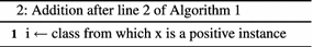
  • Following line is added after line 2:

    

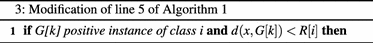
  • Line 5 of Algorithm 1 is modified as follows:

    

• 2. In the Gaussian ball B(x, e), centered at x with no false positive instance, we consider the e distance as the distance between x and the $j^{th}$ nearest neighbor instead of the first nearest neighbor. j is determined empirically, so that $|G|< j < 1$.This step aims to enlarge $x \cdot radius$ in the Adjusted-distance equation and, consequently, to expand the decision boundary. Line 9 in Algorithm 1 becomes:

The modified approach is denoted as MkRENN for future reference.

6 Experiments and result

6.1 Dataset

To test the proposed methodology, we tried to select a dataset as close as possible to the dataset used in the study that this current work improves. For this, we chose Aruba and Tulum real-world datasets collected from CASAS smart homes (CASAS Project 2007), a project of Washington State University. Data collected from Aruba dataset was obtained using 31 motion sensors, three door sensors, five temperature sensors, and three light sensors. 11 activities were performed for 220 days (7 months). Regarding Tulum dataset, data from 19 sensors were collected. 10 activities were performed for 83 days (4 months) by two residents. These data are all represented as a sequence of time-stamped sensor data, as shown in Fig. 2. The two datasets are imbalanced, as some of the activities occur more frequently than others.

Table 1 Statistics of the used datasets

Left part of Table 1 presents the statistics of the sensor events and activities performed in the Aruba dataset. “Other activity” class contains events with missing labels. It covers 54 % of the entire sensors events sequence. Due to the very large quantity of data to process with a normal computer (4 cores processor at 1.5 GHz machine with 8GB RAM—parallel execution was done on the 4 cores), we used only the first six weeks of data in Aruba dataset and 3 months of data in Tulum dataset.

Evaluation metrics used in this paper are classification accuracy and F-measure (F-score). The accuracy shows the percentage of correctly classified instances; while the average percentage of correctly classified instances per class is shown by the F-measure. It is favored over accuracy when we have an imbalanced dataset (as accuracy may be altered by correct classification of the most important class in the dataset).

6.2 Results and discussion

We conducted two sets of experiments to evaluate the effectiveness of the approaches presented in this paper. In the first series of experiments, the system was trained on data excluding “other activity” class. This class is incorporated in the second set of experiments to evaluate the system in a real environment situation. In the two sets of experiments, the four feature extraction methods described in Sect. 4, and five different classifiers (traditional SVM, traditional KNN, CB-kNN, MkENN and MkRENN) are evaluated. For SVM, we used the LibSVM (Chang and Lin 2011) library, with a penalty parameter (C) fixed to the value of 100 (empirically chosen) and an RBF kernel with the value of the variance of the kernel determined via cross-validation on the training data.

6.2.1 Learning on data excluding the “other” activity

We begin our experiment by testing Baseline features extraction method with different number of events per window. We obtained the best performances (classification) with 10 events per window. This number is lower than the average number of sensor events that span the duration of the different activities that is 70. Once the number of events per window is determined, we test the remaining features extraction methods. The experimental results obtained by the different features extraction and classification methods are summarized in Table 2. From the table, we can conclude two things about the different classifiers used. The first conclusion is that our modified algorithm of k Exemplar Nearest Neighbors technique (MkRENN) outperforms all KNN techniques. A second conclusion is that this presented approach (MkRENN) is comparable with traditional SVM classifier. When used in conjunction with the features extraction methods SWMIex and SWLS, MkRENN achieves almost the same results as SVM classifier.

Table 2 Results of the different classification algorithms without considering “Other activity” class

Table 3 Results of the different classification algorithms considering “Other activity” class

On Aruba dataset, the accuracy obtained by SVM for all the classes are close to each other, while there is a significant improvement in F-measure when using our features extraction method compared to the Baseline method. That can be explained by the fact that Aruba dataset is a very imbalanced dataset where half of the activities have too few data. F-measure is sensitive to any improvement in performance of these activities while accuracy is less sensitive to it. KNN classifiers results show a noticeable increase of 2 % in accuracy when our features extraction methods (SWMIex and SWLS) are used. On Tulum dataset, our features extraction methods outperform clearly Baseline and SWMI (Krishnan and Cook 2014) methods whatever the classifier used in the next stage.

Figure 8a, b shows the F-measure of each activity obtained by SVM classifier. Some of the activities (“Resperate” (8) and “Wash_Dishes” (10) from the Aruba dataset, “R2_eat_breakfast” (8) and “Wash_dishes” (10) for Tulum dataset) are identified only when the two presented extraction methods SWMIex and SWLS are used.

We decided to use KNN-based methods because they do not require a training phase and because they have the ability to identify the minority class as described in Sect. 4. In this set of experiment, the “other activity” class that covers over 54 % of the Aruba dataset is excluded and SVM training phase spins in an acceptable time. The interest of using KNN-based will appear in the second set of experiment.

6.2.2 Learning on data containing “other activity” class

To evaluate the system in a real situation, “other activity” class is now kept in the dataset. The results are summarized in Table 3. The classification accuracy is defined by:

$$\begin{aligned} Accuracy = \sum _{m=1}^{nb_A} \frac{TP_{A_M}}{N_{A_M}} \end{aligned}$$

(6)

Such that $nb_A$ is the total number of activities excluding the “other activity”.

By comparing the results obtained in the first series of experiments (Table 2) with the one obtained by this series (Table 3), classification accuracy drops significantly from 87 to 69 % in Aruba dataset. In Tulum dataset the performance degradation is more limited. This is due to the importance of “other activity” class in Aruba dataset, while this class is less present in Tulum dataset. Thus, the conclusions in the first set of experiment on Tulum dataset are still valid for this set of experiment.

From Table 3, we can conclude that MkRENN classifier outperforms all KNN classifiers. In addition, it remains comparable with traditional SVM. It can even perform better (even if not statistically representative) than SVM as results on Aruba dataset show (Table 3: SWMI and SWMIex columns).

On Aruba dataset, our SWLS feature extraction method continues to outperform all the others, while our SWMIex method provides a better F-measure. We observe that SWMI approach loses its superiority over the Baseline.

Figure 9 shows that when the training is done with an SVM model, none of the feature extraction method is able to identify the “Resperate” and “Wash_Dishes” activities, due to the imbalanced problem intensified by the presence of “other activity” which dominates the dataset. We also observe that the system loses capability to recognize the “Housekeeping” activity, where most of the instances are classified as “other activity”. MkRENN show better results in identifying these activities. Figure 10 shows a comparison between individual activities F-measure obtained by SVM and MkRENN classifiers both following feature extraction by SWMIex method.

Fig. 8

SVM classification on both datasets. Individual activities F-measure for different features extraction methods when “other” activity is excluded from dataset

Fig. 9

Aruba dataset. Individual activities F-measure for different features extraction methods when “other” activity is included

Table 4 CPU time of each classifiers when learning with the “other activity” class

Fig. 10

Aruba dataset. Individual activities F-measure for SVM and MkRENN classifiers when “other” activity is included

What we gained mostly in this set of experiment is classification performance that is close or better than the ones obtained by SVM without going through the learning phase. To clarify this point, Table 4 provides CPU Time consumption of this set of experiments. These measures have been done using a computer with an 1.5 GHz processor and 8GB RAM. KNN implementation used are Matlab (MathWorks, Natick, Massachusetts, US) codes and the SVM used are from LibSVM loaded from Matlab using a Mex-file. For these experiments, the computing time for the resolution of the whole training or testing set has been measured and to obtain the computing time for one sample, this batch time is divided by the number of samples in the set.

Although the part of the dataset that we used in this paper represents only 20 % of the whole, SVM classifiers took three days to learn the activity models. To train the entire dataset with SVM, it requires 23 days (with an optimized algorithm using parallel computing capacity of the computer.

It is obvious that SVM becomes unfeasible when the size of the available data is large (except if we do not want to specialize or to update the model, in that case one training is needed for every home and that is it). As in many applications more training data leads to better classifier, we cannot be limited in this part. The test phase in SVM is fast since it depends on the support vectors that are fewer than the training instances and since it does need only to project the new data in the kernel space and to compute a distance to the margin). As there is no model to build in KNN and its variants, the test phase depends on the size of training set and on the capacity of the algorithm to determine quickly the neighbors without having to go through the entire dataset. It is a costly phase in term of time and memory in case of huge dataset. In our situation even when working with the entire dataset, KNN techniques are more suitable than SVM.

7 Conclusion and future work

In order to provide an automated monitoring system for different human needs, an online system that performs activity recognition from sensor readings is required. Most of the techniques used in the literature are not suitable to build an online system. In this paper we propose and evaluate an extension of a sensor window approach to perform activity recognition in an online/streaming setting; recognizing activities when a new sensor event is recorded.

As different activities can be better characterized using different window length, mutual information based weighting of sensor events within a window is incorporated in this paper. A modification of how the mutual information is computed is proposed in this paper. To account for the fact that some sensors have different cone sizes (small, medium, large) we propose a last-state of sensor feature set within the window to characterize activities. For the classification part of our methodology, we proposed a Multi-classes Exemplar-based Nearest Neighbors (MkRENN) classifier to overcome the high computational cost of the SVM training phase.

These techniques were evaluated on Aruba datasets over six weeks and on Tulum dataset over 3 months.

The results show that the proposed MkRENN classifier could outperform SVM without the need to learn a model for each activity. In the feature extraction techniques, there was an improvement over the Baseline technique when any events with missing labels were removed (the “other activity” class). Only one of these techniques shows a significant improvement over Baseline when we incorporate events with missing indexation in the data. Indeed, there are a large confusion between “other activity” class and the different known activities. Our future work will include finding a way to reduce confusion between this activity and the others.

References

Bao L, Intille SS (2004) Activity recognition from user-annotated acceleration data. In: Pervasive computing: second international conference (PERVASIVE 2004), Linz/Vienna, Austria, April 21–23, Springer
Blanzieri E, Melgani F (2008) Nearest neighbor classification of remote sensing images with the maximal margin principle. IEEE Trans Geosci Remote Sens 46(6):1804–1811
CASAS Project (2007) Aruba, tulum datasets from wsu casas smart home project. http://ailab.wsu.edu/casas/datasets/
Chang CC, Lin CJ (2011) LIBSVM: a library for support vector machines. ACM Trans Intell Syst Technol (TIST) 2(3):Art. num. 27
Collobert R, Bengio S, Bengio Y (2002) A parallel mixture of SVMs for very large scale problems. Neural Comput 14(5):1105–1114
Cook D, Schmitter-Edgecombe M, Crandall A, Sanders C, Thomas B (2009) Collecting and disseminating smart home sensor data in the casas project. In: Proceedings of the 27th international conference on human factors in computing systems, CHI 2009, Boston, MA, USA, April 4–9
Domeniconi C, Gunopulos D (2001) Incremental support vector machine construction. In: Data mining, 2001. ICDM 2001, Proceedings IEEE international conference on, IEEE, pp 589–592
Gu T, Wu Z, Tao X, Pung HK, Lu J (2009) epSICAR: An emerging patterns based approach to sequential, interleaved and concurrent activity recognition. In: Pervasive computing and communications, 2009. PerCom 2009. IEEE international conference on, pp 1–9. doi:10.1109/PERCOM.2009.4912776
Intille SS, Larson K, Tapia EM, Beaudin JS, Kaushik P, Nawyn J, Rockinson R (2006) Using a live-in laboratory for ubiquitous computing research. In: Proceedings of the 4th international conference on pervasive computing, Springer, PERVASIVE’06, pp 349–365
Krishnan NC, Cook DJ (2014) Activity recognition on streaming sensor data. Pervasive Mob Comput 10:138–154
Li B, Chen YW, Chen YQ (2008) The nearest neighbor algorithm of local probability centers. IEEE Trans Syst Man Cybern Part B (Cybernetics) 38(1):141–154
Li Y, Zhang X (2011) Improving K nearest neighbor with exemplar generalization for imbalanced classification. In: Proceedings of the 15th Pacific-Asia conference on advances in knowledge discovery and data mining (PAKDD’11)—volume Part II, Springer, pp 321–332
Ni KS, Nguyen TQ (2009) An adaptable-nearest neighbors algorithm for mmse image interpolation. IEEE Trans Image Process 18(9):1976–1987
Poggio T, Cauwenberghs G (2001) Incremental and decremental support vector machine learning. Adv Neural Inf Process Syst 13:409
Pollack ME, Brown L, Colbry D, McCarthy CE, Orosz C, Peintner B, Ramakrishnan S, Tsamardinos I (2003) Autominder: an intelligent cognitive orthotic system for people with memory impairment. Robot Auton Syst 44(3):273–282
Pronobis A, Jie L, Caputo B (2010) The more you learn, the less you store: memory-controlled incremental svm for visual place recognition. Image Vis Comput 28(7):1080–1097
Syed NA, Huan S, Kah L, Sung K (1999) Incremental learning with support vector machines. In: Workshop on support vector machines at the international joint conference on artificial inteligence (IJCAI’99)
Tapia EM, Intille SS, Larson K (2004) Activity recognition in the home using simple and ubiquitous sensors. In: International conference on pervasive computing, Springer, pp 158–175
Voulgaris Z, Magoulas GD (2008) Extensions of the K nearest neighbour methods for classification problems. In: The 26th IASTED conference on artificial intelligence and applications, pp 23–28
Wang L, Gu T, Tao X, Lu J (2012) A hierarchical approach to real-time activity recognition in body sensor networks. Pervasive Mob Comput 8(1):115–130
Yala N, Fergani B, Fleury A (2015) Feature extraction for human activity recognition on streaming data. In: 2015 international symposium on innovations in intelligent systems and applications (INISTA’2015), Madrid, Spain, Sept. 2–4, IEEE, pp 1–6
Author information
Authors and Affiliations
Corresponding author
Rights and permissions
About this article
Cite this article
Yala, N., Fergani, B. & Fleury, A. Towards improving feature extraction and classification for activity recognition on streaming data. J Ambient Intell Human Comput 8, 177–189 (2017). https://doi.org/10.1007/s12652-016-0412-1
Received:
Accepted:
Published:
Issue Date:
DOI: https://doi.org/10.1007/s12652-016-0412-1