
Abstract
The land-use/land-cover (LU/LC) information can be extracted through continuous monitoring and observation of the global environment in the field of RS and GIS (remote sensing and geographic information system). With many inventions on satellite technologies, RS plays a crucial role throughout the world, and the researchers had shown their interest in finding the past, present, and future LU/LC information using the RS satellite data. In this research work, the non-forest- and forest-covered changes of Javadi Hills located in India were simulated and predicted using the hybrid machine learning models. The Markov chain–artificial neural network with cellular automata (MC–ANN–CA) and Markov chain–logistic regression with cellular automata (MC–LR–CA) were used and compared using the actual LU/LC maps of 2009, 2012, and 2015 along with the spatial variables (slope, aspect, hill shade, and distance road map). The results of the comparative analysis between the predicted and actual map of 2015 had shown a higher percentage of correctness in the MC–ANN–CA model for the spatial variables like slope, aspect, and distance road map. The LU/LC for 2021 and 2027 was predicted using the MC–ANN–CA model. By 2021, the forest-covered area will decrease by nearly − 0.38%, and the non-forest-covered area will increase by 0.79%. By 2027, forest-covered areas will decrease by − 0.52%, and non-forest-covered areas will increase by 1.06%, respectively, indicating the impacts of human and urbanization on LU/LC in Javadi Hills.
Introduction
The surface of the earth consists of natural and artificial land cover. The natural surface includes grasslands, water bodies, barren lands, forest-covered areas, desert regions, hills, snow, and glaciers. The artificial surface includes build-up areas, agricultural farms, and artificial turf lands. Every living organism on earth depends on nature and its benefits. Human plays a crucial role in utilizing and protecting the LU/LC environment. On the other hand, humans also fail to protect the environment, and so, the LU/LC change happens across the globe (Heidarlou et al. 2019; Fonji and Taff 2014). Many environmentalists had shown their interest in mineral mapping, agricultural field analysis, and LU/LC classification using the spatial information (Sawant and Prabukumar 2018), and they had been worked effortlessly in monitoring the LU/LC changes that happened on the earth’s surface (El-Tantawi et al. 2019). For evaluating the LU/LC changes for the smaller areas, the RS scientist had used the field survey data and aerial images. Multispectral (MS) and hyperspectral (HS) satellite images were considered as an essential data source to model the past, present, and future LU/LC changes for the larger areas across the world (Fonji and Taff 2014; Thyagharajan and Vignesh 2019). MS and HS satellite images were analysed through the thorough process of pre-processing, classification, and by computing the LU/LC changes for different regions in the biosphere. Through the countless inventions of scientists, the RS data had been collected through different satellites and monitored continuously. Scientist uses the satellite data for research purposes, particularly in the field of RS. Size and resolutions will differ for every satellite data. The spatial RS databases used by the scientist for LU/LC classification and change detection are Indian Remote Sensing (IRS)–polar satellite (P3), IRS–P6, IKONOS, Landsat–MODIS, Thematic Mapper (TM), Enhanced Thematic Mapper (ETM), Linear Imaging and Self-Scanning Sensor (LISS)–III Advanced spaceborne thermal emission and reflection radiometer (ASTER), EO-1 (Hyperion Data), Airborne visible infrared imaging spectrometer (AVIRIS), SPOT5, Envisat, Polarimetric synthetic aperture radar (PoISAR), Synthetic aperture radar (SAR), Quickbird, and German aerospace centre (Thyagharajan and Vignesh 2019; Lu and Weng 2007).
Pre-processing was the initial process performed after the data acquisition. The reason behind this process was to enhance the quality and visibility of the acquired satellite image. Pre-processing methods include dereferencing, radiometric, atmospheric, geometric, and topographic correction. The purpose of this method was to remove the noise, cloud, and snow effects present in the satellite image (Thyagharajan and Vignesh 2019; Zhu 2017; Pandey et al. 2017; Lu and Weng 2007). The classification of pre-processed RS data was performed through the different phases like training sample selection, feature extraction, selecting appropriate classification algorithms, post-processing, and finally validating the classification performance through accuracy assessment. LU/LC classification methods are hard, soft (fuzzy), supervised, unsupervised, parametric, and nonparametric classifiers. All the categories of LU/LC classification methods are machine learning algorithms, and they compute the LU/LC change detection analysis through the help of LU/LC classified data. Genetic, evolutionary, swarm intelligence, and probabilistic reasoning algorithm was performed for LU/LC classification. The LU/LC classified multispectral images will provide a clear vision of the LU/LC changes in natural (grasslands, water bodies, barren lands, forest-covered areas, desert region, hills, snow, and glaciers) and artificial surface (build-up areas, agricultural farms, and artificial turf lands) of the earth (Thyagharajan and Vignesh 2019; Lu and Weng 2007; Ma et al. 2019; Aburas et al. 2019). Accuracy assessment was performed by validating the LU/LC classified image with the ground-truth referenced image. The ground-truth referenced data were accessed through field surveys using GPS (Global Positioning System), aerial or drone photography, Google Earth, and Google map images. The validation was performed by generating and comparing the random points (location) of the pixel in the LU/LC classified and the ground-truth referenced image (Chen et al. 2019; Tilahun and Teferie 2015; Mohajane et al. 2018; Rwanga and Ndambuki 2017; Bey et al. 2016).
Remote sensing and GIS are considered as the appropriate tools for LU/LC modelling. The LU/LC modelling helps in exploring the spatiotemporal LU/LC changes all around the world. The LU/LC modelling has been performed for many decades by researchers in the field of remote sensing, and the importance of LU/LC modelling is to identify the impact of human and other natural disasters on the environment. The LU/LC modelling provides necessary information for LU/LC planning. It helps the researchers to understand the driving force of LU/LC transformation and to predict the future cost-effective and ecological effects on the earth’s surface. The LU/LC modelling contributes significantly to biodiversity loss, deforestation, urban expansion, agricultural and crop damage, wetland change, and vegetation loss. The LU/LC modelling is necessary to know about the past, present, and future patterns of LU/LC changes for the particular area or location. By using the GIS techniques, the information of LU/LC modelling will be the scope of attention for the land resource planners, agriculturists, forest department, urban planners, and other government organizations (Bose and Chowdhury Bose and Chowdhury 2020; Tavangar et al. 2019). The dependent and independent variables are used for modelling the LU/LC change prediction for the particular area. The transition probability matrix that has been calculated for the LU/LC change classification map is considered as the dependent variable, and the factors which affect the cause of LU/LC changes are considered as the independent variables. The main problem is to predict the LU/LC change for a particular area with good accuracy. The algorithm used was more appropriate for researchers to predict the LU/LC changes. The independent variables are modelled and prepared through the distance metrics and it has been mainly used during the process of LU/LC change prediction (Anand and Oinam 2020; Behera NK and Behera 2020; Dinda et al. 2019; Mandal and Mondal 2019a, b; Reddy et al. 2017).
Predicting the future LU/LC change was performed by evaluating the relationship between the dependent (LU/LC change maps) and independent (slope, elevation, aspect, distance from the forest edge, road, water bodies, wasteland, grassland, agricultural land, and settlements) variables. The DEM (digital elevation model) spatial data were used for generating the slope, elevation, aspect, and other topographic maps. The shapefile of the distance variables (forest edge, road, water bodies, wasteland, grassland, agricultural land, and settlements) had extracted from the government organizations, forest management, land resource administrations, and Google Earth images. The LU/LC change information had helped the land resource management, forest department, and government officials in protecting the environment (Kumar et al. 2014; Kamwi 2018; Singh et al. 2015; Mishra and Rai 2016). Many RS researchers had applied different machine learning and data mining models for predicting the future LU/LC change by using the dependent and independent RS data. Some frequently used GIS predictive models are as follows: SLEUTH (slope, land use, exclusion, urban extent, transportation, and hill shade), state and transition simulation model (STSM), land transformation model (LTM), spatially explicit landscape event simulation (SELES), CLUE (conversion of land use and its effects), cellular automata (CA), Markov chain (MC), ANN (artificial neural network), logistic regression (LR), land change modeller (LCM), and GIS-based weights of evidence (WoE) approach. The main purpose of predicting the future LU/LC change was to provide useful information to the land resource planners, decision-makers, and government officials for taking an effective management plan in protecting the LU/LC environment (Yirsaw et al. 2017; Aburas et al. 2019; Bounouh et al. 2017).
In recent times, several RS researchers have focused on LU/LC modelling problem by computing the raw satellite images. LU/LC modelling has been an effective research problem in the field of remote sensing. The detailed process of LU/LC modelling represents the different phases like data acquisition, pre-processing, LU/LC classification, post-classification analysis, modelling the spatial variables, validation, and LU/LC change prediction (MohanRajan et al. 2020). The different distance metrics have been used for modelling the LU/LC changes for band selection, classification, clustering, and for modelling the spatial variables (Navin and Agilandeeswari 2020; Sawant and Prabukumar 2020). Tavares et al. (2019) had used Sentinel-1 and Sentinel-2 data to project the LU/LC classification map of Belem in the Eastern Amazon. LU/LC classification had performed using a machine learning RFC algorithm. The Sentinel-1 and Sentinel-2 datasets were used in the tropical regions since it provides good accuracy by using the RFC method. Kavzoglu (2017) had conducted an effective analysis of RFC with the OBIA (object-based image analysis) for the spectral and spatial information of Quickbird-2 data for Trabzon Province in Turkey. The two-tailed McNemar’s test had proved that the thematic information of object-based RFC was considerably good when comparing the accuracy of the object-based k-NN classification method. Adam et al. (2014) had used the RFC and support vector machine (SVM) for classifying the rapid eye multispectral satellite images of KwaZulu-Natal located in South Africa. The accuracy of the SVM classifier was lower than the RFC method. The McNemar’s test had proved that there was no significant difference in the confusion matrix of SVM and RFC method. Kantakumar and Neelamsetti (2015) had combined the parametric classifiers like MLC and ISODATA with the non-parametric decision tree classifier for assessing the LU/LC classes using multitemporal Landsat data during April and December 2013 of Sindhudurg district located at the state of Maharashtra, India. Taufik et al. (2019) used Landsat data for the year 2014 and calculated the NDVI and NDWI values. The unsupervised classifiers like fuzzy C-means (FCM), K-means, and ISODATA were used and compared. The performance of FCM attains good classification accuracy than K-means and the ISODATA method.
Navin and Agilandeeswari (2019) had used the Landsat and LISS-III satellite map for assessing the LU/LC change at Javadi Hills located in India. The results showed that the hybrid classification methodology of K-Means and MLC was robust, and the results were used for detecting the LU/LC change from 2009 to 2019. Haque and Basak (2017) had shown the LU/LC change from 1980 to 2010 in Tanguar Haor located in Sunamganj, Bangladesh, using Landsat time series data. The LU/LC change analysis was performed using pre-classification (NDVI (normalized difference vegetation index), NDWI (normalized difference water index), supervised maximum likelihood classifier (MLC), and change vector analysis (CVS)) and post-classification (image differencing, change dynamic analysis, aerial difference calculation, image rationing, and regression) approaches. Misra and Vethamony (2015) had evaluated the spatial and temporal LU/LC changes using Landsat and IRS-LISS-III satellite images for the years 1973, 1989, 2001, and 2011. Principal component analysis (PCA) was used to enhance the satellite image, and the hybrid (supervised and unsupervised) classification techniques were for assessing the landscape information for Mandovi–Zuari estuarine complex of Goa located in India. Elagouz et al. (2019) used Landsat satellite data to calculate the LU/LC change for the Egyptian Nile Delta from 1987 to 2015. LU/LC classification using unsupervised Iterative Self-Organizing Data Analysis (ISODATA) and supervised SVM classification methods had been performed. Khawaldah (2016) had used the hybrid classification model for classifying the Landsat data of Amman governorate, the capital city of Jordan, for the period of 1984 to 2014. The LU/LC classified map of 1999 and 2014 was validated and used for predicting the future LU/LC map of 2030 using the Markov model. Mansour et al. (2020) had predicted the LU/LC changes for the years 2028 and 2038 using the CA–MC model through the validation of actual Landsat images of 2008 and 2018 in the mountainous regions of Oman. Spatial variables (slope, aspect, and elevation) and parameters (population density, proximity to the road, and urban) were modelled and used during the simulation process. By using the Landsat data, Islam et al. (2018) used the MC, CA–MC, and ANN model to find the future LU/LC changes in Chunati Wildlife Sanctuary, Bangladesh. The significance of the driver variables like elevation, slope, and distance to the road had been assessed through the LR model. The result of ANN was found to be a good fit for predicting the LU/LC for the years 2020 and 2025. Saputra and Lee (2019) used the ANN-CA model for validating and predicting the LU/LC map of North Sumatra located in Indonesia for the years 2050 and 2070.
The spatial variables like altitude, distance from the road, aspect, soil type, and slope were used and compared to describe the performance of the ANN-CA model. The results of altitude and distance from the roads had shown a strong impact during the prediction process. Qiang and Lam (2015) applied the transition rules of the actual LU/LC map of 1996 and 2006 to simulate the LU/LC map of 2016. The transition rules of the ANN model were applied to the CA model to simulate the LU/LC changes in the Lower Mississippi River Basin located in south-eastern Louisiana, USA. Arsanjani et al. (2013) used the actual LU/LC maps of 2006 and 2016 to predict the future LU/LC map of 2026 for the Middle East region of Tehran (Iran), by using hybrid predictive models of LR MC and CA. Siddiqui et al. (2018) had analysed the time series satellite data for the years 1993, 2003, and 2013 to estimate the LU/LC changes in Lucknow located in India. The hybrid approach of LR-based CA–MC model had been used to analyse the landscape information for the year 2023. eSilva et al. (2020) validated the Landsat data of the semiarid river basin located in north-eastern Brazil during the years 1990, 1999, and 2002 to predict the LU/LC for the year 2035 using the ANN and MC simulation model. Munthali et al. (2020) used the CA–MC model for validating and predicting the LU/LC maps of the Dedza district in Malawi for the years 2025 and 2035. Huang et al. (2020) had combined the CA with the MC model to forecast the future LU/LC map of 2020 and 2030 in Beijing located in China. Ansari and Golabi (2019) had monitored and predicted the LU/LC map of 2030 in MeighanWetland located in Iran by using ANN and MC predictive models. Nurwanda and Honjo (2020) had used the hybrid model of multilayer perceptron (MLP) with MC to predict Indonesia’s Bogor city expansion and to find the LST (land surface temperature) for the year 2027. Poor et al. (2019) used the MLP neural network method to validate and simulate the forest loss from 2016 to 2050 in the region of Sumatran tiger landscape located in Indonesia.
The rest of the paper is given as follows: “Motivations and Contributions” section explains the motivation and contribution of this work. “Preliminary Concepts” section explains the preliminary concepts, and “Proposed Flow of LU/LC Prediction for Javadi Hills” section elaborates on the proposed methodology of this work. “Comparative Analysis” section explains the comparative analysis of the prediction method for the different study areas, and “Conclusion” section delivers the conclusion of this research work.
Motivations and Contributions
The detailed research and observation from many researchers on LU/LC change prediction for different regions around the world have helped us in understanding the importance of LU/LC change prediction analysis. Through the clarifications from many RS scientists in performing the LU/LC change prediction process, the real-time satellite images were collected through different satellite data providers around the world. The initial process after data collection was to provide good clarity and visibility to the acquired satellite images using pre-processing methods. Finding and representing the label for the pre-processed satellite image were calculated using a different classification algorithm. The LU/LC change detection between different periods must be properly validated and evaluated. Spatial variables should be carefully selected and validated for performing the LU/LC change prediction analysis for different periods. By using LU/LC change prediction algorithms, the predicted results are simulated and validated. The predicted LU/LC change results will assist the land resource management to take necessary actions in protecting nature and its atmosphere, if any changes had been observed in the study area. The main contributions of our work are as follows:
-
1.
LU/LC change was detected in the non-forest- and forest-covered region of Javadi Hills for the periods 2009 to 2012 and 2012 to 2015 using the result of the random forest classification method.
-
2.
MC–LR–CA and MC–ANN–CA predictive models were used and compared.
-
3.
In this work, we analysed and validated the spatial (environmental) variables like slope, aspect, hill shade, and distance road map with the dependent LU/LC map to provide good validation results during the prediction process for both the models (MC–LR–CA and MC–ANN–CA).
-
4.
From the comparative analysis, the results of the MC–ANN–CA model had shown a higher value than the MC–LR–CA model for the combinations of spatial variables like slope, aspect, and distance road map.
-
5.
The MC–ANN–CA model was successfully applied to forecast the non-forest- and forest-covered changes for the years 2021 and 2027.
-
6.
The changes that occurred in the non-forest- and forest-covered region of the Javadi Hills will assist land resource management and forest department to take appropriate actions for protecting the environment.
Preliminary Concepts
In this section, the concepts of LU/LC classification and prediction modelling were explained. For our research work, the LU/LC classification was performed using RFC and the LU/LC prediction using the combined machine learning models of MC–LR–CA and MC–ANN–CA. The concepts used for predicting the LU/LC changes in Javadi Hills are explained in “Random Forest Classifier” and “Artificial Neural Network” sections.
Random Forest Classifier
The ensemble learning RFC algorithm was used in digital image processing for classification and prediction. RFC forms the multiple decision trees through the subset of the training data, and each decision tree is formed by selecting the random samples from the training dataset. The features in the training datasets were selected by calculating the information gain, gain ratio, and Gini index.
Based on the voting or average results of each decision tree, the classification results were prepared and processed. Random forest classification was accurate and robust to noisy data and helps in executing the larger datasets efficiently (Jin et al. 2018; Pimple et al. 2017; Belgiu and Dragut 2016; Eisavi et al. 2015; Odindi et al. 2014). The working model of RFC is shown in Fig. 1.

Working flow of random forest classification for raster datasets
Cellular Automata-Markovian model
From the several studies on RS and GIS environment for LU/LC change prediction, we identified that the Markov chain and cellular automata are widely used for predicting the future LU/LC map. The Markov chain model represents the transition probability between the initial and the final state for determining the change among the LU/LC states. The random Markov chain process is discrete in both the time and state. The cellular automata is the discrete model that represents the nonlinear and spatially distributed system to provide the LU/LC patterns for the larger area. The cellular automata is the bottom-up dynamic model that helps in the spatial–temporal calculations. The cellular automata model is discrete in space–time and state and helps to simulate the time–space computations (Anand and Oinam 2020; Bose and Chowdhury 2020; Gupta and Sharma 2020; Satya et al. 2020; Somvanshi et al. 2020; Yatoo et al. 2020). Based on the transition probability matrix, the time-based changing aspects for the LU/LC classes are measured using the Markov chain model, while the spatial changing aspects among the LU/LC classes are measured by the cellular automata model (Mansour et al. 2020; Huang et al. 2020; Liping et al. 2018; Singh et al. 2018).
In Eqs. (1), (2), and (3), the \(Tm\) represents the transition probability matrix, \(P_{ij }\) is the probability from LU/LC class \(i\) to LU/LC class j; \(n\) is the number of land-use types; \(i,j\) is the land-use type of 1st and 2nd time periods; \(S\) is the LU/LC status at time; \(t\) and \(S\left( {t + 1} \right)\) is referred to as the time point.
Logistic Regression
LR is the machine learning model that helps in the predictive analysis of the data. LR is the binary classification problem used in the field of statistics. The dependent variables are binary (either 0 or 1), and the outcome is predicted based on the set of independent variables. LR aims to find the best fitting model for describing the relationship between the dependent and the group of independent variables. LR model can be represented in binary, multinomial, and ordinal forms (Das and Pandey 2019; Kale et al. 2016; Mandal and Mondal 2019a, b; Mondal and Mandal 2018). The dependent and independent variables were associated and assessed through the process of regression. In the field of remote sensing, the LR model had been used to forecast the LU/LC changes by using the relationship between the actual LU/LC change maps (dependent) and the spatial (independent) variables (Kumar et al. 2014; Islam et al. 2018; Arsanjani et al. 2013; Siddiqui et al. 2018). The probability of the binary value (either 0 = No change or 1 = change) in the LU/LC change map was considered as the dependent variable and it was defined by the logistic function in Eq. (4).
where \(P\left( c \right)\) represents the probability of the LU/LC change map (dependent variable), \({\text{EV}}\left( Y \right)\) represents the predictive value of the binary dependent variable \(Y\), \(\beta_{0}\) represents the estimated constant, and \(\beta_{n}\) is the estimated coefficient for each spatial variable \(X_{n}\). Equation (5) represents the transformed logistic function \(\left( P \right)\). From Eqs. (5) and (6), the linear representation of the logistic regression (LR) model was obtained and it was shown in Eq. (7).
Artificial Neural Network
The MLP or ANN was used as the LU/LC predictive modelling in the field of RS and GIS. The idea of ANN is made like a human brain where every neuron nodes carry the processing information between them. ANN with artificial neurons or processing units is interconnected by nodes. The input and output units comprise the processing units of ANN. As humans read rules and come up with a result, ANN also has some set of learning rules and come up with a result or output. Supervised and unsupervised learning methods are carried out during the training phase of the ANN. The initial phase of the ANN will recognize the data patterns visually and textually. The ANN works backward and adjusts the weight of the network connections until the actual and desired output produces the minimum error (Anand and Oinam 2020; Bose and Chowdhury 2020; Mandal and Mondal 2019a, b; Reddy et al. 2017).
The data were trained and analysed using the neural network model of the back-propagation learning algorithm. The non-linear relations were modelled using ANN with good accuracy during the pattern recognition, feature extraction, and land-cover classification. The three layers define the structure of the ANN model, and the layers are input, hidden, and output layer. The working flow of ANN for raster datasets is shown in Fig. 2. Each layer in the ANN model had been composed of user-defined inputs (neurons). The neurons in the input layer represent the dependent and independent variables. By using the input training samples, the output layer represents the classified classes. In the hidden layer, the computations of the neurons are performed through weights and the outputs are produced through the activation function (Islam et al. 2018; eSilva et al. 2020; Qiang and Lam 2015; Ansari and Golabi 2019; Nurwanda and Honjo 2020; Poor et al. 2019; Saputra and Lee 2019; Satya et al. 2020). Equation (8) provides the mathematical expression of the ANN model,
where \(w_{j}\) refers to the weights between input and hidden layer, \(x_{j }\) represents the user-defined inputs (neurons), Y represents the output layer, b refers to bias, and φ represents the activation function.
The resulting value of the ANN was determined by using the activation function. Equation (10) provides the mathematical expression of the sigmoid or activation function model. The output layer of classified classes was determined as either 0 or 1 using the values of the sigmoid function. The neurons of the input and the hidden layers are weighted randomly, and the maximum activation value was identified through the assigned probability of each pixel in the training data.

Working flow of artificial neural network for raster datasets
Proposed Flow of LU/LC Prediction for Javadi Hills
This research aims to classify and predict the LU/LC during 2021 and 2027 in the non-forest and forest covered regions of Javadi Hills. The flow of LU/LC prediction for the Javadi Hills is shown in Fig. 3. The following steps describe the flow of this research work.

Proposed flow of LU/LC prediction for Javadi Hills
-
i.
The IRS Satellite Resourcesat-1 LISS-III and Cartosat-1 DEM (digital elevation model) satellite images of Javadi Hills were acquired from National Remote Sensing Centre (NRSC), and ISRO (Indian Space Research Organization).
-
ii.
A layer stacking and ROI (region of interest) extraction was performed during the process of pre-processing.
-
iii.
The RFC method was used for classifying the enhanced or pre-processed satellite image.
-
iv.
The locations of the LU/LC classified classes were determined by using a random sampling method and it was compared with Google Earth reference data during the process of accuracy assessment.
-
v.
The non-forest and forest covered changes were considered as the dependent variable. The slope, aspect, hill shade, and the distance road map of Javadi Hills were considered as spatial variables. The dependent and independent variables were given as the input for the predictive models.
-
vi.
The spatial variables like slope, hill shade, aspect, and distance road map are validated with the dependent LU/LC map to provide good validation results during the prediction process for both the models (MC–LR–CA and MC–ANN–CA).
-
vii.
By using the best correctness predictive method, the results of LU/LC prediction were obtained.
The detailed analysis and implementation of the proposed flow of LU/LC prediction for the non-forest and forest covered region of Javadi Hills are described in the rest of the sessions.
Study Area and Data Acquisition
Our study falls across the non-forest and forest covered region of Javadi Hills spreads across the Tiruvannamalai and Vellore district located in Tamil Nadu, India. The Eastern Ghats of the Javadi Hills have been located near the ARF (Alangayam Reserved Forest). The LISS-III images (2009, 2012, and 2015) were collected from the Bhuvan Indian Geo-Platform of ISRO. The coordinates of our study area fall between 78.75E12.5 N and 79.0E12.75 N. The extracted LISS-III image for our study area is shown in Figs. 4, and 5. The ground image size of the acquired LISS-III data is 142 km *141 km.

Location of Javadi Hills, India—study area

Extracted LISS-III multispectral image for our study area (300*300): a 2009, b 2012, c 2015
The study area is shown in Fig. 4. The shapefile of the India map was extracted from DIVA-GIS (http://www.diva-gis.org/). It has prepared by using ArcGIS software. The Tamil Nadu map was extracted from the Bhuvan Indian Geo-Platform of ISRO (www.bhuvan.com), and the Javadi Hills location map was extracted from Google Earth Engine (https://www.google.com/earth/). Table 1 shows the characteristics and the source of the satellite images. The satellite data were processed with the UTM (Universal Transverse Mercator) GCS (geographic coordinate system)/WGS (World Geodetic System) 1984 (44 N) projection system.
Pre-processing
The raw satellite data should be enhanced using the process of pre-processing. Pre-processing has been used in every area mainly in the field of RS and GIS. The advantage of using this method will provide the enhancement to the raw satellite images (Thyagharajan and Vignesh 2019; Zhu 2017). In this research work, geometric corrections were made in the multispectral image for extracting the ROI coordinates of the Javadi Hills. Figure 6 represents the pre-processed LISS–III image of Javadi Hills for the time periods 2009, 2012, and 2015. The size of the pre-processed LISS-III image of Javadi Hills is 256 * 200 pixels.

Pre-processed LISS-III image of Javadi Hills (256 * 200): a 2009; b 2012; c 2015
The Workflow of LU/LC Classification and Change Prediction Process
In this study, RFC was used for classifying the LU/LC map of the Javadi Hills for the periods 2009, 2012, and 2015. To predict the LU/LC for the year 2021 and 2027, the MC–LR–CA and MC–ANN–CA models were used and compared.
Classification
The experimentation of LU/LC classification for the Javadi Hills was performed by the RFC model in QGIS open-source software using the R language. The needed libraries and packages were installed in R script for performing the LU/LC RF classification. The training data were stored as CSV (comma-separated values) file and it was converted to the shapefile. The shapefile was used as the training data. RFC is used to validate the training data by generating the decision trees from the subset of the random points in the training data. The results from the decision trees help in classifying the non-forest- and forest-covered regions of Javadi Hills. The LU/LC classification result is shown in Fig. 7.

Classified LU/LC maps of Javadi Hills for years a 2009, b 2012, c 2015
Modelling Spatial Variables
The spatial variables used for evaluating the LU/LC changes for Javadi Hills are slope, aspect, hill shade, and distance road map. The slope, elevation, and hill shade were prepared using the DEM datasets. The Cartosat-1 DEM of 30-m-spatial-resolution data was downloaded from the Bhuvan Indian Geo-Platform of Indian Space Research Organisation (http://bhuvan-noeda.nrsc.gov.in), and shapefiles of the distance road map of Javadi Hills are extracted from Google Earth Engine. The slope, aspect, and hill shade were prepared using the terrain analysis module in QGIS software, and the distance from the road map was prepared by using the Euclidean distance in ArcGIS software. The modelled spatial variable is shown in Fig. 8.

Spatial variables: a aspect, b slope, c hill shade, d distance road map
Predictive Analysis for Javadi Hills
Our work provides a clear view of the LU/LC change prediction using the MC–LR–CA and MC–ANN–CA predictive models. The systematic process of the predictive models was performed in MOLUSE (modules for land-use change simulations) module in QGIS software, and the overall procedure is described in the following steps.
-
Step 1: Define input data The inputs used for LU/LC modelling were the initial (2009) and final (2012) LU/LC classified maps along with the spatial variables (slope, aspect, hill shade, and distance road map) of Javadi Hills.

where I1 and I2 represent the initial and final LU/LC classified maps, and I3 to I7 represent the spatial variables, slope (I3), aspect (I4), hill shade (I5), and the distance road map (I6).
-
Step 2: Check geometry Check whether the geometric coordinates (GC) of all the input raster images were matched. If the geometric coordinates are matched, then go to Step 3; else, correct the geometric errors until it gets matched. Let GC represent the geometric coordinates of the input raster images.


where G [I1, I2] represents the geometric coordinates of the initial and final LU/LC classified maps and G [I3, I4, I5, I6] represent the geometric coordinates of the spatial variables.
-
Step 3: Compute transition probabilities The transition probability matrix was calculated using the MC model. The MC model provides the probability of LU/LC changes that happened from 2009 to 2012 for the non-forest- and forest-covered region of Javadi Hills. The results of the transition probability matrix were used for predicting the future LU/LC of the Javadi Hills. It computes every transition between LU/LC class F (forest) to LU/LC class NF (non-forest). The LU/LC change map (Cm) was produced and it was considered as a dependent variable.
where \(T\)(\({\text{I}}1\)) is the area (%) of the initial LU/LC classified map, \(T\) (\({\text{I}}2\)) is the area (%) of the final LU/LC classified map, \(Tm\) represents the Transition probability Matrix, and \(P_{{F,{\text{NF}}}}\) refers to the probability of change from LU/LC class \(F\) (forest) to LU/LC class \({\text{NF}}\) (non-forest) for the time periods \(T\)(\({\text{I}}1\)) and \(T\) (\({\text{I}}2\)).
-
Step 4: Transition potential modelling This step describes the relationship between the dependent and spatial variables. Every pixel on an image was modelled and trained using the predictive models (LR and ANN) separately. The working process of LR and ANN model is explained in “Logistic Regression” and “Artificial Neural Network” sections.
where Pa and Pl represent the ANN and LR model for training the dependent LU/LC change map (Cm) and independent spatial variables (I3, I4, I5, I6, and I7).
-
Step 5: CA simulation After transition potential modelling, the LU/LC simulation map is then modelled using the CA model. The pixels with the highest Tp (transition potential) and change in the current state were identified. The change of pixels from one class to another with subject to its neighbourhood was demonstrated using the CA model.
where S (T (Pa)) and S (T (Pa) +1) refer to the system status at different times t and t + 1 for the ANN model, S (T (Pl)) and S (T (Pl) +1) refer to the system status at different times t and t + 1 for the LR model, N is the cellular field, and F refers to the transition rule of the cellular state.
-
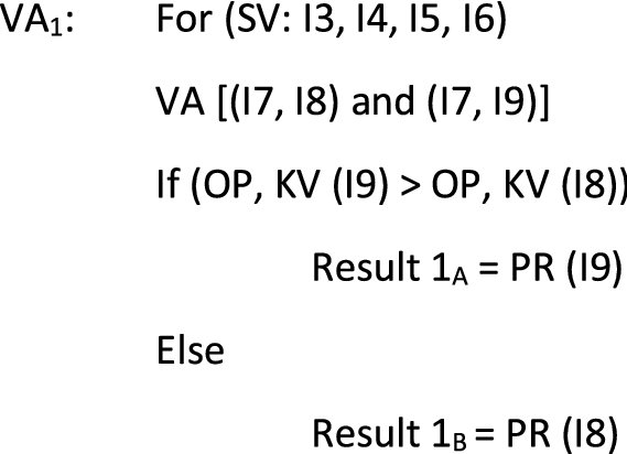
Step 6: Validation and prediction The results of the actual LU/LC classified map of 2015 (I7) were validated with the predicted LU/LC map of MA_LR_CA (I8) and MA_ANN_CA (I9) model. Both these prediction models were compared by computing the overall percentage of correctness (OP) and kappa value (KV) which is concisely described in “Validation of the Predicted Results” section. For the different combinations of spatial variables, all the validations (VA1 to VA5) were performed for both the predicted maps (I8 and I9) with the actual LU/LC map of 2015 (I7). The results of the predicted map are based on the evaluation of the overall percentage of correctness (OP) and kappa value (KV).
-
(i)
Validation 1 (VA1): With the combination of spatial variables I3, I4, I5, and I6, the first validation was performed for I7 with I8 and I9. If the overall percentage of correctness (OP) and kappa value (KV) I9 is greater than I8, then the predicted result of I9 is considered; else, the result of I8 is considered.
-
(ii)
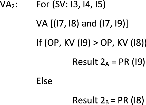
Validation 2 (VA2): With the combination of spatial variables I3, I4, and I5, the second validation was performed for I7 with I8 and I9. If the overall percentage of correctness (OP) and kappa value (KV) I9 is greater than I8, then the predicted result of I9 is considered; else, the result of I8 is considered.
-
(iii)
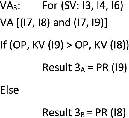
Validation 3 (VA3): With the combination of spatial variables I3, I4, and I6, the third validation was performed for I7 with I8 and I9. If the overall percentage of correctness (OP) and kappa value (KV) I9 is greater than I8, then the predicted result of I9 is considered; else, the result of I8 is considered.
-
(iv)
Validation 4 (VA4): With the combination of spatial variables I4, I5, and I6, the fourth validation was performed for I7 with I8 and I9. If the overall percentage of correctness (OP) and kappa value (KV) I9 is greater than I8, then the predicted result of I9 is considered; else, the result of I8 is considered.

-
(v)
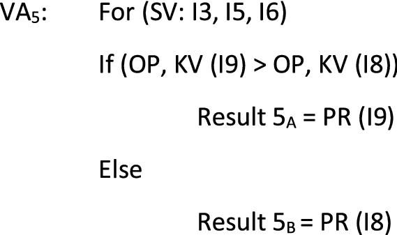
Validation 5(VA5): With the combination of spatial variables I3, I5, and I6, the fourth validation was performed for I7 with I8 and I9. If the overall percentage of correctness (OP) and kappa value (KV) I9 is greater than I8, then the predicted result of I9 is considered; else, the result of I8 is considered.


The validation was performed for the predicted map by using the combination of the spatial variables. We validated five different combinations of spatial variables (VA1 to VA5) with the predicted results (PR) of MA_LR_CA (I8) and MA_ANN_CA (I9) model. The validation results are shown in Tables 7 and 8. With the help of the validated results, the comparison between the MA_LR_CA and MA_ANN_CA model was made. After the validation (VA) and comparisons (CO), our results show a higher percentage of correctness in the MC–ANN–CA model for the spatial variables like slope, aspect, and distance road map. Our comparative results are shown in Table 9. With different combinations of spatial variables, the comparison was made for all five validations. The validated results that show the higher overall percentage of correctness and kappa value are considered.

Results and Discussion
This research work provides a complicated study of LU/LC prediction in Javadi Hills during the years 2021 and 2027. The LU/LC prediction in the non-forest- and forest-covered regions of the Javadi Hills had been conducted using LISS-III multispectral satellite images during 2009, 2012, and 2015. All experiments were conducted using R Studio, and geospatial processing software like ArcGIS, QGIS, and Google Earth Engine on Intel Xeon processor 2.90 GHz CPU along with 128 GB RAM in Windows 10 (64 bit) environment. The different statistical measurements were taken in this work for predicting the LU/LC change for the Javadi Hills.
Accuracy Assessment
The accuracy assessment results showed an overall accuracy along with user and producer accuracy by evaluating the Google Earth reference data with the classified data. We selected 356 random points (pixel location) from the LU/LC classified images of 2009, 2012, and 2015 and validated with the Google Earth images. The kappa statistics, and overall, user, and producer accuracies of individual LU/LC classes for non-forest- and forest-covered maps are presented in Table 2. An overall accuracy of 93.75% (kappa coefficient = 0.8644), 94.53% (kappa coefficient = 0.8813), and 95.70% (kappa coefficient = 0.8989) had been obtained for the year 2009, 2012, and 2015, respectively. The description of the classified LU/LC class is shown in Table 3.
Change Detection
The LU/LC classification results for the time series (2009, 2012, and 2015) data are presented in Table 4. In 2009, the LU/LC classified image was found to be 1622.5 ha (hectare) of the forest and 765.39 ha of non-forest. In 2012, the LU/LC classified image was found to be 1620.32 ha of the forest and 767.57 ha of non-forest. In 2015, the LU/LC classified image was found to be 1599.09 ha of the forest and 788.80 ha of non-forest.
The LU/LC change detection in Javadi Hills was performed between 2009 and 2012, 2012 and 2015, and 2009 and 2015. The changes in non-forest- and forest-covered regions of Javadi Hills were calculated and are shown in Table 5. The results showed a – 0.14% decrease in the forest area and 0.31% increase in the non-forest area during 2009 to 2012, − 1.27% decreases in the forest area and 2.72% increase in the non-forest area during 2012 to 2015, and − 1.42% decreases in the forest area and 3.04% increase in the non-forest area during 2009 to 2015.
The transition probabilities matrix was calculated using the MC analysis for the period of 2009 to 2015. The change results were analysed and used during the LU/LC change prediction. The transition probability matrix was calculated and is tabulated in Table 6.
Validation of the Predicted Results
From the results of the MC–LR–CA and MC–ANN–CA model, the predicted LU/LC map of 2015 is validated with the actual classified LU/LC map of 2015. The validated result of the predicted map analysis using the MC–LR–CA model from the five different combinations of variables is presented in Table 7 and MC–ANN–CA model is presented in Table 8. To determine the predicted map using the four spatial variables, many simulations were conducted by using each criterion with combinations of other variables.
As displayed in Tables 7 and 8, the overall percentage of correctness and kappa values looks good when validating the classified LU/LC map of 2015 with the predicted LU/LC map of 2015. Among these values, the combination of spatial data with slope, aspect, and distance road map produced the highest percentage of correctness in both the predicted models (MC–LR–CA and MC–ANN–CA). The results for MC–LR–CA model produced the highest percentage of correctness of 92.79% and the kappa value of 0.83. The results for the ANN-CA model produced the highest percentage of correctness of 93.68% and the kappa value of 0.85. From our analysis, we have found that the combination of spatial variables like slope, aspect, and distance road map provides the good validation results than other combinations for both the predicted models (MC–LR–CA and MC–ANN–CA).
From the validated results, we have compared the results of MC–LR–CA and MC–ANN–CA using the best combination of spatial variables like slope, aspect, and distance road map. The validated results are presented in Table 9. The results showed that the correctness of the MC–ANN–CA model is higher than the result of the MC–LR–CA model. Figure 9 shows the predicted and classified map of 2015. The result of the MC–ANN–CA model was applied to forecast the LU/LC changes for 2021 and 2027.

Classified and predicted LU/LC map 2015; a classified LU/LC map 2015, b predicted LU/LC map 2015
Correlation Analysis of Spatial Variables
The combinations of spatial variables like slope, aspect, and distance road map provide good validation results. The correlation analysis of slope, aspect, and a distance road map was computed and is shown in Table 10. The result showed that there exist correlation coefficients between 0.0363 and 0.4737. A high correlation happened between the slope and distance road map. The lowest coefficients occurred between the slope and the aspect.
Growth Pattern of the Future LU/LC
The present research is based on the integration of MC–ANN–CA and MC–LR–CA. From the deep analysis and validation, the MC–ANN–CA model provides a higher percentage of correctness than the MC–LR–CA model for the combination of spatial variables (slope, aspect, and distance road map). The MC–ANN–CA model was used to predict the LU/LC changes for 2021 and 2027. The predicted LU/LC map is shown in Fig. 10. The area statistics of the predicted map was calculated and is tabulated in Table 11. In 2021, the LU/LC for Javadi Hills was found to be 1593.06 ha of forest and 794.83 ha of non-forest. In 2027, the LU/LC for Javadi Hills was found to be 1591.08 ha of forest and 796.81 ha of non-forest.

Predicted LU/LC maps for years a 2021, b 2027
The LU/LC change prediction in the Javadi Hills was performed between 2015 and 2027. The predicted percentage of changes in non-forest- and forest-covered regions of Javadi Hills was evaluated and is shown in Table 12. The results showed a – 0.38% decrease in the forest area and 0.79% increase in the non-forest area during 2015 to 2021, − 0.13% decreases in the forest area and 0.27% increase in the non-forest area during 2021 to 2027, and − 0.52% decreases in the forest area and 1.06% increase in the non-forest area during 2015 to 2027.
Comparative Analysis
To justify the performance of the proposed LU/LC predication method for the combination of spatial variables, the other similar conventional methods are compared with the dataset of our study location. The comparitive analysis of LU/LC prediction methods for the five different study areas in India using the various combinations of spatial variables has been carried out and it is shown in Table 13. Based on the combination of spatial variables, the authors have predicted and validated the results for their study areas. We infer that the prediction results have been varying for the different study areas. The performance of our proposed method has given a higher overall percentage of correctness. The combination of spatial variables varies according to the study area, and it has been considered to be important for our method to validate and predict the LU/LC map.
Conclusion
Modelling the LU/LC changes and predicting the LU/LC information were considered as the essential focus in the area of RS and GIS. The LISS–III satellite data of Javadi Hills during the periods 2009, 2012, and 2015 were used for predicting the non-forest and forest covered region for the years 2021 and 2027. The layer stacking and geometric corrections were used for pre-processing the extracted satellite image. The RFC method was used for classifying the non-forest and forest covered regions of the Javadi Hills. The overall classification accuracy obtained during the years 2009, 2012, and 2015 are 93.75%, 94.53%, and 95.70% respectively. Our results show that – 0.14% decrease in the forest area and 0.31% increase in the non-forest area during 2009 to 2012, − 1.27% decreases in the forest area and 2.72% increase in the non-forest area during 2012 to 2015, and − 1.42% decreases in the forest area and 3.04% increase in the non-forest area during 2009 to 2015. The slope, aspect, hill shade, and distance road map were used as spatial variables for training the prediction models. The correlation analysis of spatial variables is also calculated, and the result shows a high correlation between the slope and distance road map and the lowest coefficients between the slope and the aspect. This paper presents a hybrid machine learning technique (MC–LR–CA and MC–ANN–CA) for predicting the non-forest and forest covered change in the Javadi Hills. From the different combinations of spatial variables, the slope, aspect, and distance road map had shown a good impact during the validation process for both the machine learning techniques (MC–LR–CA and MC–ANN–CA). From comparative analysis, the spatial variables (slope, aspect, and distance road map) of the MC–ANN–CA model provide a higher percentage of correctness (93.68%) and kappa value (0.85) than the MC–LR–CA model. Then, the results of the MC–ANN–CA model were used to predict the LU/LC changes for the years 2021 and 2027. The predicted results shows that there will be a – 0.38% decrease in the forest area and 0.79% increase in the non-forest area during 2015 to 2021, − 0.13% decreases in the forest area and 0.27% increase in the non-forest area during 2021 to 2027, and − 0.52% decreases in the forest area and 1.06% increase in the non-forest area during 2015 to 2027. The comparative analysis of the LU/LC prediction method for the different study areas using the various combinations of spatial variables has also been explained. From the comparative analysis of prediction methods for the different study areas, we infer that the performance of our proposed method has given a higher overall percentage of correctness. The findings of this research provides information to the land resource planners, policy-makers, government officials, and forest departments, to take action in protecting the land resource, mainly the forest-covered region from deforestation. Eventhough the validation and prediction time is more, the prediction method is resource-intensive. The future scope of this method is to improve the prediction accuracy by including the additional spatiotemporal variables like distance from the forest edge, settlements, and water body’s, soil type, census, and climatic data.
References
Aburas, M. M., Ahamad, M. S. S., & Omar, N. Q. (2019). Spatio-temporal simulation and prediction of land-use change using conventional and machine learning models: a review. Environmental Monitoring and Assessment, 191(4), 205. https://doi.org/10.1007/s10661-019-7330-6.
Adam, E., et al. (2014). Land-use/cover classification in a heterogeneous coastal landscape using RapidEye imagery: Evaluating the performance of random forest and support vector machines classifiers. International Journal of Remote Sensing, 35(10), 3440–3458. https://doi.org/10.1080/01431161.2014.903435.
Anand, V., & Oinam, B. (2020). Future land use land cover prediction with special emphasis on urbanization and wetlands. Remote Sensing Letters, 11(3), 225–234. https://doi.org/10.1080/2150704X.2019.1704304.
Ansari, A., & Golabi, M. H. (2019). Prediction of spatial land use changes based on LCM in a GIS environment for Desert Wetlands–A case study: Meighan Wetland, Iran. International Soil and Water Conservation Research, 7(1), 64–70. https://doi.org/10.1016/j.iswcr.2018.10.001.
Arsanjani, J. J., et al. (2013). Integration of logistic regression, Markov chain and cellular automata models to simulate urban expansion. International Journal of Applied Earth Observation and Geoinformation, 21, 265–275. https://doi.org/10.1016/j.jag.2011.12.014.
Behera, N. K., & Behera, M. D. (2020). Predicting land use and land cover scenario in Indian national river basin: The Ganga. Tropical Ecology. https://doi.org/10.1007/s42965-020-00073-x.
Belgiu, M., & Dragut, L. (2016). Random forest in remote sensing: A review of applications and future directions. ISPRS Journal of Photogrammetry and Remote Sensing, 114, 24–31. https://doi.org/10.1016/j.isprsjprs.2016.01.011.
Bey, A., et al. (2016). Collect earth: Land use and land cover assessment through augmented visual interpretation. Remote Sensing, 8(10), 807. https://doi.org/10.3390/rs8100807.
Bose, A., & Chowdhury, I. R. (2020). Monitoring and modeling of spatio-temporal urban expansion and land-use/land-cover change using markov chain model: A case study in Siliguri Metropolitan area, West Bengal, India. Modeling Earth Systems and Environment, pp. 1–15.
Bounouh, O., Essid, H., & Farah, I.R. (2017). Prediction of land use/land cover change methods: A study. In 2017 international conference on advanced technologies for signal and image processing (ATSIP) (pp. 1–7). IEEE. https://doi.org/10.1109/ATSIP.2017.8075511.
Chen, L., et al. (2019). Remote Sensing for Detecting Changes of Land Use in Taipei City, Taiwan. Journal of the Indian Society of Remote Sensing, 47(11), 1847–1856. https://doi.org/10.1007/s12524-019-01031-4.
Das, P., & Pandey, V. (2019). Use of Logistic Regression in Land-Cover Classification with Moderate-Resolution Multispectral Data. Journal of the Indian Society of Remote Sensing, 47(8), 1443–1454. https://doi.org/10.1007/s12524-019-00986-8.
Dinda, S., et al. (2019). Integration of GIS and statistical approach in mapping of urban sprawl and predicting future growth in Midnapore town. India. Modeling Earth Systems and Environment, 5(1), 331–352. https://doi.org/10.1007/s40808-018-0536-8.
Eisavi, V., et al. (2015). Land cover mapping based on random forest classification of multitemporal spectral and thermal images. Environmental Monitoring and Assessment, 187(5), 291. https://doi.org/10.1007/s10661-015-4489-3.
Elagouz, M. H., et al. (2019). Detection of land use/cover change in Egyptian Nile Delta using remote sensing. The Egyptian Journal of Remote Sensing and Space Science. https://doi.org/10.1016/j.ejrs.2018.10.004.
El-Tantawi, A. M., et al. (2019). Monitoring and predicting land use/cover changes in the Aksu-Tarim River Basin, Xinjiang-China (1990–2030). Environmental Monitoring and Assessment, 191(8), 480. https://doi.org/10.1007/s10661-019-7478-0.
eSilva, L. P., et al. (2020). Modeling land cover change based on an artificial neural network for a semiarid river basin in northeastern Brazil. Global Ecology and Conservation, 21, e00811. https://doi.org/10.1016/j.gecco.2019.e00811.
Fonji, S. F., & Taff, G. N. (2014). Using satellite data to monitor land-use land-cover change in North-eastern Latvia. Springerplus, 3(1), 61. https://doi.org/10.1186/2193-1801-3-61.
Gupta, R., & Sharma, L. K. (2020). Efficacy of Spatial Land Change Modeler as a forecasting indicator for anthropogenic change dynamics over five decades: A case study of Shoolpaneshwar Wildlife Sanctuary, Gujarat. India. Ecological Indicators, 112, 106171. https://doi.org/10.1016/j.ecolind.2020.106171.
Haque, M. I., & Basak, R. (2017). Land cover change detection using GIS and remote sensing techniques: A spatio-temporal study on Tanguar Haor, Sunamganj, Bangladesh. The Egyptian Journal of Remote Sensing and Space Science, 20(2), 251–263. https://doi.org/10.1016/j.ejrs.2016.12.003.
Heidarlou, H. B., et al. (2019). Effects of preservation policy on land use changes in Iranian Northern Zagros forests. Land use policy, 81, 76–90. https://doi.org/10.1016/j.landusepol.2018.10.036.
Huang, Y., et al. (2020). Analysis of the future land cover change in Beijing using CA–Markov chain model. Environmental Earth Sciences, 79(2), 60. https://doi.org/10.1007/s12665-019-8785-z.
Islam, K., Rahman, M. F., & Jashimuddin, M. (2018). Modeling land use change using cellular automata and artificial neural network: The case of Chunati Wildlife Sanctuary, Bangladesh. Ecological Indicators, 88, 439–453. https://doi.org/10.1016/j.ecolind.2018.01.047.
Jin, Y., et al. (2018). Land-cover mapping using Random Forest classification and incorporating NDVI time-series and texture: A case study of central Shandong. International Journal of Remote Sensing, 39(23), 8703–8723. https://doi.org/10.1080/01431161.2018.1490976.
Kale, M. P., et al. (2016). Land-use and land-cover change in Western Ghats of India. Environmental Monitoring and Assessment, 188(7), 387. https://doi.org/10.1007/s10661-016-5369-1.
Kamwi, J. M. (2018). Assessing the spatial drivers of land use and land cover change in the protected and communal areas of the Zambezi Region. Namibia. Land, 7(4), 131. https://doi.org/10.3390/land7040131.
Kantakumar, L. N., & Neelamsetti, P. (2015). Multi-temporal land use classification using hybrid approach. The Egyptian Journal of Remote Sensing and Space Science, 18(2), 289–295. https://doi.org/10.1016/j.ejrs.2015.09.003.
Kavzoglu, T. (2017). Object-oriented random forest for high resolution land cover mapping using quickbird-2 imagery. In Handbook of neural computation (pp. 607–619). Academic Press. https://doi.org/10.1016/B978-0-12-811318-9.00033-8.
Khawaldah, H. A. (2016). A prediction of future land use/land cover in Amman area using GIS-based Markov Model and remote sensing. Journal of Geographic Information System, 8(03), 412. https://doi.org/10.4236/jgis.2016.83035.
Kumar, R., et al. (2014). Forest cover dynamics analysis and prediction modeling using logistic regression model. Ecological Indicators, 45, 444–455. https://doi.org/10.1016/j.ecolind.2014.05.003.
Liping, C., Yujun, S., & Saeed, S. (2018). Monitoring and predicting land use and land cover changes using remote sensing and GIS techniques—A case study of a hilly area, Jiangle, China. PloS one, https://doi.org/10.1371/journal.pone.0200493.
Lu, D., & Weng, Q. (2007). A survey of image classification methods and techniques for improving classification performance. International Journal of Remote Sensing, 28(5), 823–870. https://doi.org/10.1080/01431160600746456.
Ma, L., et al. (2019). Deep learning in remote sensing applications: A meta-analysis and review. ISPRS Journal of Photogrammetry and Remote Sensing, 152, 166–177. https://doi.org/10.1016/j.isprsjprs.2019.04.015.
Mandal, S., & Mondal, S. (2019) Logistic regression (LR) model and landslide susceptibility: A RS and GIS-based approach. In Statistical approaches for landslide susceptibility assessment and prediction, Cham: Springer (pp. 107–121). https://doi.org/10.1007/978-3-319-93897-4_4.
Mandal, S., & Mondal, S. (2019). Artificial neural network (ann) model and landslide susceptibility. In Statistical approaches for landslide susceptibility assessment and prediction. Cham: Springer, (pp. 123-133). https://doi.org/10.1007/978-3-319-93897-4_5.
Mansour, S., Al-Belushi, M., & Al-Awadhi, T. (2020). Monitoring land use and land cover changes in the mountainous cities of Oman using GIS and CA-Markov modelling techniques. Land Use Policy, 91, 104414. https://doi.org/10.1016/j.landusepol.2019.104414.
Mishra, V. N., & Rai, P. K. (2016). A remote sensing aided multi-layer perceptron-Markov chain analysis for land use and land cover change prediction in Patna district (Bihar), India. Arabian Journal of Geosciences, 9(4), 249. https://doi.org/10.1007/s12517-015-2138-3.
Misra, A., & Vethamony, P. (2015). Assessment of the land use/land cover (LU/LC) and mangrove changes along the Mandovi-Zuari estuarine complex of Goa, India. Arabian Journal of Geosciences, 8(1), 267–279. https://doi.org/10.1007/s12517-013-1220-y.
Mohajane, M., et al. (2018). Land use/land cover (LULC) using Landsat data series (MSS, TM, ETM + and OLI) in Azrou Forest, in the Central Middle Atlas of Morocco. Environments, 5(12), 131. https://doi.org/10.3390/environments5120131.
MohanRajan, S. N., Loganathan, A., & Manoharan, P. (2020). Survey on land use/land cover (LU/LC) change analysis in remote sensing and GIS environment: Techniques and challenges. Environmental Science and Pollution Research, 27, 29900–29926. https://doi.org/10.1007/s11356-020-09091-7.
Mondal, S., & Mandal, S. (2018). RS & GIS-based landslide susceptibility mapping of the Balason River basin, Darjeeling Himalaya, using logistic regression (LR) model. Georisk: Assessment and Management of Risk for Engineered Systems and Geohazards 12(1), 29–44. https://doi.org/10.1080/17499518.2017.1347949.
Munthali, M. G., et al. (2020). Modelling land use and land cover dynamics of Dedza district of Malawi using hybrid Cellular Automata and Markov model. Remote Sensing Applications: Society and Environment, 17, 100276. https://doi.org/10.1016/j.rsase.2019.100276.
Navin, M. S., & Agilandeeswari, L. (2019). Land use land cover change detection using k-means clustering and maximum likelihood classification method in the Javadi Hills, Tamil Nadu, India. International Journal of Engineering and Advanced Technology (IJEAT). https://doi.org/10.35940/ijeat.A1011.1291S319.
Navin, M. S., & Agilandeeswari, L. (2020). Comprehensive review on land use/land cover change classification in remote sensing. Journal of Spectral Imaging. https://doi.org/10.1255/jsi.2020.a8.
Nurwanda, A., & Honjo, T. (2020). The prediction of city expansion and land surface temperature in Bogor City, Indonesia. Sustainable Cities and Society, 52, 101772. https://doi.org/10.1016/j.scs.2019.101772.
Odindi, J. O., et al. (2014). Comparison between WorldView-2 and SPOT-5 images in mapping the bracken fern using the random forest algorithm. Journal of Applied Remote Sensing, 8(1), 083527. https://doi.org/10.1117/1.JRS.8.083527.
Pandey, P., Dewangan, K. K., & Dewangan, D. K. (2017). Enhancing the quality of satellite images by preprocessing and contrast enhancement. In 2017 international conference on communication and signal processing (ICCSP) (pp. 0056–0060). IEEE. https://doi.org/10.1109/ICCSP.2017.8286525.
Pimple, U., et al. (2017). Topographic correction of Landsat TM-5 and Landsat OLI-8 imagery to improve the performance of forest classification in the mountainous terrain of Northeast Thailand. Sustainability, 9(2), 258. https://doi.org/10.3390/su9020258.
Poor, E. E., Shao, Y., & Kelly, M. J. (2019). Mapping and predicting forest loss in a Sumatran tiger landscape from 2002 to 2050. Journal of Environmental Management, 231, 397–404. https://doi.org/10.1016/j.jenvman.2018.10.065.
Qiang, Y., & Lam, N. S. (2015). Modeling land use and land cover changes in a vulnerable coastal region using artificial neural networks and cellular automata. Environmental Monitoring and Assessment, 187(3), 57. https://doi.org/10.1007/s10661-015-4298-8.
Reddy, C. S., et al. (2017). Predictive modelling of the spatial pattern of past and future forest cover changes in India. Journal of Earth System Science, 126(1), 8. https://doi.org/10.1007/s12040-016-0786-7.
Rwanga, S. S., & Ndambuki, J. M. (2017). Accuracy assessment of land use/land cover classification using remote sensing and GIS. International Journal of Geosciences, 8(04), 611. https://doi.org/10.4236/ijg.2017.84033.
Saputra, M. H., & Lee, H. S. (2019). Prediction of land use and land cover changes for North Sumatra, Indonesia, using an artificial-neural-network-based cellular automaton. Sustainability, 11(11), 3024. https://doi.org/10.3390/su11113024.
Satya, B. A., Shashi, M., & Deva, P. (2020). Future land use land cover scenario simulation using open source GIS for the city of Warangal, Telangana, India. Applied Geomatics. https://doi.org/10.1007/s12518-020-00298-4.
Sawant, S. S., & Prabukumar, M. (2018). A review on graph-based semi-supervised learning methods for hyperspectral image classification. The Egyptian Journal of Remote Sensing and Space Science. https://doi.org/10.1016/j.ejrs.2018.11.001.
Sawant, S. S., & Prabukumar, M. (2020). A survey of band selection techniques for hyperspectral image classification. Journal of Spectral Imaging. https://doi.org/10.1255/jsi.2020.a5.
Siddiqui, A., et al. (2018). Urban growth dynamics of an Indian metropolitan using CA Markov and Logistic Regression. The Egyptian Journal of Remote Sensing and Space Science, 21(3), 229–236. https://doi.org/10.1016/j.ejrs.2017.11.006.
Singh, S. K., et al. (2015). Predicting spatial and decadal LULC changes through cellular automata Markov chain models using earth observation datasets and geo-information. Environmental Processes, 2(1), 61–78. https://doi.org/10.1007/s40710-015-0062-x.
Singh, S. K., et al. (2018). Modelling of land use land cover change using earth observation data-sets of Tons River Basin, Madhya Pradesh, India. Geocarto international, 33(11), 1202–1222. https://doi.org/10.1080/10106049.2017.1343390.
Somvanshi, S. S., et al. (2020). Monitoring spatial LULC changes and its growth prediction based on statistical models and earth observation datasets of Gautam Budh Nagar, Uttar Pradesh, India. Environment, Development and Sustainability, 22(2), 1073–1091. https://doi.org/10.1007/s10668-018-0234-8.
Taufik, A., Ahmad, S. S. S., & Azmi, E. F. (2019). classification of landsat 8 satellite data using unsupervised methods. In Intelligent and interactive computing (pp. 275–284). Singapore: Springer. https://doi.org/10.1007/978-981-13-6031-2_46.
Tavangar, Sh, et al. (2019). A futuristic survey of the effects of LU/LC change on streamflow by CA–Markov model: A case of the Nekarood watershed, Iran. Geocarto International, 2019, 1–17. https://doi.org/10.1080/10106049.2019.1633419.
Tavares, P. A., et al. (2019). Integration of sentinel-1 and sentinel-2 for classification and LULC mapping in the urban area of Belém, eastern Brazilian Amazon. Sensors, 19(5), 1140. https://doi.org/10.3390/s19051140.
Thyagharajan, K. K., & Vignesh, T. (2019). Soft computing techniques for land use and land cover monitoring with multispectral remote sensing images: A review. Archives of Computational Methods in Engineering, 26(2), 275–301. https://doi.org/10.1007/s11831-017-9239-y.
Tilahun, A., & Teferie, B. (2015). Accuracy assessment of land use land cover classification using Google Earth. American Journal of Environmental Protection, 4(4), 193–198. https://doi.org/10.11648/j.ajep.20150404.14.
Yatoo, S. A., et al. (2020). Monitoring land use changes and its future prospects using cellular automata simulation and artificial neural network for Ahmedabad city, India. GeoJournal. https://doi.org/10.1007/s10708-020-10274-5.
Yirsaw, E. (2017). Land use/land cover change modeling and the prediction of subsequent changes in ecosystem service values in a coastal area of China, the Su-Xi-Chang Region. Sustainability, 9(7), 1204. https://doi.org/10.3390/su9071204.
Zhu, Z. (2017). Change detection using landsat time series: A review of frequencies, preprocessing, algorithms, and applications. ISPRS Journal of Photogrammetry and Remote Sensing, 130, 370–384. https://doi.org/10.1016/j.isprsjprs.2017.06.013.
Acknowledgements
Authors wish to thank Bhuvan Indian Geo-Platform of ISRO for freely providing the LISS–III data and Cartosat-1 DEM data for study area Javadi Hills, Tamil Nadu, India. We are thankful to the Google Earth Engine platform for providing the map of Javadi Hills. We wish to thank DIVA-GIS and ArcGIS geospatial software for preparing the shapefile of the India Map. We are thankful to the Vellore Institute of Technology for providing the VIT SEED GRANT for carrying out this work and CDMM (Centre for Disaster Mitigation & Management) for providing a good lab facility.
Author information
Authors and Affiliations
Corresponding author
Additional information
Publisher's Note
Springer Nature remains neutral with regard to jurisdictional claims in published maps and institutional affiliations.
About this article

Cite this article
MohanRajan, S.N., Loganathan, A. Modelling Spatial Drivers for LU/LC Change Prediction Using Hybrid Machine Learning Methods in Javadi Hills, Tamil Nadu, India. J Indian Soc Remote Sens 49, 913–934 (2021). https://doi.org/10.1007/s12524-020-01258-6
Received:
Accepted:
Published:
Issue Date:
DOI: https://doi.org/10.1007/s12524-020-01258-6