Inverse Mean Curvature Flow for Star-Shaped Hypersurfaces Evolving in a Cone

Abstract

For a given convex cone we consider hypersurfaces with boundary which are star-shaped with respect to the center of the cone and which meet the cone perpendicular. The evolution of those hypersurfaces inside the cone yields a nonlinear parabolic Neumann problem. We show that one can use the convexity of the cone to prove long time existence of this flow. Finally, we show that the hypersurfaces converge smoothly to a piece of the round sphere.

1 Introduction

The evolution of surfaces depending on their curvature has a long history, probably starting with the early work of Brakke [1]. A classical result for inverse mean curvature flow (IMCF) is due to Gerhardt [3]. He showed that starting from a closed, smooth, star-shaped hypersurface with strictly positive mean curvature, the surface evolves for all time and approaches a round sphere as time tends to infinity (see also Urbas [13]).

For non-star-shaped initial surfaces, singularities may occur in finite time. In order to make sense of the flow in that situation, Huisken and Ilmanen [4, 5] defined a notion of weak solutions to IMCF. This enabled them to prove the Riemannian Penrose inequality (see also Bray [2]).

In this work we want to consider classical solutions to IMCF in the case where the initial hypersurface is a star-shaped C ^2,α-surface with strictly positive mean curvature. In contrast to the work of Gerhardt, we will look at hypersurfaces which possess a boundary which meets the cone perpendicular. The cone can be seen as a supporting hypersurface for the evolving surface, and is not moving itself.

We prove that this flow will exist for all time, and the surfaces will converge to a piece of the round sphere. From the geometric point of view, a key step is an estimate for the slope of the height function, using the convexity of the cone. From an analytic point of view, a major step is to prove the full Schauder estimates without having direct access to a second derivative bound.

Let S ⁿ⊂ℝⁿ⁺¹ be the sphere of radius one. Let M ⁿ⊂S ⁿ be some piece of S ⁿ such that $\Sigma^{n} := \{ rx\in\mathbb{R}^{n+1} \; | \ r >0, \ x \in\partial M^{n} \}$ is the boundary of a smooth, convex¹ cone. We will prove the following theorem:²

Theorem 1

Let n≥2. Let Σⁿ⊂ℝⁿ⁺¹ be the boundary of a smooth, convex cone that is centered at the origin and has outward unit normal μ. Let F ₀:M ⁿ→ℝⁿ⁺¹ such that $M^{n}_{0}:=F_{0}(M^{n})$ is a compact C ^2,α-hypersurface which is star-shaped with respect to the center of the cone and has strictly positive mean curvature. Assume furthermore that $M^{n}_{0}$ meets Σⁿ orthogonally. That is,

where ν ₀ is the unit normal to $M^{n}_{0}$. Then there exists a unique embedding

with F(∂M ⁿ,t)⊂Σⁿ for t≥0, satisfying:

$$(\mbox{\textit{IMCF}})\begin{cases}\frac{\partial F}{\partial t} = \frac{\nu}{H}\circ F& \mbox{\textit{in}}\ M^n \times(0,\infty)\\\noalign{\vspace*{3pt}}\big\langle\mu\circ F, \nu\circ F\big\rangle= 0& \mbox{\textit{on}}\ \partial M^n \times(0, \infty) \\F(\, . \,,0) = F_0& \mbox{\textit{on}}\ M^n\end{cases}$$

where ν is the unit normal to $M^{n}_{t} := F(M^{n},t)$ pointing away from the center of the cone and H is the scalar mean curvature of $M^{n}_{t}$. The rescaled solution F(.,t)e ^−t/n converges smoothly to an embedding F _∞, mapping M ⁿ into a piece of a round sphere of radius $r_{\infty}= (|M^{n}_{0}|/|M^{n}|)^{1/n}$.

In the first part of the paper, we will prove short time existence and reduce (IMCF) to a scalar parabolic Neumann problem. The second part is concerned with a priori estimates for solutions to this problem, including the crucial bound of the slope of the height function. We show that the convexity of the cone can be used to control this quantity. The last part deals with the Hölder estimates which finally yield long time existence and convergence to a piece of the round sphere.

2 The Associated Neumann Problem

We want to describe the surface at time t as a graph over M ⁿ. Therefore, we make the ansatz

for some function u:M ⁿ×[0,T)→ℝ. Since the initial surface $M^{n}_{0}$ is a star-shaped C ^2,α-hypersurface, there exists a scalar function u ₀∈C ^2,α(M ⁿ) such that F ₀ can be expressed as F ₀:M ⁿ→ℝⁿ⁺¹:x↦u ₀(x)x. In order to work with graphs over M ⁿ, the following formulas are useful.

Lemma 1

Let t≥0 be fixed. Let $\tilde{M}^{n}_{t} := \tilde{F}(M^{n},t)$ and {σ _ij } _i,j=1,…,n denote the metric on M ⁿ. We define $p:=\tilde{F}(x,t)$ and assume that a point on M ⁿ is described by local coordinates, that is, x=x(ξ ⁱ). The following formulas hold:

• (i) Let $v:=\sqrt{1+u^{-2}|\nabla u|^{2}}$ and 1≤i≤n. Then the tangent vectors $\tau_{i} \in T_{p}\tilde{M}^{n}_{t}$ and the unit normal $\nu\in N_{p}\tilde{M}^{n}_{t}$ are given by

  

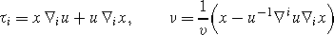
  where we used the same symbol for the position vector and the point x.

• (ii) The metric {g _ij } _i,j=1,…,n and inverse metric {g ^ij} _i,j=1,…,n on T $_{p}\tilde{M}^{n}_{t}$ are given by

  

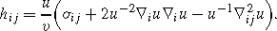
• (iii) The second fundamental form {h _ij } _i,j=1,…,n of $T_{p}\tilde{M}^{n}_{t}$ is given by

  

• (iv) Let p∈Σⁿ and $\hat{\mu}(p)$ be the normal to Σⁿ in p. Let μ=μ ^k(x)e _k (x) be the normal to Σⁿ in x and e _k the basis vectors of T _x S ⁿ. Then

  

The scalar mean curvature of $\tilde{M}^{n}_{t}$ is given by H=g ^ij h _ij . All derivatives are covariant derivatives with respect to the metric {σ _ij } _i,j=1,…,n on M ⁿ.

Proof

The formulas in (i) can be verified by direct calculation, and those in (ii) and (iii) are the same as in [3]. The equivalence in (iv) follows from the formula for ν and the fact that Σⁿ is a cone in ℝⁿ⁺¹ and therefore μ(rx)=μ(x). □

So far, $\tilde{F}$ only allows the evolution of points in radial direction. Since we want the surface to move in normal direction we modify the ansatz by defining

for some map φ:M ⁿ×[0,T)→M ⁿ which has to be bijective for fixed t and has to satisfy φ(∂M ⁿ,t)=∂M ⁿ. The problem of solving (IMCF) then reduces to solving

as is stated in the next lemma.

Lemma 2

Let F ₀ be as in Theorem 1. Then there exists some T>0, a unique solution u∈C ^2+α,1+α/2(M ⁿ×[0,T],ℝ)∩C ^∞(M ⁿ×(0,T],ℝ) of (∗), and a unique map φ:M ⁿ×[0,T]→M ⁿ such that the above-defined map F has the same regularity as stated in Theorem 1 and is the unique solution to (IMCF).

Proof

The conditions on F ₀ imply that u ₀ is a C ^2,α function which satisfies the compatibility condition ∇ _μ u ₀=0 on ∂M ⁿ. The inverse function theorem, together with the theory of linear parabolic Neumann problems, yields a unique solution to (∗). The higher regularity of u for t>0 can be proved by considering limits of difference quotients. Next, we choose φ to be the unique solution of the ordinary differential equation

The theory of ODE’s implies that φ is a diffeomorphism for fixed t and C ^1+α in t up to t=0. Note that the Neumann condition for u implies that φ(∂M ⁿ,t)=∂M ⁿ. Using Lemma 1, the equation for φ, and (∗), a direct calculation shows that F satisfies (IMCF). The uniqueness follows from the uniqueness of u and φ. □

Remark 1

The short time existence result also holds for immersed hypersurfaces in a Riemannian manifold and for arbitrary smooth supporting hypersurfaces Σⁿ (see [9]). The corresponding short time existence result for mean curvature flow was proved by Stahl [11].

Let T ^∗ be the maximal time such that there exists some u∈C ^2,1(M ⁿ×[0,T ^∗))∩C ^∞(M ⁿ×(0,T ^∗)) which solves (∗). In the following, we will prove a priori estimates for those admissible solutions on [0,T] where T<T ^∗.

3 Maximum Principle Estimates

Let u be an admissible solution of (∗). We define w:=lnu and observe that

Therefore, w solves

with

In contrast to the differential operator occurring in (∗), Q does not explicitly depend on the solution itself, but only on its first and second derivatives. In the following, we will use (∗∗) to derive estimates for |u|, |∂u/∂t|, |∇u|, and |H|. We define

Lemma 3

Let u be an admissible solution of (∗). Let Σⁿ be a smooth cone. Then u satisfies

Proof

Let w(x,t):=lnu(x,t) and $w^{+}(x,t) := \ln(\max_{M^{n}} u_{0} ) +t/n$. Using

with w _θ :=θw ⁺+(1−θ)w, we see that ψ:=w ⁺−w satisfies

The maximum principle implies ψ≥0 in M ⁿ×[0,T] and thus the upper bound. The lower bound is obtained using $w^{-}(x,t) := \ln(\min_{M^{n}} u_{0}) + t/n$. □

Remark 2

From a geometric point of view, this estimate says that the rescaled surfaces F(M ⁿ,t)e ^−t/n always stay between the two spherical caps which enclose the initial surface.

Next, we want to estimate |∂u/∂t|.

Lemma 4

Let u be an admissible solution of (∗). Let Σⁿ be a smooth cone. Then $\dot{u}:=\partial u/ \partial t$ satisfies

Here H ₀=H( . ,0), v=v( . ,0), and R ₁,R ₂ are the constants from Lemma 3.

Proof

Let $\dot{w}:=\partial w/\partial t$. Differentiating (∗∗) in the time direction leads to

The result follows from the maximum principle and the fact that $Q=\frac {v}{uH}$. □

For the estimate of |∇u|, we have to make use of the convexity of Σⁿ.

Lemma 5

Let u be an admissible solution of (∗). Let Σⁿ be a smooth, convex cone. Then ∇u satisfies

Proof

As in [3] we differentiate (∗∗) with respect to ∇ _k , multiply by ∇ _k w, and sum (with respect to σ) over k. We define ψ:=|∇w|²/2. Taking into account the rule for interchanging derivatives on S ⁿ yields

(1)

In order to calculate ∇ _μ ψ, we choose an orthonormal frame at x∈∂M ⁿ where e ₁,…,e _n−1∈T _x ∂M ⁿ and e _n :=μ. We obtain

where ${{}^{\partial M^{n}}\!}h_{ij}$ is the second fundamental form of ∂M ⁿ. Since Σⁿ is convex, we see that ψ satisfies

Thus the maximum principle implies $\psi\leq\max\nolimits _{M^{n}}|\nabla w_{0}|^{2}/2$. Using the estimate for u from Lemma 3 we obtain the desired result. □

Remark 3

A more geometric way to derive the gradient estimate would have been to get an estimate for f:=〈F,ν〉. One can prove that f satisfies

where all derivatives and summations are carried out with respect to the induced metric g. The evolution equation was derived in [5]. To calculate the normal derivative, we choose an orthonormal frame at a boundary point p such that $e_{i}, \ldots, e_{n-1} \in T_{p} \partial M^{n}_{t}, \ e_{n}=\mu$ and e _n+1=ν. Stahl [12] showed that ${{}^{M^{n}_{t}}\!}h_{i \mu} =-{{}^{\Sigma^{n}}\!}h_{i \nu}$. Furthermore, since Σⁿ is a cone, we obtain

These formulas enable us to calculate

which proves the Neumann boundary condition. Together with the fact that |A|²/H ²≥1/n, the maximum principle implies the lower bound R ₁≤ fe ^−t/n, which is equivalent to the upper bound for |Du|. The same argument as in [5] shows that also an upper bound of the form fe ^−t/n≤R ₂ holds.

Remark 4

If we use the equality ∂w/∂t=1/fH together with the estimate for ∂w/∂t and f, we obtain the estimate

4 Hölder Estimates and Convergence

In this section, we will look at the rescaled surfaces F(M ⁿ,t)e ^−t/n, which corresponds to looking at $\hat{u} :=ue^{-t/n}$. Lemma 1 implies the following scaling:

Therefore, the last section implies that the rescaled quantities $\hat {u}$, $\nabla\hat{u}$, $\partial\hat{u}/\partial t$, and $\hat{H}$ are bounded by constants independent of T. Furthermore, we can bound the following Hölder coefficients.

Lemma 6

Let u be an admissible solution to (∗). Let Σⁿ be a smooth, convex cone. Then there exists some β>0 and some C>0 such that

where [f] _β :=[f] _x,β +[f] _t,β/2 is the sum of the Hölder coefficients of f with respect to x and t in the domain M ⁿ×[0,T].

Proof

First note that the a priori estimates for |∇u| and $|\partial\hat{u}/\partial t|$ imply a bound for $[\hat{u}]_{x,\beta}$ and $[\hat{u}]_{t,\beta/2}$. The bound for $[\nabla\hat{u}]_{t,\beta /2}$ follows from a bound for $[\hat{u}]_{t,\beta/2}$ and [8], Chap. 2, Lemma 3.1, once we have a bound for $[\nabla\hat {u}]_{x,\beta}$. As $\nabla\hat{u} = \hat{u}\nabla w$, it is enough to bound [∇w] _x,β . To get this bound, we fix t and rewrite (∗∗) as an elliptic Neumann problem with the equation

(2)

Since the right-hand side is a bounded, measurable function in x, one can prove a Morrey estimate by calculations similar to those in [7], Chap. 4, §6 (interior estimate) and Chap. 10, §2 (boundary estimate). This yields the estimate for [∇w] _x,β .

In order to get a bound for $[\partial\hat{u}/\partial t]_{\beta}$, we first note that $\frac{\partial\hat{u}}{\partial t}=\hat{u}(\frac {\partial w}{\partial t}-\frac{1}{n})$. Therefore, it suffices to bound [∂w/∂t] _β . Since $\dot{w}:=\partial w/\partial t= 1/fH$, we know from [5] that the evolution equation for $\dot {w}$ has a nice structure with respect to the induced (rescaled) metric:

Using the fact that $\dot{w}$ is strictly positive, we define the test function $\eta:=\xi^{2}\dot{w}$, where ξ is a smooth function with values between zero and one and is supported in a small parabolic neighborhood. Since $\nabla_{\mu}\dot{w}=0$, the interior and boundary estimate are basically the same. Only the support of ξ has to be chosen away from the boundary for the interior estimate. Integration by parts and Young’s inequality finally yield

similar to [8], Chap. 5, §1 (interior estimate) and §7 (boundary estimate). This implies the bound for $[\dot{w}]_{\beta}$. All local interior and boundary estimates are independent of T, and also the resulting global estimates do not depend on T. Note that the integration is carried out on $M^{n}_{t}$, but since the metric (i.e., the gradient) is already controlled, this doesn’t cause any problems.

The estimate for $\hat{H}$ follows from the estimates for $\hat{u},\nabla w, \dot{w}$, and the identity $\dot{w}\hat{u}\hat{H}=\sqrt{1+|\nabla w|^{2}}$. □

Finally, we obtain the following higher-order estimates.

Lemma 7

Let u be an admissible solution to (∗). Let Σⁿ be a smooth, convex cone. Then for every t ₀∈(0,T) there exists some β>0 such that

and

Proof

Since $\hat{u}=\exp(w-t/n)$, it suffices to prove the estimates for w. To get the second-order estimate, we can rewrite the evolution equation for w using leading terms from the linearized operator of (∗∗) plus some remainder

Due to Lemma 6, this is a uniformly parabolic equation with Hölder continuous coefficients. Therefore, the linear theory (e.g., [6], Chap. 4) yields the second-order bound.

Using this estimate, we can consider the equations for $\dot{w}$ and ∇ _i w as linear uniformly parabolic equations on the time interval [t ₀,T]. At the initial time t ₀, all compatibility conditions are satisfied and the initial function u( . ,t ₀) is smooth. This implies (in two steps) a C ^{3+β,(3+β)/2} estimate for ∇ _i w and (in one step) a C ^2+β,1+β/2 estimate for $\dot{w}$. Together, this yields the result for k=2. From [6], Chap. 4, Theorem 4.3, Exercise 4.5 and the preceding arguments, one can see that the constants are independent of T. Higher regularity is proved by induction over k. □

In view of Lemma 2, all that remains to prove Theorem 1 is the following lemma.

Lemma 8

Let n≥2 and Σⁿ a smooth, convex cone. Let T ^∗ be the maximal existence time and u an admissible solution of (∗). Then T ^∗=∞, and as t tends to infinity the embedding F( . ,t)e ^−t/n converges smoothly to an embedding F _∞ mapping M ⁿ into a piece of a round sphere with radius $r_{\infty}:= (|M^{n}_{0}|/|M^{n}|)^{1/n}$.

Proof

From Lemma 7, we see that the Hölder norms of $u=\hat{u}e^{t/n}$ cannot blow up as T tends to T ^∗<∞. Therefore, u can be extended to be a solution to (∗) in [0,T ^∗]. The short time existence result of Lemma 2 together with Lemma 7 imply the existence of a solution beyond T ^∗ which is smooth away from t=0. This is a contradiction to the choice of T ^∗. Thus T ^∗=∞. The a priori estimates allow us to read ( 1 ) of Lemma 5 as

with some γ>0 which implies an exponential decay of ψ. This shows that

Therefore, the gradient of $\hat{u}$ is decaying to zero. Using the formula for the first variation of area (see, e.g., [10]) and the fact that $\mathrm{div}_{M^{n}_{t}} \nu= H$, we get

where {e _i }_1≤i≤n is some orthonormal basis of $TM^{n}_{t}$. Thus, the surface area grows exponentially, and the rescaled surfaces have constant surface area. Using the Arzelà–Ascoli theorem and the decay of the gradient, we see that every subsequence must converge to a constant function. The constant surface area implies $|M^{n}_{0}|=|\hat {M}^{n}_{\infty}|=r_{\infty}|M^{n}|$ and shows that $\hat{u}(\, . \, ,t)$ is converging in C ¹(M ⁿ) to the constant function $\hat{u}_{\infty}=r_{\infty}$.

Now assume that $\hat{u}(\, . \, ,t)$ converges in C ^k(M ⁿ) to r _∞. Since $\hat{u}(\, . \, ,t)$ is uniformly bounded in C ^k+1+β(M ⁿ), by Arzelà–Ascoli there is a subsequence which converges to r _∞ in C ^k+1(M ⁿ). Finally, every subsequence must converge, and the limit has to be r _∞. Thus, $\hat{u}(\, .\, ,t)$ converges in C ^k+1(M ⁿ). This finishes the induction and shows that the convergence is smooth. □

References

Brakke, K.A.: The Motion of a Surface by Its Mean Curvature. Math. Notes, vol. 20. Princeton Univ. Press, Princeton (1978)
Bray, H.: Proof of the Riemannian Penrose inequality using the positive mass theorem. J. Differ. Geom. 59, 177–267 (2001)
Gerhardt, C.: Flow of nonconvex hypersurfaces into spheres. J. Differ. Geom. 32, 299–314 (1990)
Huisken, G., Ilmanen, T.: The inverse mean curvature flow and the Riemannian Penrose inequality. J. Differ. Geom. 59, 353–437 (2001)
Huisken, G., Ilmanen, T.: Higher regularity of the inverse mean curvature flow. J. Differ. Geom. 80, 433–451 (2008)
Lieberman, G.M.: Second Order Parabolic Differential Equations. World Scientific, Singapore (1996)
Ladyženskaja, V.A., Ural’ceva, N.N.: Linear and Quasilinear Elliptic Equations. Academic Press, New York (1968)
Ladyženskaja, O.A., Solonnikov, V.A., Ural’ceva, N.N.: Linear and Quasilinear Equations of Parabolic Type. AMS, New York (1968)
Marquardt, T.: Inverse mean curvature flow for hypersurfaces with boundary. PhD thesis, FU-Berlin, in preparation
Simon, L.M.: Lectures on geometric measure theory. In: Proceedings of the centre for Mathematical Analysis, Australian National University
Stahl, A.: Regularity estimates for solutions to the mean curvature flow with a Neumann boundary condition. Calc. Var. 4, 385–407 (1996)
Stahl, A.: Convergence of solutions to the mean curvature flow with a Neumann boundary condition. Calc. Var. 4, 421–441 (1996)
Urbas, J.: On the expansion of starshaped hypersurfaces by symmetric functions of their principal curvatures. Math. Z. 205, 355–372 (1990)
Acknowledgements
The author wants to thank Professor Huisken for acquainting him with inverse mean curvature flow, Professor Schnürer for suggesting the problem of the evolution in a cone, and both for helpful discussions.
Author information
Authors and Affiliations
Corresponding author
Rights and permissions
About this article
Cite this article
Marquardt, T. Inverse Mean Curvature Flow for Star-Shaped Hypersurfaces Evolving in a Cone. J Geom Anal 23, 1303–1313 (2013). https://doi.org/10.1007/s12220-011-9288-7
Received:
Published:
Issue Date:
DOI: https://doi.org/10.1007/s12220-011-9288-7