
Abstract
We consider a phase field model for the formulation and solution of topology optimization problems in the minimum compliance case. In this model, the optimal topology is obtained as the steady state of the phase transition described by the generalized Cahn–Hilliard equation which naturally embeds the volume constraint on the amount of material available for distribution in the design domain. We reformulate the model as a coupled system and we highlight the dependency of the optimal topologies on dimensionless parameters. We consider Isogeometric Analysis for the spatial approximation which facilitates encapsulating the exactness of the representation of the design domain in the topology optimization and is particularly suitable for the analysis of phase field problems. We demonstrate the validity of the approach and numerical approximation by solving two and three-dimensional topology optimization problems.
1 Introduction
In engineering it is often desired to apply some optimization techniques to the design of a structure, component or device. Other than sizing [9, 112] and shape optimization techniques [55, 74, 101], a significant contribution is given by topology optimization [10, 11, 13, 15, 89, 90], which represents the fundamental form of optimization; indeed, topology optimization aims at finding the optimal distribution of a material in a design domain such that an objective functional is minimized under certain constraints. The minimum compliance case represents the most common topology optimization problem, for which the goal is to generate the globally stiffest structure by distributing only a limited amount of material in the design domain [11, 13]; additionally, another interesting problem consists in generating the lightest structure under stress constraints, see among the others e.g. [24, 38, 80]. Historically, topology optimization has been used principally for structural static problems based on a linear elastic model, but many other cases have also been successfully considered. For example, this is the case for applications in fluid dynamics [1], heat conduction [48], vibration [61], multiphysics [98] and bioengineering [115]; also topology optimization has been used for shell structures [69, 89] and with different material models as in [93] for elastoplastic structures.
In most cases, topology optimization problems are defined in simplified geometries, typically rectangles, representing the design domain, i.e. the admissible domain that the design can occupy. Even if it is a reasonable starting point to assume the design domain as large as possible to avoid the introduction of spatial constraints on the optimal design, in some cases it would be interesting, if not necessary, to perform topology optimization for a part or component of a structure for which an initial design already exists. This is the case for example when the design domain is obtained as part of a multi step optimization procedure or is defined as a lower-dimensional manifold, like for plates and shells [68, 69]. In such cases, since it is common practice in engineering to represent geometries with Computer Aided Design (CAD) technologies, which are based on NURBS [85] or, more recently, T-splines [94], it is desirable to include the exact representation of the design domain in the topology optimization procedure. However, in current practice, the numerical approximation scheme used for topology optimization, typically the Finite Element Method (e.g. [33, 57, 87]), requires the approximation of the design domain and disconnects the analysis, and hence, the optimization from its geometrical representation.
In general, the capability to embed the CAD geometric representation in the analysis and optimization provides not only accuracy advantages, but also has the potential to considerably improve the efficiency of the overall design procedure. The importance of establishing a suitable link between the optimization and the CAD representation is recognized and discussed in [16] for shape optimization, in particular for shells structures; the authors propose a procedure combining design modeling, structural analysis and optimization, for which these tasks are coordinated by means of a program system named Computer Aided Research Analysis Tool [17] made available to the designer. In [89] shape optimization problems are solved by considering the position of the control points of B-spline [85] as design variables together with adaptive refinement strategies; a similar procedure is extended to topology optimization problems, combining repeated optimization steps with B-spline approximations of the optimal topologies and adaptive refinement. In [74] the relation between CAD and shape parametrization is discussed for shape optimization, especially for fluid dynamics; additionally, in [114] manipulation of the splines is used to generate optimal geometries. Also, in [66] topology optimization problems have been solved by using control points of B-spline curves as design variables in an approach combing shape optimization and hole nucleation.
Isogeometric Analysis, a generalization of Finite Element Analysis for which basis functions are defined by NURBS or T-splines [35, 58], provides the possibility to embed the exact CAD representation of the design domain in topology optimization, in addition to exhibiting several other advantages [8, 34, 41, 50]. Isogeometric Analysis has already been introduced successfully and discussed for shape optimization in [30, 53, 75, 110] and we believe that it also represents a potentially effective numerical approximation method for topology optimization problems. Recently, Isogeometric Analysis has been used in [96] to solve design optimization problems to generate optimal two-dimensional structures by means of a procedure based on trimmed curves; this concept is further extended in [95] for topology optimization problems. In this manner the final optimal structure is represented by NURBS and T-splines and directly linked to the CAD representation without the need of additional postprocessing of the topology optimization result. However, even if this represents a great advantage and ideal situation, the topology optimization results appear to be strongly dependent on the specific approach used to generate the trimmed curves and surfaces. Additionally, B-spline bases are considered in [64] for two-dimensional topology optimization problems.
In general, despite the fact that Isogeometric Analysis allows for the exact representation of the initial (CAD) design domain, the representation of the optimal design is still implicit, in a similar manner for topology optimization strategies with conventional Finite Element methods. For this reason, a comprehensive design optimization procedure based on Isogeometric Analysis should be used to provide an optimized structure starting from an initial design domain and passing through topology optimization and geometry generation of such optimal design. Eventually, the optimal geometry could be further improved by means of shape optimization, while maintaining the centrality of the geometry in the overall optimization procedure by means of Isogeometric Analysis.
In its original formulation, topology optimization is a distributed and discrete valued problem [13], for which only areas of material and void are allowed without intermediate states. However, this formulation leads to many difficulties both from the analysis and the numerical points of view, and it requires efficient discrete optimizers, see e.g. [104]. The most popular approach to overcome this difficulty is based on the material distribution concept, for which the design variable corresponds to a density function smoothly representing the distribution of the material in the design domain, with intermediate values between the pure material and void states allowed. In this framework a possible approach is the homogenization method [3], for which the macroscopic properties of the material are deduced from the microscopic properties of the porous material represented by the density function; the first numerical approximation for an homogenized material was presented in [11]. However, in this approach solutions appear to have an elevated number of microscopic holes and microstructures which are undesired from a manufacturability point of view, when pure material and void states are required. In order to obtain these kinds of optimal topologies, the intermediate states can be penalized by choosing suitable interpolation schemes for the dependency of macroscopic material properties on the density function; in the case of isotropic materials, the Solid Isotropic Material Penalization (SIMP) model is the most successfully used [12, 13, 72, 91]. Typically, topology optimization problems in this approach are solved with suitable constrained optimization techniques and with low-order Finite Element approximation for the density function, often piecewise constant over the elements. However, additional stabilization and filtering techniques need to be introduced at the level of the numerical approximation in order to remove or reduce the well-known mesh dependency and checkerboard phenomena [13, 62] which affect the topology optimization results. Different techniques have been considered to solve topology optimization problems, among these are Evolutionary Structural Optimization (ESO) [116] and Bidirectional ESO methods [118], heuristic procedures based on the identification of regions of material with high and low contributions to the stiffness of the structure; also, other optimization strategies based on the removal of material by the evaluation of topological derivatives have been adopted [76]. However, in general, among the drawbacks of these formulations there is the strong dependence of the optimal solution on the particular optimizer utilized and its settings.
Recently, the use of the level set method [79] has been proposed to solve topology optimization problems [4, 5, 37, 113]. In this approach, the introduction of a level set function, which is associated with the density function, avoids directly tracking the boundaries between the material and the void; the optimal solution is then obtained as the evolution in time of the level set function, for which an optimizer is no longer needed. However, topological changes are uni-directional, in the sense that holes can only be removed in the design domain and inner front creation requires additional numerical techniques [81, 117]; also, similar to other level set methods, repeated reinitializations of the level set function are required while numerically solving the problem.
An alternative approach to topology optimization is provided by the multiphase formulation, where the distribution of two phases, representing the material and void, inside the design domain is described by a smooth function which coincides with the material density function. The geometrical information associated with the optimal topology is then deduced from the sharp interfaces between the two phases, which are represented by thin layers. The definition of topology optimization problems in a multiphase approach has recently been introduced for design dependent loads in [21] (and [22]), for problems with stress constraints in [24] and for the minimum compliance case in [111, 119]; further extensions are also considered in [107]. The concept at the basis of this approach is that the objective functional is penalized by means of a functional approximating the total variation of the material density function, which, in the sharp-interface limit, measures the perimeter of the interfaces between the material and void. The relaxed functional is composed of two terms controlling the thickness of the interfaces and the decomposition of the pure phases, which are typical of multiphase problems [6, 26, 42]. In particular, the introduction of the interface term allows the definition of a well-posed topology optimization problem [24], and it eventually provides optimal solutions at the discrete level not affected by mesh dependency and checkerboard phenomena. However, we observe that in the multiphase approach the optimal value of the penalized objective functional does not correspond in general with the minimum of the compliance, which is the real target of the optimization. Rather, a balance between the compliance and the relaxed functional representing the perimeter of the interfaces is reached at the optimum. Still the problem is formulated as an optimization one, for which the optimal topology depends in general on the optimizer used.
Further, the topology optimization problem in the multiphase approach can be transformed into a phase field problem for which the optimal topology is obtained as the steady state of the phase transition; at the basis of this formulation there is the reinterpretation of the penalized objective functional introduced for the multiphase approach as a total free energy. Traditional phase field models are represented by the Cahn–Hilliard [26–28] and Cahn–Allen [6] equations, which have been introduced in metallurgy to describe phase segregation in binary alloy systems. More recently, phase field approaches have been successfully considered to provide mathematical models for problems in different disciplines; for example, there are models for crack propagation [19, 71], also with Cahn–Hilliard equation [102], image segmentation [109] and cancer and tumor growth [43, 77]. The role of the phase field approach for topology optimization consists in obtaining separated phases, material and void, divided by thin and sharp interfaces for which the distribution of the material in the design domain is determined by the optimization considerations. In this sense, this resembles the case of the Cahn–Hilliard equation with elastic misfit, for which the distribution of the phases partially takes into account the elastic properties of the materials; see e.g. [45]. In topology optimization, this effect has to assume a leading role, and the distribution of the material depends on the objective function of the topology optimization problem. Phase field models for topology optimization have been considered firstly in [111, 119, 120] for the minimum compliance case, also for multimaterials problems; a nonlinear fourth-order generalized Cahn–Hilliard equation is derived and successfully solved for two and three-dimensional problems by using a multigrid algorithm [119, 120] and with an approach which partially decouples the phase and elasticity equations. The mass conservation property of the Cahn–Hilliard equation is conveniently used to naturally take into account the mass/volume constraint associated with the minimum compliance problem. More recently, a similar approach based on the Cahn–Allen equation has been proposed in [107] for shape and topology optimization, even if without the capability to introduce topological changes. In [31, 44] a model based on the diffusion-reaction equation, with analogies with the Cahn–Allen equation, is introduced for minimum compliance problems with an augmented Lagrangian approach to take into account the mass/volume constraint.
Phase field models show many similarities with the level set approach, however, they allow to naturally include hole nucleation in the formulation and avoid reinitializations of level set functions while numerically solving the problem.
In this work we formulate the topology optimization problem for the minimum compliance case by using a phase field approach following [120], since we feel that this kind of formulation provides several advantages. Namely, it has the ability to naturally deal with topological changes, to provide geometrical information, and to completely describe the topology optimization problem at the continuous level, without the necessity of introducing any ad hoc numerical techniques at the discretization stage; also, since the problem of optimization is converted to a phase transition problem, the need to use an optimizer, and hence the dependence of the solution on its settings, is eliminated and replaced with the choice of a suitable time approximation scheme. We rederive the generalized Cahn–Hilliard equation starting from the multiphase approach on the basis of energy considerations, following the usual procedure for the derivation of phase field models, and we highlight the parametric dependency of the problem introduced by the penalization of the objective functional. Also, we rewrite the phase field model as a coupled system of phase and elasticity equations, we provide its dimensionless form, and we characterize it in terms of dimensionless parameters. We discuss the choice of the parameters used to penalize the objective functional and the mesh dependence of the optimal solution, and we extend the continuation method [21, 24, 76], an optimization strategy based on the sequential solution of optimization subproblems, to the phase field case.
For the numerical solution of the topology optimization problem in the phase field approach we consider Isogeometric Analysis for the spatial approximation, since we believe that it provides several benefits for the solution of this kind of problem in analogy with [50, 51] for phase field problems. Firstly, Isogeometric Analysis encapsulates the CAD representation of the design domain in the topology optimization while providing geometric flexibility; also, it ensures robustness, high-order accuracy, and the capability to easily use compactly supported high-order basis functions for the approximation of the nonlinear fourth-order generalized Cahn–Hilliard equation, whose numerical solution necessitates spatially C 1-continuous functions. In addition, the use of Isogeometric Analysis for topology optimization problems allows to properly represent the sharp interfaces between the material and void, and it appears to be resistant to checkerboard and other instability phenomena, even in the multiphase approach. For the time approximation we use the generalized-α method [32] together with a time-adaptive scheme that allows a very efficient solution of the problem, which, in analogy to other phase field models, exhibits fast and intermittent variations in time.
In general, in the phase field approach, Michell type structures [70] are obtained at the early stages and during the phase transition, while the number of holes in the topology tend to reduce as the steady state is approaching. More complicated topologies can eventually be obtained by reducing the relaxation parameter controlling the thickness of the interfaces even if this requires computational meshes sufficiently fine to correctly capture the sharp interfaces. As general consideration, we can conclude that the use of smooth, high-order continuous basis functions, as in Isoegometric Analysis, allows for the proper representation of the interfaces, but necessitates finer meshes than for standard low-order Finite Element approximations; for this reason, we believe that the choice of a suitable material interpolation function may mitigate this effect. In addition, we observe that the topologies obtained at the steady state do not necessarily correspond to the minimum value of the compliance, but rather to the minimum value of the penalized objective functional defined in the multiphase approach. Indeed, while the penalized objective functional monotonically converges to a (local) minimum at the steady state, the evolution in time of the compliance of the system is not monotone and some (local) minima may be obtained at intermediate time steps. However, in the phase field approach, we define a procedure allowing to identify both the optimal topologies corresponding to the minimum values of the penalized objective functional and the compliance simply by tracking the evolution of the compliance during the phase transition to the steady state. Then, we select the optimal topological design as the one corresponding to the minimum value of the compliance achieved during the phase transition for any suitable choice of the relaxation parameters. Nevertheless, different configurations obtained during the phase transition can be selected for further investigation on the basis of the values assumed by the compliance.
We show the effectiveness of the proposed procedure by solving two and three-dimensional topology optimization problems in design domains defined by NURBS geometries. We discuss the influence of the relaxation parameters on the optimal solution and discuss the mesh dependency in relation with the choice of such parameters. In particular, we believe that the mesh dependency effect may be mitigated and eventually eliminated when solving a topology optimization problem in a multiphase or phase field approach.
This work is organized as follows. In Sect. 2 the SIMP and multiphase approaches for topology optimization in the minimum compliance case are recalled. In Sect. 3 the derivation of the standard Cahn–Hilliard phase field model is recalled in anticipation of the presentation in Sect. 4 of the phase field model for topology optimization. In Sect. 4 the generalized Cahn–Hilliard equation is derived, the coupled system presented, and a dimensional analysis performed in order to highlight the dependency of the problem on dimensionless parameters. In Sect. 5 we present the numerical approximation scheme based on Isogeometric Analysis and the generalized-α method with time adaptivity. In Sect. 6 we discuss the dependency of the optimal solution on the initial distribution of material and the choice of the parameters upon which solutions depend; also, we present the continuation method in the context of the phase field approach and we discuss the selection of the optimal topological design. In Sect. 7 we provide and discuss numerical results for two and three-dimensional topology optimization problems. Finally, conclusions are presented in Sect. 8.
2 Topology Optimization in the Minimum Compliance Case
In this section we introduce the topology optimization problem in the minimum compliance case by using the binary original material-void formulation; then, we rewrite the problem with the SIMP and the multiphase approaches, which represent the basis for the definition of the phase transition model of Sect. 4. Standard notation is used through this work to denote the Sobolev spaces of functions with Lebesgue measurable derivatives and norms; see e.g. [2].
2.1 The Material-Void Binary Problem
We start by indicating with x a generic point in a given design domain Ω⊂ℝd of dimension d=2,3. In this design domain, we assume that at any point x∈Ω there is the presence of either material or void; i.e., for any subset Ω mat ⊆Ω, there is a characteristic function χ mat =χ mat (x), with χ mat :Ω→ℝ and χ mat ∈L ∞(Ω), such that:
By convention, χ mat =1 indicates the presence of the material, while χ mat =0 corresponds to regions of Ω where the material is absent, which we will refer to as void. We adopt a formulation based on the linear elastic theory for small displacements with an isotropic material [57], whose properties are fully described by the symmetric elastic tensor ℂ0 which depends on the Young’s modulus E 0, the Poisson ratio ν 0 and the dimension d of the problem (for d=2, both the plane-stress and plane-strain cases can be considered).
The formulation of the continuum topology optimization problem follows from the introduction of the elastic tensor ℂ mat , which is written in terms of the characteristic function χ mat as:
By introducing the displacement u and the associated strain tensor ε(u), we define the stress tensor \(\widetilde{\sigma}_{mat}(\mathbf{u})\) as:
We observe that \(\widetilde{\sigma}_{mat}(\mathbf{u})\) is symmetric and linearly dependent on the displacement u; the superscript “∼” indicates the dependency on the independent variable u.
The associated elastic problem in strong form consists in finding, for a given material distribution Ω mat , the displacement u such that:

where Γ D ⊂∂Ω is the Dirichlet partition of the design domain boundary ∂Ω where the displacement is imposed, while Γ N :=∂Ω∖Γ D is the part of the boundary where the surface force h is applied, with \(\hat{\mathbf{n}}\) the outward directed unit vector normal to ∂Ω; for the sake of simplicity we assume a null displacement on Γ D . Also, f is the body force acting in the domain Ω which we consider independent of the characteristic function χ mat . A sketch is presented in Fig. 1 for a two-dimensional design domain.

Representation of a two-dimensional design domain Ω, boundaries Γ D , Γ N , surface force h and body force f
Toward the weak form of the elastic problem (4), we introduce the function spaces \(\mathcal{V} := \{ \mathbf{v} \in [H^{1}(\varOmega) ]^{d} : \mathbf{v}|_{\varGamma_{D}} = \mathbf{0} \}\) and \(\mathcal{H}_{mat} := \{ \phi\in L^{\infty }(\varOmega) \}\); moreover, we define the residual R mat,u (u)(v)∈ℝ such that:

where we assume that all the Lebesgue integrals are well defined (this hypothesis holds true for \(\chi_{mat} \in\mathcal{H}_{mat}\), u, \(\mathbf{v} \in\mathcal{V}\), h∈[L 2(Γ N )]d−1 and f∈[L 2(Ω)]d). Then, the elastic problem (4) in weak form reads, for a given material distribution Ω mat :

We observe that the displacement \(\mathbf{u} \in\mathcal{V}\) solving Eqs. (4) and (6) depends on the prescribed Ω mat , for which u=u(χ mat ). In this manner the stress tensor of Eq. (3) associated to the solution of Eq. (6) reads:
We introduce the compliance energy of the system (6), say J mat,E , as:
where ψ E,mat is the strain energy function:
with:
We observe that the standard definition of the strain energy involves a factor of 1/2 which is neglected to maintain consistency with the typical formulation of the topology optimization framework. Also, we notice that following from Eqs. (6) and (8),
In order to introduce the topology optimization problem in the minimum compliance case, we recall that only a limited amount of material can be used, which means that only a limited area/volume of Ω, say V mat <|Ω|, can be covered by the material, with V mat defined as:
In this sense, the topology optimization problem is constrained and the space of admissible controls, say \(\mathcal{H}_{mat,ad} \subset\mathcal{H}_{mat}\), in which we look for the optimal material distribution \(\varOmega_{mat}^{*}\) is defined asFootnote 1
Then, the problem of topology optimization in the minimum compliance case corresponds to
where J E,mat is the compliance energy (8) of the elastic system (6).
2.2 The SIMP Approach
The standard approach to topology optimization consists in replacing the distributed, discrete valued, binary problem of Sect. 2.1 with a problem formulated in terms of a smooth material density function. With this aim, we introduce the material density function ρ=ρ(x) to represent the distribution of a given material at any generic point x of the design domain Ω. By convention, ρ=1 indicates the presence of the material, while ρ=0 corresponds to the void; intermediate states of ρ between 0 and 1 are allowed and indicate regions of “soft” material (ersatz material approach). Also, we require that 0≤ρ≤1, since values outside this range do not correspond to meaningful representations of the material distribution. De facto, the function ρ is a relaxation of the characteristic function χ mat (1) and, in practice, the formulation of the topology optimization problem in terms of the material density function ρ mimics the formulation for the discrete material-void binary problem (12).
The SIMP approach is based on the concept that the properties of the material depend on the density function ρ for which the elastic tensor ℂ(ρ) is a function of ρ; in particular, we can write:
with g(ρ) a suitable function introducing the homogenization of the elastic properties depending on the distribution of the material in Ω. The function g(ρ) assumes a crucial role in the definition of the SIMP method, since the quality of the topology optimization results strongly depend on it; we will return on this point later. It follows that the stress tensor is dependent on ρ as:
Similarly to Eq. (3), the stress tensor \(\widetilde{\sigma}(\rho,\mathbf{u})\) is symmetric and linearly dependent on u and the superscript “∼” is used to indicate the dependency on both ρ and u as independent variables.
By recalling Eq. (4) and Fig. 1, the elastic problem in strong form consists in finding the displacement u, for a given material density function ρ, such that:

We introduce the function space \(\mathcal{H}:= \{ \phi\in L^{\infty} (\varOmega) : g(\phi) \in L^{\infty }(\varOmega) \}\) in addition to the space \(\mathcal{V}\) for the displacement u, and the residual R u (u;ρ)(v)∈ℝ:

The elastic problem (15) in weak form reads, for a given material distribution \(\rho\in\mathcal{H}\):
The displacement \(\mathbf{u} \in\mathcal{V}\) which solves Eqs. (15) and (17) depends on the prescribed material distribution function ρ such that u=u(ρ); as consequence, we define:
By mimicing Sect. 2.1, we define the compliance energy of the system (17), say J E (ρ), as:
with the strain energy function ψ E (ρ):
and
We observe that Eq. (19) can equivalently be written as \({J_{E}(\rho) = \widetilde{J}_{E}(\rho,\mathbf{u}(\rho))}\), where from Eq. (21):
In view of the definition of the topology optimization problem, we define the area/volume covered by the material as:
In addition, we define the space of admissible controls, say \(\mathcal{H}_{ad} \subset\mathcal{H}\), in which we look for the optimal solution ρ ∗ as \(\mathcal{H}_{ad} := \{ \phi\in\mathcal{H} : 0 \leq \phi\leq1 \ \text{and } \int_{\varOmega} \phi\, d\varOmega= V \} \). Then, the problem of topology optimization in the minimum compliance case in the material density formulation reads:
with J E (ρ) the compliance energy (19) of the elastic system (17).
We recall that the elastic properties of the material are introduced in the topology optimization problem by means of the interpolation function g(ρ) of Eq. (13). In general, the topology optimization procedure allows “soft” regions of material in the design domain, since ρ can assume intermediate values between 0 (void) and 1 (material). However, these situations, even if consistent with the mathematical formulation, are in general not desired as output of the optimization problem. Indeed, the goal is to distribute a given material with its full elastic properties for which the desired values of ρ are possibly only 0 (void) and 1 (material). In order to reduce or avoid these situations, the function g(ρ) of Eq. (13) plays a crucial role. In the material interpolation formulation, this function is typically chosen such that intermediate distributions of material correspond to a material with poor stiffness properties; in this manner, due to the area/volume constraint, the material is located to minimize the compliance energy of the system. A typical choice for g(ρ) is based on the SIMP model, for which:
with \(P \geq\max\{\frac{2}{1-\nu_{0}}, \frac{4}{1+\nu_{0}} \}\) if d=2 or \(P \geq\max\{15\frac{1-\nu_{0}}{7-5\nu_{0}}, \allowbreak \frac{3}{2} \frac {1-\nu_{0}}{1-2\nu_{0}} \}\) if d=3; the condition on the power P is to guarantee that the interpolation model represents a material model [12, 13, 72]. Typically, since materials with ν 0=1/3 are often considered, the power is chosen such that P≥3 for both d=2,3; also this value is reasonable even when a minimum value for ρ, say ρ min >0, is introduced. We observe that other choices of g(ρ) can be made, among these are rational functions [103] and B-splines [82], which can be useful for vibration problems; see [13] for a wider discussion.
The continuous topology optimization problem (24) does not admit, in general, the existence of optimal solutions as pointed out and discussed in [13, 63]; moreover, the uniqueness of the solution is also an issue, since multiple minima can be detected due to the non-convex nature of the problem. However, even if in general ill-posed [63, 67, 100], the topology optimization problem is discretized and then solved numerically. Typically, see e.g. [12, 13, 103], low order Finite Element approximations are used to approximate the density function ρ, even if other choices are possible (see [48] for a Finite Volume Method). Then, the problem is solved by means of a suitable optimization method; in this sense, the Method of Moving Asymptotes (MMA) represents one of the most effective optimizers for the solution of topology optimization problems [105, 106]. The fact that the continuous problem is ill-posed reflects on the numerical solution, even if the discrete problem admits the existence of optimal solutions. This is revealed by the so called mesh dependency effect, for which different optimal solutions are obtained with different discretizations of the problem, specifically for different Finite Element meshes. There are several techniques to mitigate or even eliminate this effect, which are introduced as global or local constraints; the most used ones are [13, 100]: local constraints on the density gradient [84], local density and sensitivity filters [20, 84, 97, 99], global control of the minimum length scale [52, 86], and perimeter control or limitation, for which a global constraint (upper bound) in terms of the total variation TV(ρ) of the material density function
with P L >0, is imposed [83].Footnote 2 As pointed out in [7, 54], the total variation of the material density function represents the proper relaxation of the perimeter for designs that interpolate between material and void; moreover, the TV(ρ) converges, in the limit, to the perimeter of designs as the width of the interface between the material and void tends to zero. The imposition of a perimeter constraint limits the number of holes that a solution could exhibit. In practice, the constraint (26) is introduced to make the topology optimization problem well posed, as shown in [7] for the continuous case. An alternative approach to the inequality constraint on the perimeter has been proposed in [54] and consists in perturbing the objective functional (19) with a smooth penalty term for the perimeter P L .
Another undesired, but common, feature that optimal topologies can exhibit is the so called checkerboard phenomenon, which indicates a numerical solution with patterns of alternate 0–1 values (void-material) [13, 100]. As discussed in [62], this represents a form of numerical instability associated with the approximation of the topology optimization problem, which is a nonlinear mixed variational problem in the independent density and displacement variables. Similarly to the case of linear mixed problems [23], stability issues could arise at the discrete level even if the continuous problem is well posed. Even if a comprehensive analysis of the stability properties has not been performed due to the nonlinear nature of the problem, it has been shown in [62] for some particular topology optimization problems, that using suitable pairs of Finite Element spaces for the density and displacement variables eliminates the checkerboard issues.Footnote 3 In general, as pointed out in [13], any of the numerical techniques introduced to limit the mesh dependency effect could be effectively used to avoid this phenomenon.
As a final remark, we observe that in order to properly solve the topology optimization problem (24) in the SIMP approach, it is necessary to introduce additional numerical techniques, which in general depend on the discretization chosen, with respect to the original continuous formulation of the problem; also a suitable constrained optimizer needs to be used.
2.3 The Multiphase Approach
In order to introduce the topology optimization problem in the multiphase approach, we recall that the distribution of the phases, material and void, inside the design domain Ω is represented by the material density function ρ. Also, we define the parameters \(\boldsymbol{\mu}=(\gamma,\lambda) \in\mathcal{D}\), with γ and λ positive and the parameter set \(\mathcal{D} \subset\mathbb{R}^{2}\), in order to introduce a parametrization on the topology optimization problem.
The multiphase approach is based on the introduction of a penalized objective functional J(ρ;μ), which depends on the parameters \(\boldsymbol{\mu}\in\mathcal{D}\), by means of a suitable relaxation of the total variation TV(ρ;λ) of the material density function (26). With this aim, we define the functional J TV (ρ;λ) which represents the relaxation of TV(ρ) with respect to the parameter λ as:
with E 0 a suitable constant and the function ψ TV (ρ;λ) defined as:
where ψ B (ρ) is a suitable bulk energy function and ψ I (ρ) is the interface energy function:
In addition, by recalling Eqs. (19) and (20), we redefine:
In this manner, the penalized objective functional J(ρ;μ) reads:
with the constant E 0 introduced to ensure that all the terms in Eq. (31) have the dimension of an energy density.Footnote 4
The introduction of the functional J TV (ρ;λ;E 0) (27) allows a relaxation of the total variation TV(ρ) constraint (26) and it represents an approximation of the perimeter of the material-void interfaces depending on the parameter λ. The function ψ TV (ρ;λ) (28) defining J TV (ρ;λ;E 0) is obtained as the sum of bulk and interfaces energies ψ B (ρ) and ψ I (ρ). In particular, the bulk energy ψ B (ρ) is a non-convex smooth function chosen in the form of a double-well in the pure phases ρ=0 and ρ=1, for example, as ψ B (ρ)=ρ 2(1−ρ)2 [24]; in this manner, the values assumed by ψ B (ρ) for intermediate values of ρ are larger than for the pure phases, which are preferred in the optimization context. Also, further penalization terms can be added to ψ B (ρ) in proximity of the pure phases ρ=0 and 1 in order to remove the inequality constraints 0≤ρ≤1 from the formulation of the optimization problem; a possibility is to consider ψ B (ρ) a logarithm-type function with singularities in the pure phases. The interface energy function ψ I (ρ) represents a measure of the perimeters of the level sets of the material density function ρ [24] and introduces the capability of controlling the thickness of the interfaces through the parameter λ.
Following the result in [73], it is possible to show that, due to the properties of Γ-convergence (see e.g. [36]), material distributions \(\rho\in\mathcal{H}_{ad}\) minimizing J TV (ρ;λ;E 0) for a fixed value of the area/volume V converge, for λ→0, to characteristic functions χ in the binary form (1) which minimize the perimeter for the same area/volume constraint; see also [24]. This result is particularly important in the context of topology optimization since it allows for the possibility of penalizing the compliance J E (ρ;γ) by means of the relaxed functional J TV (ρ;λ;E 0) approximating the perimeter of the interfaces between material and void with respect to the parameter λ. As a final remark, we observe that, even if the bulk and interface energy functions, ψ B (ρ) and ψ I (ρ), can be considered and investigated separately, it is their combined action which allows for the introduction of the relaxed perimeter constraint J TV (ρ;λ;E 0).
However, since it is more convenient in practice to represent the penalized objective functional (31) explicitly in terms of the strain, bulk, and interface energies, we will consider the following formulation from here on. We rewrite the penalized objective functional J(ρ;μ), dependent on the parameters \(\boldsymbol{\mu}\in\mathcal{D}\), as:
with the function ψ(ρ;μ) defined as:
or, equivalently from Eq. (28), ψ(ρ;μ):=γψ E (ρ)+E 0 ψ TV (ρ;λ). Then, the objective functional J(ρ;μ) (32) reads:
where J E (ρ;γ) is given in Eq. (30) and


We observe that, from Eq. (27), we have equivalently J(ρ;μ)=J E (ρ;γ)+J TV (ρ;λ;E 0). Finally, we notice that the objective functional (32) can be rewritten in terms of the material density function ρ as \(J(\rho;\boldsymbol{\mu})=\widetilde{J}(\rho,\mathbf{u}(\rho);\boldsymbol{\mu})\), where:
with, following from Eq. (21):
Similarly to Eq. (34) we write:
with:
If we consider the penalized objective functional J(ρ;μ) (32) with the bulk energy function ψ B (ρ) embedding the penalization terms for the inequality constrains 0≤ρ≤1, we can take the space of admissible controls as \(\mathcal{H}_{ad} = \{ \phi\in\mathcal{H} : \int_{\varOmega} \phi\, d\varOmega= V \}\), where only the area/volume constraint is explicitly imposed and \(\mathcal{H} = \{ \phi \in L^{\infty}(\varOmega) \cap H^{1}(\varOmega) : g(\phi) \in L^{\infty}(\varOmega) \}\); the extra regularity of \(\mathcal{H}\) with respect to the SIMP approach is due to the presence of the interface energy ψ I (ρ) in the formulation. The topology optimization problem in the multiphase approach corresponds to:
for any given parameter \(\boldsymbol{\mu}\in\mathcal{D}\). We observe that the optimal distribution of material in the design domain is ρ ∗=ρ ∗(x;μ) in the sense that it depends on the parametrization introduced in the penalized objective functional (32).
The parameters \(\boldsymbol{\mu}=(\gamma, \lambda)\in\mathcal{D}\) in Eq. (33) play a crucial role in the optimization problem, since they regulate the balance of the different terms contributing to the penalized objective functional J(ρ;μ). For example, if γ is very large, the optimization problem assumes a similar behavior to the SIMP approach. Conversely, if γ=0, then the optimal result ρ ∗ is dominated by the bulk and interfaces terms only, i.e. by the relaxation of the perimeter constraint associated to J TV (ρ;λ;E 0) (27). This last case corresponds to a pure multiphase problem, where the total free energy of the system is minimized [27, 42] (see Sect. 3 for the Cahn–Hilliard equations).
Remark 1
The material density function ρ ∗ which minimizes J(ρ;μ) for some given \(\boldsymbol{\mu}\in\mathcal{D}\) in Eq. (41) does not correspond, in general, to a (local) minimum of the compliance J E (ρ) (19) which represented the original goal of the optimization. Even if this is an expected result due to the penalization of the objective functionals (31) and (34), we aim at limiting this effect by suitably tuning the parameters \(\boldsymbol {\mu}=(\gamma,\lambda) \in\mathcal{D}\). As a general guideline, the parameter γ should be chosen as large as possible, while λ as small as possible.
Remark 2
A third positive parameter, say κ∈ℝ, can be added to the parameter vector \(\boldsymbol{\mu}\in\mathcal{D}\), such that \(\boldsymbol{\mu}_{\kappa}:=(\gamma,\lambda,\kappa) \in\mathcal{D}_{\kappa}\), with \(\mathcal{D}_{\kappa}\subset\mathbb{R}^{3}\). In this case, the penalized objective functional (32) is redefined as:
with the function ψ κ (ρ;μ κ ):
or, equivalently, in terms of the relaxation of the total variation function ψ TV (ρ;λ) (28) as: ψ κ (ρ;μ κ )=γψ E (ρ)+E 0 ψ TV,κ (ρ;λ;κ) with \(\psi_{\mathit{TV},\kappa}(\rho;\lambda;\kappa):= ( \frac{1}{k} \psi_{B}(\rho) + k \lambda\psi_{I}(\rho) )\). Then, the formulation of the topology optimization problem follows similarly to the previous case. The role of κ is twofold. Firstly, it ensures that the penalized objective functional is convex for κ “sufficiently” large and the topology optimization problem (41) is well-posed, as shown in [24] for a minimum weight topology optimization problem with stress constraints in a relaxed approach. Secondly, it ensures that the optimal topology converges to the pure phases 0 and 1 for κ→0 [24], according to the properties of Γ-convergence [73] for functionals with interface terms [21]. On this basis the parameter κ introduces the possibility to solve the topology optimization problem (41) by means of a continuation method [13, 21, 24, 76]. In this procedure, the optimal topology ρ ∗ is obtained as the last step of a sequence of minimizers of locally convex (or quasi-convex) optimization problems parametrized for decreasing values of κ and initialized with the optimal solution of the previous step; this means that a non-convex topology optimization problem without interface term, which corresponds to the ideal formulation, is obtained as the limit for κ→0.
Finally, we observe that the topology optimization problem in the multiphase approach is completely defined at the continuous level and, eventually, for suitable choices of the parameters, also well-posed. This is not the case of the SIMP formulation, which is in general ill-posed at the continuous level and it requires the introduction of additional numerical techniques at the discrete level. However, a non-convex optimizer is still required to solve the topology optimization problem in the multiphase context.
3 Phase Field Model: The Cahn–Hilliard Equation
In Sect. 2.3 we have considered the topology optimization problem as a multiphase approach for which a penalized objective functional is minimized; the formulation is however still set in an optimal control context, for which an optimization problem needs to be solved to find ρ ∗. However, the penalized objective functional can be interpreted as a total free energy and the topology optimization problem recast in a phase transition setting. Indeed, in this case, the evolution of the phases is such that an energy is minimized in time with respect to the initial configuration. In this section we provide the derivation of the standard Cahn–Hilliard phase field model [26–29] and we highlight its properties in view of the phase field model for topology optimization in Sect. 4. For further details in the analysis of the Cahn–Hilliard equation we refer the interested reader to [25, 39, 40, 42, 92], while e.g. to [39, 50, 108] for its numerical solution.
Let us consider a two phase problem, for which the phase transition is described by the variable ρ=ρ(t,x), which corresponds to the concentration of one of the phases in the domain Ω (the other one is obtained as 1−ρ in the 0–1 binary representation). The total free energy (Ginzburg–Landau free energy), which we indicate with F(ρ;λ) [27, 28, 42], is expressed in the case of interest as:
with the total free energy function ψ F (ρ;λ) defined as:
for a positive parameter \(\lambda\in\mathcal{D} \subset\mathbb{R}\) and the bulk and interface energies given in Sect. 2.3; the parameter C 0 is introduced to ensure that the function ψ F (ρ;λ) assumes the dimension of an energy density. Typically, a double-well logarithm or quartic function is chosen for ψ B (ρ) [27, 40, 42, 108], even if other type of functions can be conveniently used.
The definition of the phase transition model is based on the concept of gradient flow grad F(ρ,λ) of the functional F(ρ;λ) in the norm of a Hilbert space \(\mathcal{Z}\) [29, 42], for which the corresponding equation in strong form reads:
with ρ=ρ 0 for t=0 in Ω. Depending on the choice of the function space \(\mathcal{Z}\), different phase transition models can be obtained; if \(\mathcal{Z} = \{ \varphi \in(H^{1}(\varOmega) )' : \langle\varphi, 1 \rangle= 0 \}\) [42], the Cahn–Hilliard gradient flow and the corresponding equation are obtained [26–28], otherwise, if \(\mathcal{Z}= L^{2}(\varOmega)\), the Cahn–Allen equation is derived [6]. In particular, in the Cahn–Hilliard case, the gradient flow \(\operatorname{grad} F(\rho,\lambda)\) reads:
where M(ρ)≥0 is a sufficiently regular function called the mobility, which is typically a constant M 0 or degenerate M(ρ)=M 0 ρ(1−ρ), and z F (ρ;λ) is the potential associated to the total free energy function ψ F (ρ;λ); in the Cahn–Allen case, the gradient flow would read \(\operatorname{grad} F(\rho;\lambda) = M(\rho) z_{F}(\rho;\lambda)\). The potential z F (ρ;λ), which we introduce for the sake of simplicity, depends specifically on the choice made for the functional (44) and in this case is obtained as the Gâteaux derivative in L 2(Ω) of the total free energy (44):
for some \(\lambda\in\mathcal{D}\); if further we assume that the boundary condition \(\nabla\rho\cdot\hat{\mathbf{n}} = 0\) is imposed on ∂Ω, the potential z F (ρ;λ) simply reads:
where:


for ρ sufficiently regular.
A standard formulation of the Cahn–Hilliard equation in strong form is:

for some \(\lambda\in\mathcal{D}\). We define the function space \(\mathcal{H} := \{ \phi\in H^{2}(\varOmega) : \nabla\phi\cdot \hat{\mathbf{n}} = 0 \}\). Let us assume that \(\rho\in C^{1} ([0,T);\mathcal{H} )\) and so \(\frac {\partial\rho}{\partial t} \in\mathcal{C}^{0} ([0,T);\mathcal{H} )\). That is, ρ is a C 1-continuous mapping from the time interval [0,T) into \(\mathcal{H}\) and \(\frac{\partial\rho}{\partial t}\) is a C 0-continuous mapping from [0,T) into \(\mathcal{H}\). Consequently, for each t∈[0,T), \(\rho\in\mathcal{H}\) and \(\frac {\partial\rho}{\partial t} \in\mathcal{H}\). From Eq. (52), for each t∈[0,T), the residual R CH (ρ;μ)(ϕ)∈ℝ is given by:

Then, the Cahn–Hilliard equation in weak form reads:

with ρ=ρ 0 in Ω, t=0, for some \(\lambda\in\mathcal{D}\). The Cahn–Hilliard equation (54) (or Eq. (52)) is endowed with the following properties:
-
Its solution ρ exists and is unique for the case of constant mobility as shown in [92] for problems in dimensions d=1,2,3 under suitable hypothesis for the bulk function ψ B (ρ) including its smoothness; existence of solutions is discussed in [40] for the case of degenerate mobility.
-
It is mass conservative in the sense that the area/volume covered by the phases in Ω is constant in time; indeed, by using the definition (23), we can easily deduce from Eq. (54) for ϕ=1 that:
$$ \frac{dV}{dt} = 0 \quad\Longleftrightarrow\quad V \equiv \int_{\varOmega}\rho_0 \, d\varOmega\quad\forall t \in [0,T). $$(55) -
The total free energy functional (44) is a Liapunov functional; indeed, it is possible to show from Eq. (54) that:
 (56)
(56)This implies that the phase transition occurs in such a manner that the energy associated to the Cahn–Hilliard equation is decreasing or at most conserved in time; this property also holds true for the Cahn–Allen equation, since in general:
$$ \frac{d F}{dt}(\rho;\lambda) = - C_0 \bigl\| \operatorname{grad} F(\rho;\lambda)\bigr\|_{\mathcal{Z}}^2 \leq0, $$(57)in the norm induced by \(\mathcal{Z}\), see [42].
-
Under suitable hypothesis on the function ψ B (ρ) including its analyticity, in [92] it is proved that, for a given ρ 0, the unique solution ρ converges to an equilibrium (steady state) and \({\frac{\partial\rho}{\partial t} \rightarrow0}\) for t→∞ in the topology of the corresponding function spaces. This implies from Eqs. (46) and (57) that the steady state solution is a critical one for the total free energy F(ρ;λ) [39], with \({\frac{d F}{dt}(\rho;\lambda)\rightarrow0}\) for t→∞; it follows that F(ρ;λ) evolves to a local minimum through the phase transition from the initial solution ρ 0.
-
The total free energy F(ρ;λ) (44) represents a reformulation of the relaxed total variation of the material density function J TV (ρ;λ;E 0) introduced in Eq. (27). As a consequence, distributions of phases minimizing the total free energy F(ρ;λ) are approximations of minimizers of the perimeter for a fixed area/volume V.

4 Topology Optimization with the Phase Field Model
We derive now the phase field model for topology optimization similarly to [120]. First, we provide the generalized Cahn–Hilliard equation based on the multiphase approach of Sect. 2.3; then, we reformulate the problem as a coupled system with phase and displacements as independent variables and, finally, we discuss the dimensionless problem highlighting its dependence on dimensionless parameters.
4.1 The Generalized Cahn–Hilliard Equation
In Sect. 3 we derived the Cahn–Hilliard equation starting from a total free energy functional. We have observed that this phase field model is area/volume conservative and the phase transition occurs in such a manner that the energy of the system decreases in time. These two properties are crucial to recast the multiphase approach for topology optimization of Sect. 2.3 in a phase transition model, since an area/volume constraint is set in the minimum compliance case and a penalized objective functional needs to be minimized.
The derivation of the generalized Cahn–Hilliard equation for the topology optimization problem in the minimum compliance case follows in similar manner to Sect. 3 by using the penalized objective functional (32). In particular, we have that:
where ρ=ρ 0 for t=0 in Ω,
and the potential z(ρ;μ) deduced from the Gâteaux derivative in L 2(Ω) of the penalized objective functional (32):
for some \(\boldsymbol{\mu}\in\mathcal{D}\). If we assume that \(\nabla \rho\cdot\hat{\mathbf{n}} = 0\) on ∂Ω, we have from Eq. (33) that:
where z B (ρ) and z I (ρ) are defined in Eqs. (50) and (51), respectively, and:
In order to evaluate z E (ρ), further elaborations are needed since \({\frac{d \psi_{E}}{d \rho}(\rho) = \frac{d \widetilde{\psi}_{E}}{d \rho}(\rho,\mathbf{u}(\rho))}\) from Eq. (20); in particular, we have that:
From Eq. (21) we deduce that:
similarly, by recalling that \(\widetilde{\sigma}(\rho,\mathbf{u})\) depends linearly on u and the elastic tensor ℂ(ρ) is symmetric, we have:

In order to evaluate the term \(\widetilde{\sigma}(\rho,\frac {d\mathbf{u}}{d\rho} )\), we need to differentiate the weak form of the elasticity equation (17) with respect to ρ; by assuming that the function \(\frac{d \mathbf{u}}{d \rho} \in\mathcal{V}\), we obtain:

and hence for v=u:
By replacing the result (67) in Eq. (65), and then Eqs. (64) and (65) in Eq. (63), we obtain:
with:
The potential (61) can also be written as:
where:
and equivalently:
It is now possible to introduce the strong form of the generalized Cahn–Hilliard equation for topology optimization from Eq. (58), which reads:

for some \(\boldsymbol{\mu}\in\mathcal{D}\). By recalling from Sect. 3 that \(\rho\in\mathcal{H}\) for all t∈[0,T), with \(\mathcal{H} := \{ \phi\in H^{2}(\varOmega) : \nabla\phi\cdot \hat{\mathbf{n}} = 0 \}\), we introduce the residual R ρ (ρ;μ)(ϕ)∈ℝ such that:

It follows that the weak form of the generalized Cahn–Hilliard equation is:

with ρ=ρ 0 in Ω, t=0, for some \(\boldsymbol{\mu}\in\mathcal{D}\). We observe that Eq. (75) is obtained with the natural boundary condition \(M(\rho) \nabla z(\rho;\boldsymbol{\mu}) \cdot\hat{\mathbf{n}} = 0\) and the essential one \(\nabla\rho\cdot\hat{\mathbf{n}} = 0\) defined on the boundary ∂Ω; due to its nature, the latter is embedded in the space \(\mathcal{H}\).
Remark 3
The boundary condition \(\nabla\rho\cdot\hat{\mathbf{n}} = 0\) imposes a geometric constraint on the optimal design since it requires that the interfaces between the material and void intersect the boundary ∂Ω only at right angles. This does not have physical meaning in minimum compliance topology optimization and it is introduced only to facilitate the reformulation of the topology optimization problem from the multiphase approach into the phase field model (see in particular Eqs. (60), (61) and (51)). If one wishes to avoid this, an alternative boundary condition may be incorporated in the phase field model. We have not pursued this in this work.
The generalized Cahn–Hilliard equation (75) (or Eq. (73)) represents a model for topology optimization problems in the minimum compliance case, for which the following properties hold similarly to the Cahn–Hilliard equation:
-
The unique solution ρ exists by extending the result of [92] under suitable hypothesis on the bulk and strain energy functions ψ B (ρ) and ψ E (ρ), in the case of constant mobility.
-
The area/volume covered by the material in the design domain Ω is constant during the phase transition; see Eq. (55).
-
The penalized objective functional J(ρ;μ) (32) is a Liapunov functional which evolves in time by decreasing from the initial value corresponding to ρ 0; indeed, from Eq. (57) in analogy with Eq. (56), we have:
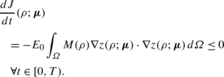 (76)
(76) -
If the functions ψ B (ρ) and ψ E (ρ) satisfy the hypothesis made in [92] for the bulk energy of the Cahn–Hilliard equation, the unique solution ρ converges to a steady state which minimizes the penalized objective functional J(ρ;μ) of the multiphase approach with respect to the initial solution ρ 0; in this manner, the optimization problem is converted to a time dependent one and its optimal solution ρ ∗ is obtained as ρ for t→∞.
-
The topology optimization problem is completely defined in the formulation by choosing the data h, f, ℂ0 and Ω, the function g(ρ) in Eq. (13), the mobility M(ρ), the initial condition ρ 0 (which also introduces the area/volume constraint V) and the parameters \(\boldsymbol{\mu}\in\mathcal{D}\).

In the current work we do not provide a rigorous analysis of the generalized Cahn–Hilliard equation for topology optimization problems. At this point, we only speculate on the possibility that the bulk ψ B (ρ) and especially the strain energy ψ E (ρ) functions could satisfy the hypothesis made in [92] for the existence and uniqueness of the solution ρ and its convergence to a steady state, the minimizer of J(ρ;μ); further limitations on the material interpolation model could be eventually deduced to fit such hypothesis. However, we observe that numerical tests exhibit the convergence of the solution to a steady state for any given initial solution, for which we feel that the validity of the considered phase field model could be shown also from an analytical point of view.
Remark 4
As observed in Remark 1, the minimum value of the penalized objective functional J(ρ;μ) does not coincides in general with the minimum value of the compliance J E (ρ) (19). For this reason, at the steady state of the phase transition, only a (local) minimum of J(ρ;μ) is obtained, while the minimum value of J E (ρ) can be obtained at an intermediate time t∈[0,T).
4.2 The Coupled System
The generalized Cahn–Hilliard equation (75) (or Eq. (73) in strong form) is written in terms of the phase variable ρ. However, in order to solve the problem it is necessary to evaluate the displacement u(ρ) by solving the elasticity equation (17) for a given value of ρ. In practice, for each t∈[0,T), there is a corresponding displacement \(\mathbf{u} \in\mathcal{V}\). For this reason, it is convenient to consider the phase ρ and the displacement u as two independent variables and rewrite the generalized Cahn–Hilliard equation as a coupled system of equations.
By recalling Eqs. (73), (71) and (15), the strong form of the coupled system is:

for some \(\boldsymbol{\mu}\in\mathcal{D}\). Also, for each t∈[0,T), we define the residual \(\widetilde{R}_{\rho}(\rho,\mathbf{u};\boldsymbol{\mu})(\phi) \in\mathbb{R}\) from Eq. (74) by recalling the potential \(\widetilde{z}(\rho,\mathbf{u};\boldsymbol {\mu})\) (71):

similarly, from Eq. (16), for each t∈[0,T), we redefine \(\widetilde{R}_{\mathbf{u}}(\rho,\mathbf{u}; \boldsymbol{\mu })(\mathbf{v}) \in\mathbb{R}\) to highlight the explicit dependency on ρ and u as:

Then, the coupled system of generalized Cahn–Hilliard and elasticity equations in weak form, which we will indicate as TO(μ), reads:

for some \(\boldsymbol{\mu}\in\mathcal{D}\) and the associated energy \(\widetilde{J}(\rho,\mathbf{u};\boldsymbol{\mu})\) defined in Eq. (37). We observe that the displacement u depends on the time t∈[0,T) implicitly trough the variation of the phase ρ. Indeed, in the elasticity equation no time derivatives appear, meaning that the displacement adapts instantaneously to the variation of the phase.
The reformulation of the generalized Cahn–Hilliard equation (75) (or Eq. (73)) into the coupled system TO(μ) (80) provides an approach to analyze the problem in terms of existence and uniqueness. Indeed, we notice that the coupled system (80) shows many analogies with the Cahn–Hilliard equation with elastic misfit, also known as the Cahn–Larchè model [65], for which the phase transition is also driven by elastic interactions of the material [45, 78]. In [45] the existence of a solution of such a system is proved as well as its uniqueness for a specific choice of the elastic energy; in [46] the corresponding discretized problem is analyzed. However, we remark that the Cahn–Larché equations and the coupled system TO(μ) (80) corresponding to the generalized Cahn–Hilliard equations are derived from different concepts. Indeed, the first equations follow from thermodynamical considerations and balance laws for the species and the momentum with ρ and u as independent variables. Conversely, the generalized Cahn–Hilliard equation is developed by considering the displacement variable as dependent on the phase variable u(ρ) and only the balance of the species is taken into account; the coupled system TO(μ) only represents a reformulation of such an equation.
4.3 Dimensionless Form of the Coupled System
We now rewrite the coupled system (80) in dimensionless form. With this aim, we introduce the dimensionless space and time coordinates:
and the phase and displacement variables:
where L 0 and T 0 are representative length and time scales, while the superscript ⋆ indicates dimensionless variables. Also, if we use E 0 as the representative Young modulus, we obtain:
and

while defining the reference surface and body forces  and f
0, we have:
and f
0, we have:

finally, the dimensionless mobility is:
Let us define the following dimensionless parameters which we indicate with the vector D=(D 1,…,D 5) such that:

we observe that the parameter γ is dimensionless, while the parameter λ assumes the same dimension as \(L_{0}^{2}\). Moreover, we define the dimensionless potential:
for which \(\widetilde{z}^{\star}(\rho^{\star},\mathbf{u}^{\star};\mathbf{D}) = D_{2} \widetilde{z}(\rho,\mathbf{u};\boldsymbol{\mu})\) and the dimensionless energy function:
for which \({\widetilde{\psi}^{\star}(\rho^{\star},\mathbf{u}^{\star};\allowbreak\mathbf{D}) = \frac{D_{2}}{E_{0}} \widetilde{\psi}(\rho ,\mathbf{u};\boldsymbol{\mu})}\). With these, we define from Eq. (78) the dimensionless residual \(\widetilde{R}^{\star}_{\rho}(\rho^{\star},\mathbf{u}^{\star};\allowbreak \mathbf{D})(\phi^{\star}) \in\mathbb{R}\ \forall t \in[0,T)\):

for which \(\widetilde{R}^{\star}_{\rho}(\rho^{\star},\mathbf{u}^{\star};\mathbf{D})(\phi^{\star}) = \frac{L_{0}^{4-d}}{\lambda M_{0}} \widetilde{R}_{\rho}(\rho,\mathbf{u};\boldsymbol{\mu})(\phi)\); similarly, from Eq. (79) we define \(\widetilde{R}^{\star}_{\mathbf{u}}(\rho^{\star},\mathbf{u}^{\star};\mathbf{D}) (\mathbf{v}^{\star}) \in\mathbb{R}\ \forall t \in[0,T)\) as:

with  . It follows that the dimensionless topology optimization problem in the phase field approach reads:

with \(\rho_{0}^{\star}= \rho_{0}\) and T ⋆=T/T 0. The corresponding dimensionless penalized objective functional (energy) follows from Eq. (89) as:
with \(\widetilde{J}^{\star}(\rho^{\star},\mathbf{u}^{\star};\mathbf{D}) = \frac{1}{E_{0}} \frac{L_{0}^{2-d}}{\lambda} \widetilde{J}(\rho,\mathbf{u};\boldsymbol{\mu})\); the same scaling occurs for \(\widetilde{J}_{E}^{\star}(\rho^{\star},\mathbf{u}^{\star})\), \(J_{B}^{\star}(\rho^{\star})\) and \(J_{I}^{\star}(\rho^{\star})\).
We notice that the topology optimization problem (92) fully depends on the dimensionless parameters D and the initial solution \(\rho^{\star}_{0}\), for which the principle of dimensional similitude can be applied. Also, it is possible to reduce the parametric dependence by setting D 1=1 and hence choosing the representative time scale as \(T_{0} = \frac{L^{4}_{0}}{\lambda M_{0}}\); it follows that the problem TO⋆(D) (92) depends on D=(D 2,…,D 5).
We observe from Eq. (91) that the dimensionless parameters D 4 and D 5 of Eq. (87) only affect the linear elasticity equation. The dimensionless parameters D 2 and D 3 are responsible for changing the optimal solution of TO⋆(D) once the data are set; indeed they control the balance of the strain, bulk and interfaces energies in the penalized objective functional (93). From Eq. (89), we deduce that if D 3 is very large, then the phase field solution is dominated by the minimum compliance term of the penalized objective functional. Conversely, if D 3→0, specifically if due to γ→0, TO⋆(D) solves the standard Cahn–Hilliard equation for the phase problem with the displacement u ⋆ depending on the distribution of ρ ⋆ in Ω ⋆. Also, since from Eq. (87) D 3=γD 2 and D 2∼1/λ, with λ related to the control of the thickness of the interfaces, we have that D 2 and D 3≫1, when sharp interfaces are required.
Remark 5
For the sake of simplicity, we henceforth omit the superscript ⋆ to indicate dimensionless quantities.
5 Numerical Approximation
In this section we discuss the numerical approximation of the topology optimization problem TO(D) (92) by using a similar approach to the one used in [50, 51] for phase field problems. In particular, for the spatial approximation we consider Isogeometric Analysis [35, 58], while for the temporal approximation we use the generalized-α method [32] with time adaptivity.
5.1 The Spatial Approximation
We consider design domains Ω described by a NURBS (or B-spline basis) [85], for both the two and three-dimensional cases. The use of Isogeometric Analysis for the spatial approximation of the PDEs allows us to encapsulate directly the geometry representation in the analysis, by using the same basis functions used to represent the geometry [35, 58]. In this manner, no geometrical approximations are introduced in the analysis of the topology optimization problem TO(D) (92).
Isogeometric Analysis provides a way to easily achieve high-order continuity in the approximated solution without introducing extra degrees of freedom. In particular, for the TO(D) problem, the use of globally C 1(Ω)-continuous basis functions is necessary to approximate the functional space \(\mathcal{H}\) of the phase variable ρ. Specifically, we consider basis functions of degree p≥2 defined by open knot vectors with equally spaced internal knots repeated at most p−1 times; in this manner we ensure that the basis functions are globally C 1(Ω)-continuous. We consider the same basis functions for the phase ρ and the displacement u.
We introduce the finite dimensional spaces \(\mathcal{H}_{h} \subset \mathcal{H}\) and \(\mathcal{V}_{h} \subset\mathcal{V}\), with the above mentioned properties, of dimensions \({n_{h,\rho} := \text{dim} (\mathcal{H}_{h} )}\) and \({n_{h,\mathbf{u}} := \text{dim} (\mathcal{V}_{h} )}\). Due to the properties of the NURBS basis, the essential boundary condition \(\nabla\rho\cdot\hat{\mathbf{n}}=0\) is easily introduced in the space \(\mathcal{H}_{h}\) by imposing equality of two consecutive control values of ρ normal to the boundary. We illustrate strong imposition of the essential boundary condition in Fig. 2 for a one-dimensional B-spline basis of degree 2. This also holds for NURBS and for the multidimensional case. For each t∈[0,T), \(\rho _{h} \in\mathcal{H}_{h}\) and \(\mathbf{u}_{h} \in\mathcal{V}_{h}\) have the representations:

with N A (x) the NURBS basis and n bf the number of basis functions; the corresponding test functions are:

Then the discrete TO h (D) coupled problem for any t∈[0,T) is:

where the discrete initial condition ρ 0,h is obtained as the L 2(Ω) projection of ρ 0 in the space \(\mathcal{H}_{h}\). The total number of degrees of freedom of TO h (D) is n h :=n h,ρ +n h,u . Finally, we introduce from Eq. (94) the vectors of control variables:

and, from Eqs. (90) and (91), the discrete residuals:

where \(\hat{\mathbf{e}}_{i}\), with i=1,…,d, represent the orthonormal basis of the space ℝd; for the sake of simplicity, we neglected the explicit dependency of the discrete residuals on D in Eq. (98).

B-spline basis of degree 2 and knot vector \(\varXi=\{\{0\}_{i=1}^{3},\allowbreak 0.2,0.4,\allowbreak 0.6,0.8,\{1\}_{i=1}^{3}\}\); the two external pairs of basis functions are marked with squares and circles to indicate that the corresponding control variables need to be equal to impose the boundary condition \(\nabla\rho\cdot\hat{\mathbf{n}}=0\) on ∂Ω
5.2 The Time Approximation
The time approximation of the TO(D) problem (92) represents a challenge similar to that for the Cahn–Hilliard equation due to the fourth-order term and significant nonlinearities. We use the generalized-α method; see [32, 60] and also [8, 50]. Moreover, since the solution of the topology optimization problem is obtained as the steady state solution of the coupled system (92), i.e. for t→∞ (or T sufficiently large), we need an adaptive time scheme that reduces the time step size when necessary and increases it as the solution approaches the steady state. We employ the same procedure proposed in [50] for the Cahn–Hilliard equation, which is based on an accuracy criterion and reduces the computational costs of the simulation while maintaining an adequate level of accuracy.
Very recently, a new second-order accurate, provably unconditionally stable, time integration algorithm for phase field models has been developed in [49]. This would provide a viable alternative to the generalized-α method.
5.2.1 Time Step Scheme
Let us subdivide the time interval [0,T) by introducing the discrete time vector \(\{t_{n} \}_{n=0}^{n_{ts}}\), with Δt n :=t n+1−t n the width of the time interval at the step t n , for which the control variables (97) are \(\dot{\mathbf{P}}_{n} = \dot{\mathbf{P}}(t_{n})\), P n =P(t n ) and U n =U(t n ). Then, if we interpret the variables \(\dot{\mathbf{P}}_{n+1}\) and P n+1 as independent, the generalized-α method for the TO h (D) problem at time step t n+1 reads from Eq. (98):

with \(\dot{\mathbf{P}}_{n}\) and P n given; the parameters α m , α f and δ∈ℝ, chosen on the basis of stability and accuracy considerations, define a specific generalized-α method. As described in [57, 60] we select α m , α f and δ as follows:

where ρ ∞∈[0,1] is the spectral radius of the amplification matrix at Δt→∞. See [57, 60] for further details.
The nonlinear system (99) is solved for each time step t n+1, for n=0,…,n ts −1, by means of a two stage predictor-multicorrector algorithm, for which the control variables at the time step t n+1 are obtained iteratively, where \(\dot{\mathbf{P}}_{n+1,(i)}\), P n+1,(i) and U n+1,(i), for i=0,1,…,i max , are the iterates and where i=0 indicates the predictor. At the predictor stage the control variables are initialized as:

At the multicorrector stage the following iteration steps are repeated for i=1,…,i max :
-
1.
Update the control variables following the last two relations of Eq. (99):
 (102)
(102) -
2.
Assemble the residuals:
 (103)
(103) -
3.
If the following stopping criteria on the relative norms of the residuals:
$$ \frac{\|\mathbf{R}_{\rho,(i)}\|}{\|\mathbf{R}_{\rho ,(0)}\|} < \mathit{tol}_R \quad \text{and} \quad\frac{\|\mathbf{R}_{\mathbf{u},(i)}\|}{\|\mathbf{R}_{\mathbf{u},(0)}\|} < \mathit{tol}_R $$(104)are satisfied for a prescribed tolerance tol R , set the control variables at time step t n+1 as \(\dot{\mathbf{P}}_{n+1}=\dot{\mathbf{P}}_{n+1,(i-1)}\), P n+1=P n+1,(i−1) and U n+1=U n+1,(i−1) and exit the multicorrector stage; else proceed to step 4.
-
4.
Define the consistent tangent matrices from Eq. (98):
 (105)
(105)where, by using Eq. (99), we have:
 (106)
(106) -
5.
Solve the following linear system in the variables Δ P n+1,(i) and Δ U n+1,(i):
 (107)
(107) -
6.
Update the control variables:
 (108)
(108)and return to step 1.


5.2.2 Time Adaptivity
We consider an adaptive scheme similar to the one proposed in [50], which is based on the comparison of the solutions obtained with the generalized-α method and the backward Euler method [88]. The backward Euler method can be obtained by setting α m =α f =δ=1 in the generalized-α method.
The adaptive time scheme starts, for each time step t n+1, n=0,…,n ts −1, with the given control variables \(\dot{\mathbf{P}}_{n}\), P n and U n , and a given time step Δt n , typically that used at the previous time step. Then, in the adaptive algorithm the following steps are repeated for l=1,…,l max , starting with Δt n,(0)=Δt n−1 (or, if n=0, with Δt n,(0)=Δt 0):
-
1.
Compute the control variables \(\dot{\mathbf{P}}_{n+1,(l-1)}\), P n+1,(l−1) and U n+1,(l−1) with the generalized-α method of Sect. 5.2.1 for Δt n,(l−1).
-
2.
Compute the control variables \(\dot{\mathbf{P}}^{BE}_{n+1,(l-1)}\), \(\mathbf{P}^{BE}_{n+1,(l-1)}\) and \(\mathbf{U}^{BE}_{n+1,(l-1)}\) by means of the backward Euler method for Δt n,(l−1).
-
3.
If the generalized-α or the backward Euler methods are not converging (i.e. the predictor-multicorrector algorithm of Sect. 5.2.1 is not convergent), reduce the time step by means of a safety coefficient χ NC ∈(0,1), update Δt n,(l) as:
$$ \varDelta t_{n,(l)} = \chi_{NC} \varDelta t_{n,(l-1)}, $$(109)and return to step 1; else proceed to step 4.
-
4.
Evaluate the relative error associated to Δt n,(l−1):
 (110)
(110) -
5.
Update the time step size according to the following formula:
$$ \varDelta t_{n,(l)} = \chi_{n,(l-1)} \varDelta t_{n,(l-1)}, $$(111)where:
$$ \chi_{n,(l-1)} := \min\biggl\{ \chi_A \biggl( \frac{\mathit{tol}_A}{e_{n+1,(l-1)}} \biggr)^{1 / 2}, 1+\chi_{GR} \biggr \}, $$(112)with tol A a prescribed tolerance, χ A ∈(0,1) a suitable safety coefficient and χ GR >0 the maximum growth rate admitted.
-
6.
If e n+1,(l−1)≥tol A , return to step 1. Otherwise, update the control variables \(\dot{\mathbf{P}}_{n+1}= \dot {\mathbf{P}}_{n+1,(l-1)}\), P n+1=P n+1,(l−1), U n+1=U n+1,(l−1) and the time step Δt n =Δt n,(l), and exit the loop.

We observe that on the basis of the previous algorithm, one of following three situations occurs after step 6:
-
if \(e_{n+1,(l-1)} < \chi_{A}^{2} \mathit{tol}_{A}\), the time step size is increased, the control variables of step 1 are considered valid and the loop ends;
-
if \(\chi_{A}^{2} \mathit{tol}_{A} \leq e_{n+1,(l-1)} < \mathit {tol}_{A}\), the time step size is reduced, the control variables of step 1 are still considered valid and loop terminates;
-
if e n+1,(l−1)≥tol A , the time step size is reduced, the control variables of step 1 are invalid and the steps 1–6 are repeated.
Since the steps 1 and 2 are computationally expensive, the occurrence of the last case should be minimum; as pointed out in [50], this is the case if good choices for the parameters tol A and χ A are made.
6 Selection of Parameters and Optimal Design
In Sect. 4.3 we provided the dimensionless form of the topology optimization problem (92), which we proposed to solve numerically by means of Isogeometric Analysis and the generalized-α method in Sect. 5. However, as already pointed out, the solution of the TO(D) problem depends on the dimensionless parameters D, which depend on parameters \(\boldsymbol{\mu}\in\mathcal{D}\) introduced in Sect. 2.3. In this section we address the issue of the choice of the parameters \(\boldsymbol{\mu}\in\mathcal{D}\) and the mesh dependency effect, we select the interpolation function g(ρ) (25) and the bulk energy ψ B (ρ) (33), we describe the continuation method which could be used for topology optimization in the phase field approach, and we discuss the choice of the initial solution ρ 0. Finally, we discuss the strategy for the identification and selection of the optimal topological design.
6.1 The Choice of the Parameters \(\boldsymbol{\mu}\in \mathcal{D}\) and Mesh Dependency
The dimensionless parameters D (87) depend both on the data of the problem and the parameters \(\boldsymbol{\mu }=(\lambda,\gamma) \in\mathcal{D}\); in particular, only the dimensionless parameters D 2 and D 3 and the representative time scale T 0 are related to \(\boldsymbol{\mu}\in\mathcal{D}\), since we set D 1=1.
For the choice of the parameter λ we adopt similar considerations to the ones made in [50, 51]. The Cahn–Hilliard equation converges for λ→0 (see Eq. (45)) to a thermodynamically consistent sharp-interface model, for which the representative length scale of the interface is related to \(\sqrt{\lambda}\). Similarly, for the generalized Cahn–Hilliard equation for topology optimization, the value of λ should be sufficiently small in order to provide realistic results with sharp interfaces between the material and the void. Moreover, λ is responsible for the number of holes appearing in the optimal topology, since in general it is associated with the interface energy ψ I (ρ) of Eq. (29).
From a numerical point of view, we observe that the computational mesh used for the spatial approximation should be fine enough to capture the thin layers between the material and void. For these reasons, following from the dimensional considerations of Sect. 4.3, we assume that the thickness of the interfaces depends on the computational mesh and the parameter λ is chosen as [50]:
where h is the characteristic length of the computational mesh, defined as:
with V i the area/volume of the i-th element of the mesh composed by n el elements. The parameter \(\overline{\lambda}\) is dimensionless and it is chosen by the user. Indeed, it is difficult to specify at this point what value \(\overline{\lambda}\) should assume since it depends in general on the data of the topology optimization problem; for example, in [50] it is shown that for the Cahn–Hilliard equation \(\overline{\lambda}\) should depend on the area/volume V covered by the material in Ω. According to this choice, the thickness of the interfaces is roughly equal to \({\sqrt{\lambda}} = {\sqrt{\overline{\lambda}} h}\), with shaper interfaces for finer meshes, which in turn allow more detailed topologies to be obtained. On the other hand, the parameter λ introduces a mesh dependency in the topology optimization problem through D 2, D 3 and T 0; this represents an undesired issue in topology optimization since the optimal distribution of the material in the design domain Ω changes with the spatial approximation used. Moreover, in general, the convexity of the discrete objective functional is altered and different, and more local minima may appear by refining the mesh. However, for “sufficiently” fine meshes with respect to a fixed thickness of the interfaces \({\sqrt{\lambda}}\), the improved resolution does not alter the convexity structure of the problem, but only allows for a more accurate representation of the interfaces. For this reason, we believe that in the phase field and multiphase approaches, the mesh dependency of the optimal topology could be reduced and eventually eliminated by using a fixed value of h, say h 0, for the evaluation of the parameter λ for all the computational meshes having h≤h 0.
The choice of the parameter γ is important. A value of γ that is too small will cause the objective functional to be dominated by the interface and bulk energy terms (i.e. by the relaxation of the total variation of the material density function approximating the perimeter of the interfaces); if γ is too large, divergence may occur. The role of γ is to properly balance the strain energy function ψ E (ρ) with respect to the bulk and interface energy functions, ψ B (ρ) and ψ I (ρ), in Eq. (33). However, it is difficult to determine a priori a suitable value for γ by means of dimensional analysis; this is due to the fact that the strain energy strongly depends on data of the topology optimization problem, which are not represented by the dimensionless parameters, such as the shape of the design domain Ω and the direction of the body and surface forces f and h. In [119, 120], the values differ from one test case to another; in [24, 107] the choice of γ appears to be arbitrary, while in [21] it is made by trial and error. In order to ensure a proper balance of the strain energy with respect to the other energies in (37), we propose to decompose the dimensionless parameter γ as:
where \(\overline{\gamma}\) is a positive parameter chosen by the user and γ E is computed from Eqs. (87) and (89) as:
with ρ 0 the initial density, \(\psi_{E}(\rho_{0}) = \widetilde{\psi}_{E}(\rho_{0},\mathbf{u}(\rho_{0}))\) from Eq. (84) and, in order to make γ E independent of \(\overline{\lambda}\), from Eqs. (87) and (113) we set
Finally, from Eqs. (113) and (116), we obtain from Eq. (87) that the dimensionless parameters D 2 and D 3 are:
while \({T_{0} =\frac{L_{0}^{4}}{\overline{\lambda}h^{2} M_{0}}}\), since we have set D 1=1.
At this point, the topology optimization problem TO(D) still depends on the arbitrary choices made for the parameters \(\overline{\lambda}\) and \(\overline{\gamma}\). However, numerical tests reveal that these dimensionless parameters vary in a limited range of values for different topology optimization problems; indeed, we typically select \(\overline{\lambda}\in[0.5,6.0]\) and \(\overline{\gamma}\in[0.5,4.0]\). On the other hand, these parameters allow the user to modify the outcome of the topology optimization results. In particular, the number of holes of the optimal topology can be increased or decreased by decreasing or increasing \(\overline{\lambda}\), respectively.
6.2 The Choice of the Interpolation Function g(ρ) and the Bulk Energy Function ψ B (ρ)
As anticipated in Sect. 2.2 the interpolation function g(ρ) is typically chosen as g(ρ)=ρ P (see Eq. (25)), with P≥3 for an isotropic material with ν 0=1/3. We consider a similar interpolation rule which ensures that ρ exceeds a minimum value ρ min and, to avoid numerical issues, the condition that the first and second derivatives of such interpolation function are zero at the pure phases 0 and 1. In particular, we consider:
with f(ρ) the following C 2-continuous function:
and b(ρ) a C 2-continuous third-degree B-spline in ρ obtained with the open knot vector \(\mathcal{S}=\{\{\rho_{1}\}_{i=1}^{4}, \rho_{2},\ldots,\rho_{5},\allowbreak \{\rho_{6}\} _{i=1}^{4}\}\) and the control points \(\mathcal{P}=\{0,0,0,0,1,1,1,1\}\); see [85]. In Fig. 3 we compare the function f(ρ) with the typical SIMP function, f SIMP (ρ), which is only C 0-continuous in [0,1], where:
also, we compare the interpolation function g(ρ) (119) with the SIMP function say g SIMP (ρ)=f SIMP (ρ)P for P=3; in particular, we choose ρ min =0.1 and \(\mathcal{S} =\{\{0.055\}_{i=1}^{4},0.065,0.075,0.925,0.935,\{0.945\} _{i=1}^{4}\}\).

Functions f(ρ) (—) and f SIMP (ρ) (- -) (top) and interpolation functions g(ρ) (—) and g SIMP (ρ) (- -) (bottom)
We remark that the choice of the interpolation function g(ρ) plays a crucial role in the formulation of the topology optimization problem in the multiphase and phase field approaches. Indeed, the qualitative features of the optimal design strongly depend on the variation of the elastic properties through the interfaces between the material and void. For this reason, alternative and eventually more effective choices of g(ρ) should be investigated.
For the bulk energy function ψ B (ρ) we select the following C ∞-continuous function in ρ:
with β 1, \(\beta_{2} \in\mathbb{R}^{+}_{0}\). This choice allows naturally steep bounds on the pure phases 0 and 1 but avoids any singularities. In Fig. 4 we plot ψ B (ρ) for ρ in [0,1] corresponding to the values β 1=0.5 and β 2=50, which we will select for the numerical tests.

Bulk energy function ψ B (ρ)
6.3 The Continuation Method
In Remark 2 we introduced the parameter κ in view of the use of the continuation method to solve topology optimization problems in the multiphase approach as done for example in [21, 24]. This procedure can be extended to the case of the topology optimization problem in the phase field approach by following the formulation outlined in Sect. 4 with the penalized objective functional J κ (ρ;μ k ) (42). The dimensionless parameters D 1, D 2 and D 3 of Eq. (87) are modified as:
for which D κ :=(D κ,1,D κ,2,D κ,3,D 4,D 5) and \(D_{3}^{\kappa}\) can be chosen as:
for some γ κ , similar to Eq. (118). The characteristic time is \({T_{\kappa,0}:=\frac{1}{\kappa}T_{0}}\), corresponding to the choice D κ,1=1, while the penalized objective functional scales with the quantity \({\frac{1}{E}_{0} \frac {L_{0}^{2-d}}{\kappa\lambda}}\).
We propose the following procedure for the continuation method:
-
1.
set the data for the topology optimization problem;
-
2.
choose an initial solution ρ 0 such that ∫ Ω ρ 0 dΩ=V;
-
3.
select the parameters \(\overline{\lambda}\) and \(\overline{\gamma}\) of Eqs. (113) and (115), respectively;
-
4.
choose the computational mesh for the spatial approximation and compute h as in Eq. (118);
-
5.
compute the parameter λ from Eq. (113) and the dimensionless parameter D 2 from Eq. (87);
-
6.
select a discrete set \(\mathbb{K}\) of values for the parameter κ, where \(\mathbb{K} := \{\kappa_{m} \}_{m=1}^{M}\), with κ 1>⋯>κ M >0 and M the number of continuation levels;
-
7.
repeat the following operations for the m=1,…,M continuation levels:
-
1.
if m=1 set ρ 0,h,(1)=ρ 0,h , otherwise, for m≥2, set ρ 0,h,(m)=ρ h,(m−1) for t=T, where ρ h,(m−1) is the steady state solution obtained at the continuation level m−1;
-
2.
set κ=κ m and compute the dimensionless parameters D κ,(m) from Eqs. (87), (123) and (124) for \(\gamma_{\kappa}= \overline{\gamma}\, \gamma_{E,\kappa}\), where γ E,κ is computed from Eq. (116) by replacing ρ 0 with ρ 0,h,(m);Footnote 5 also compute T κ,0,(m);
-
3.
solve the TO h (D κ,(m)) problem (96) by using Isogeometric Analysis and the generalized-α method with the adaptive scheme outlined in Sect. 5 to obtain the steady state solution ρ h,(m) for t=T.
-
1.
The choice of the set \(\mathbb{K}\) is arbitrary as well as are the choices of the parameters \(\overline{\lambda}\) and \(\overline{\gamma}\). As a general indication, if the number of continuation levels M is too large, high computational cost is associated with the solution of the topology optimization problem with this approach. On the other hand, if M is too small or the ratios κ m−1/κ m ≫1, then convergence may not occur.
The use of the continuation method allows, for a proper selection of the set \(\mathbb{K}\), to use smaller values for \(\overline{\lambda}\) than typically used when the TO h (D) problem (96) is solved as a single simulation; this is due to the property of the continuation method to approach the optimal solution as a sequence of intermediate optimal results.
6.4 The Choice of the Initial Solution ρ 0
In the phase field approach the topology optimization problem allows one to obtain the optimal solution as the steady state of the phase field model which minimizes a penalized objective functional starting from an initial solution ρ 0. In the previous sections we only required that ρ 0 satisfy the area/volume constraint, ∫ Ω ρ 0 dΩ=V. It follows that, even with this constraint satisfied, the choice of ρ 0 is arbitrary.
Different strategies for the choice of ρ 0 have been considered in the literature, since the initial distribution of the material could largely influence the optimal topology in the minimum compliance case depending on the approach used. In general, the more ρ 0 is similar to the optimal solution, the more rapid will be the convergence of the topology optimization method; however, this situation prefigures an a priori knowledge of the optimal solution. For the SIMP approach [13] the initial solution is chosen as ρ 0=ρ V , with ρ V :=V/|Ω|, even if ρ 0 often is allowed to violate the area/volume constraint, which is later restored during the optimization procedure. In the level set approach [4, 37] ρ 0 is chosen as a 0–1 distribution of material with holes such that the area/volume constraints is satisfied; the initial number of holes affects the number of holes in the optimal topology and plays a crucial role in the definition of the final topology. However, it is shown in [117] by means of numerical examples that when the capability of hole nucleation is introduced in the level set method, the dependence of the optimal solution on the initial one is reduced. Initial solutions in the 0–1 configurations are also chosen in [107] for topology optimization problems formulated with the Cahn–Allen equation, which shows a strong dependence of the optimal solution on the initial one. For the phase field approach of [119, 120] using the generalized Cahn–Hilliard equation, ρ 0 is a random distribution around the average value ρ V .
In this work, we typically choose ρ 0=ρ V . However, the continuation method of Sect. 6.2 can be effectively used to provide a suitable initial solution ρ 0 without any a priori knowledge of the optimal solution.
6.5 The Identification of the Optimal Design
By recalling Remarks 1 and 4, we observe that the steady state solution does not necessarily provide the minimum value of the compliance J E (ρ) (19) which we aim at minimizing, but rather a minimum of the penalized objective functional J(ρ;μ) (32). However, in the phase field approach of Sect. 4.1, one can eventually identify a time, say \(t^{*}_{E}< T\), for which the minimum value of J E (ρ) is reached by tracking and observing the behavior of the compliance J E (ρ) during the phase transition; i.e. we define:
with the associated material distribution \(\rho_{E}^{*} := \rho(t_{E}^{*})\) and the minimum value of the compliance:
As for the penalized functional J(ρ;μ), we notice that the minimum compliance depends on the choice of the parameters \(\boldsymbol{\mu}\in\mathcal{D}\), for which \(\rho_{E}^{*} = \rho_{E}^{*}(\boldsymbol{\mu})\) and \(t^{*}_{E} = t^{*}_{E}(\boldsymbol{\mu})\). Provided that at \(t=t^{*}_{E}\) the phases are fully separated, one can identify the distribution of the material density function \(\rho^{*}_{E}\) as the optimal topological design for some \(\boldsymbol{\mu}\in \mathcal{D}\) rather than ρ ∗ as in Eq. (41) and Sect. 4.1.Footnote 6 We remark that, due to the non-monotone behavior of the compliance energy J E (ρ) in time, it is necessary to let the phase transition evolve to the steady state to prevent the selection of a local minimum of J E (ρ). Also, we observe that, when the continuation method of Sect. 6.3 is used, the minimum compliance \(J^{*}_{E}\) is often obtained at the steady state of the last continuation level.
Finally, the geometric information on the optimal topology is obtained by means of the contour lines corresponding to \(\rho^{*}_{E} = 0.5\), or depending on the case, ρ ∗=0.5, provided that the separation of the phases in the pure ones has already occurred.
7 Numerical Tests
In this section we solve and discuss numerical problems in two and three-dimensions; we also highlight the features of the proposed method by means of two-dimensional tests. The numerical values considered for the numerical simulations and the implementation aspects are also reported.
7.1 Numerical Values and Implementation Aspects
For all the simulations reported the following numerical values are considered:
-
for the tensor ℂ0 (see Eq. (13)), we choose E 0=200⋅109 J/m and ν 0=1/3 for the plane strain two-dimensional problems and the three-dimensional problems;
-
for the representative quantities of Sect. 4.3, we choose L 0=1 m, T 0 such that D 1=1, M 0=1 m2/s,
 (for which D
4=1000) and f
0=0 N/m3 (no body force is considered for which D
5=0);
(for which D
4=1000) and f
0=0 N/m3 (no body force is considered for which D
5=0); -
the interpolation g(ρ) and the bulk energy ψ B (ρ) functions are chosen as in Sect. 6.2 with P=3 and the mobility is assumed constant, M(ρ)=M 0.
 (for which D
4=1000) and f
0=0 N/m3 (no body force is considered for which D
5=0);
(for which D
4=1000) and f
0=0 N/m3 (no body force is considered for which D
5=0);For the numerical approximation we consider:
-
for the Isogeometric spatial approximation of Sect. 5.1, we choose a NURBS (or B-splines) basis of degree p=2 and numerical integration is performed using 3×3 Gauss quadrature (3×3×3 in three-dimensional problems); this represents a very conservative approach. The study of more efficient quadrature schemes for NURBS was initiated in [59]; further investigations are ongoing;
-
for the time step scheme of Sect. 5.2.1 we choose ρ ∞=1/2 (for which α m =5/6, α f =2/3 and δ=2/3 from Eq. (100)), with the tolerance for the stopping criterion (104) tol R =10−4 and the maximum number of steps set equal to i max =7;
-
for the time adaptivity of Sect. 5.2.2 we select the initial time step Δt 0=10−12 and the final time T=102, χ NC =0.5 in Eq. (109) to reduce the time step in case of divergence of the generalized-α or backward Euler methods, and χ A =0.85, χ GR =0.2 and tol A =10−3 in Eq. (112) for the time update and stopping criterion;
-
the numerical solution of the spatial approximation is obtained by using the Bézier extraction methods presented in [18] (Bézier extraction provides a localized representation of the globally smooth basis that can be implemented in shape function routines in existing finite element codes);
-
the problem is solved using a parallel C++ code based on Trilinos [56] and MPI;
-
the linear system (107) is solved with the “monolithic” approach by means of the GMRES method preconditioned by an Algebraic Multigrid strategy with Smoothed Aggregation [47]; the dimension of the Krilov space is set equal to 700–1,000 and the stopping criterion is based on the relative residual with tolerance equal to 10−6.Footnote 7
Remark 6
The solution of the linear system (107) is particularly challenging for fine meshes, especially for three-dimensional problems; this is due to the nature of the block matrices involved in the global matrix. Indeed, the matrix K ρρ,(i) radically changes behavior as time evolves: when Δt is small, far from the steady state, the mass matrix dominates over the fourth-order stiffness matrix in K ρρ,(i) and convergence occurs in a relatively small number of GMRES steps. On the contrary, when Δt is large, many more steps are required. The block matrix K uu,(i) represents the stiffness matrix of the linear elastic problem, with elastic properties depending on the distribution of the phase variable ρ; see Eqs. (13) and (119). The properties of such a matrix abruptly change when passing through the interfaces and GMRES could suffer divergence issues when sharp interfaces are generated, especially in the parallel setting. If necessary, a way to partially overcome this inconvenience consists of enforcing the development of the interfaces over a sufficiently high number of mesh elements by suitably tuning the parameter \(\overline{\lambda}\) (113). Additionally, the off-diagonal block matrices K ρ u,(i) and K u ρ,(i) could further degrade the conditioning properties by rendering the full matrix “less symmetric.” We believe that an ad hoc preconditioner should be developed to take into account all these features while solving the linear system in the “monolithic” approach; we notice that this could be required even if the system (107) is eventually solved with a “staggered” approach. This was not pursued in the present work.
On the basis of the parameters above mentioned, a typical two-dimensional simulation with a mesh with 320×160 elements converges in about n ts =1,000–1,200 time steps; time adaptivity converges in one iteration with few exceptions for a limited number of time steps (typically only 1–10). In each time step the generalized-α method typically converges in one to four Newton iterations (likewise for the backward Euler method) and no, or a few, restarts with forced reduction of the time step are required due to divergence. For the same simulation, the solution of the linear system (107) requires a number of GMRES iterations comprised between 7 and 500 depending on the time step Δt and time t. In general, the smaller is the thickness of the interface for a given mesh (related to the parameter \(\overline{\lambda}\) of Eq. (113)) and/or the larger the parameter \(\overline{\gamma}\) of Eq. (115), the slower is the convergence of the simulation to the steady state solution; indeed, in these cases, we could incur a large number of time steps and time step adaptions, and a large number of Newton iterations in the generalized-α and backward Euler methods and, consequently, slow convergence of the GMRES linear solver.
7.2 Two-Dimensional Problems
We discuss two-dimensional topology optimization problems in order to highlight the features and properties of the method. We consider design domains represented by B-splines and NURBS bases.
7.2.1 Test 1
The topology optimization problem for Test 1 is represented in Fig. 5. We consider a rectangular design domain Ω with zero displacement boundary conditions on the left edge and the vertical traction  acting on the d
2-part of the right edge. We assume L=2.00 m, H=1.00 m, d
1=0.45 m and d
2=0.10 m. The fraction of the volume of Ω to be covered by the material is V/|Ω|=0.35. The design domain Ω is represented with a B-spline basis with the control points such that there is a linear mapping between the parametric domain and Ω.
acting on the d
2-part of the right edge. We assume L=2.00 m, H=1.00 m, d
1=0.45 m and d
2=0.10 m. The fraction of the volume of Ω to be covered by the material is V/|Ω|=0.35. The design domain Ω is represented with a B-spline basis with the control points such that there is a linear mapping between the parametric domain and Ω.

Test 1. Design domain Ω, surface force h and displacement constraints
For the numerical solution of the problem we consider a mesh with 320×160 elements, for which the dimensionless mesh size is h=0.00625. Also, we select the parameters \(\overline{\lambda}=6.0\) and \(\overline{\gamma}= 1.0\) for the definition of the dimensionless parameters D 2 and D 3 (see Eqs. (113), (115) and (118)); the parameter γ E =1.247⋅104 is selected from Eq. (116). The dimensionless parameters are D 2=4.267⋅103 and D 3=5.322⋅107, with the characteristic time T 0=4.267⋅103. We indicate this problem as Test 1.1. In Fig. 6 we present the evolution of the phase (material density) variable ρ by showing it at significant time steps; the initial solution is set as ρ 0=ρ V =V/|Ω|. The color scale is from blue to red for values of ρ from 0 to 1. As we can deduce from Fig. 7(top), the distribution of the material is driven at the initial steps by the above-average values of the strain energy function ψ E ; in this case, the material is distributed around the Γ D boundary and where the load h is applied. The phase separation occurring in these areas of the design domain is due to the generalized Cahn–Hilliard model which is mass/volume conservative. At these stages we can observe distributions of the material density function which are reminiscent of Michell type structures, see e.g. [13, 70]. As time evolves, the separation of the phases is mostly completed and the structure tends to simplify; this is due to the fact that the bulk, interface and strain energies (i.e., J B , J I and J E , respectively) are all contributing to the minimization of the objective functional J (see Eqs. (34) and (39)). The steady state represents the optimal topology in terms of the objective functional J, which reaches its minimum with respect to the initial value (for ρ=ρ 0 at t=0); it is also possible to see from Fig. 7(bottom) that the average value of the strain energy function ψ E is also much lower at the steady state. However, the optimal topology at the steady state does not necessarily represent the stiffest structure with the specified data as pointed out in Sect. 6.5; indeed, as is occurring in this case, the minimum value of J E (\(J^{*}_{E}\)) is obtained at an intermediate step \(t^{*}_{E}<T\) and before the steady state is reached. This fact is highlighted in Fig. 8 where the behavior of the objective functional J and the energies J E , J B and J I is plotted vs. the dimensionless time t. The objective functional J is monotonically decreasing in time as expected since it is a Liapunov functional (see Eq. (76)), even if this property does not hold for the energies J E , J B and J I . The large drop of J B is due to the phase separation and the evolution of J I to the creation of the interfaces and the following simplification of the topology during the evolution in time. The strain energy J E is also subject to a large and desired drop, even if its minimum value is reached at an intermediate step and not at the steady state. The fact that the steady state solution does not represent a fully optimal design can also be deduced from Fig. 7(bottom) where the distribution of the strain energy function ψ E highlights areas of the material which do not fully participate in carrying the load. We obtain that the initial value of the objective functional J decreases by 79.29 % at the steady state, while J E decreases by 86.33 %; the minimum value of J E (\(J^{*}_{E}\)) representing the real goal of the topology optimization is obtained at \(t=t^{*}_{E}=6.528 \cdot10^{-4}\) with a drop of 87.84 %; this represents a significantly smaller value by 11.05 % with respect to the one reached at the steady state. The topologies of these configurations are radically different; consequently, we can select the configuration for which J E is minimum as the optimal topology from a design point of view. The geometrical information is extracted from the solution by the contour lines corresponding to the value ρ=0.5. In Fig. 9 we show the evolution of the time step Δt n vs. time t, which is chosen adaptively according to the scheme presented in Sect. 5.2.2. We observe the large change in the value of Δt n from 10−12 to 18.8 occurring in a relatively small number of

Test 1.1. Evolution of the phase (material density) variable ρ in time for mesh size 320×160 with \(\overline{\lambda}=6.0\) and \(\overline{\gamma}= 1.0\)

Test 1.1. Distribution of the strain energy function ψ E (dimensionless) in the design domain Ω (initial and at the steady state); logarithm scale

Test 1.1. Normalized energies J (black), J E (red), J B (blue) and J I (green) vs. time t (top) and detail (bottom); the minimum value of J E (\(J^{*}_{E}\)) is indicated by an × (Color figure online)

Test 1.1. Time step Δt vs. time t (dimensionless) as selected by the adaptive time scheme (top) and detail (bottom)
time steps, 1,198 in this case; also, we observe how the intermittent nature of the phase field model is apparent in the drop of the value of Δt n required at some times steps. As a final consideration regarding the numerical scheme, we observe that the mass/volume constraint is adequately satisfied during the evolution in time, since the relative error with respect to the initial value of the volume fraction is practically negligible and below the 4.90⋅10−6 % threshold for all the time steps.
Finally, we discuss the results of the topology optimization for different values of the parameters \(\overline{\lambda}\) and \(\overline{\gamma}\) with respect to the ones previously selected; this test is referred to as Test 1.2. The goal is to show that a large value of \(\overline{\lambda}\) leads to optimal topologies with large interfaces and eventually to reduced minimizations of the strain energy J E . Similarly, if the value of \(\overline{\gamma}\) is too small, the phase transition leads to solutions principally driven by the Cahn–Hilliard terms, the reduction of J E would be limited in this case and the topology would have few or no holes. Ideally, as discussed in Sect. 6.1, one would select the smallest possible value of \(\overline{\lambda}\) and the largest of \(\overline{\gamma}\) which would lead to the steady state without the occurrence of divergence issues.Footnote 8 In Fig. 10(left) we present the topologies corresponding to the minimum value of J E (top) and to the steady state (bottom) for the parameters \(\overline{\lambda}= 12.0\) (twice that for Test 1.1) and \(\overline{\gamma}= 1.0\); the contour lines for ρ=0.5 of the solutions of Test 1.1 are highlighted. We can observe larger interfaces with respect to the previous case (about \(\sqrt{2}\) larger) and, even if the configuration at the steady state is very similar to the one of Test 1.1, the decrease in the values of J and J E is significantly different. Indeed, the drops of J and J E at the steady state are 74.71 % and 85.27 %, respectively (for Test 1.1 they were 79.29 % and 86.33 %); at its minimum (\(J^{*}_{E}\)), the drop of the strain energy J E is 86.61 %, a value larger by 10.12 % with respect to the one obtained in Test 1.1. Even more significant differences can be obtained for larger values of the parameter \(\overline{\lambda}\). In Fig. 10(right) we highlight the topologies obtained with the parameters \(\overline{\lambda}=6.0\) and \(\overline{\gamma}=0.2\) (1/5 of Test 1.1); the configurations corresponding to the minimum value of J E and at the steady state are presented together with the contour lines for ρ=0.5 corresponding to Test 1.1. The thickness of the interfaces between the phases is the same as in Test 1.1, even if the topologies exhibit significant changes. Also, the relatively “small” value of \(\overline{\gamma}\) leads to a nonsymmetric solution at the steady state since the symmetric configuration is unstable from the point of view of the phase field problem (a bifurcation from a symmetric configuration occurs during the phase transition). The decrease of J and J E at the steady state are 79.62 % and 80.21 %, respectively, with the value of J E being 34.35 % larger than in Test 1.1; similarly, the drop of J E at its minimum is 83.05 %, 39.39 % larger than in Test 1.1. Notice that in the limit case \(\overline{\gamma}=0.0\), the solution coincides with the Cahn–Hilliard one, which in this case exhibits a topology with a vertical rectangle.

Test 1.2. Phase (material density) variable ρ for mesh size 320×160 with \(\overline{\lambda}=12.0\) and \(\overline{\gamma}= 1.0\) (left) and \(\overline{\lambda}=6.0\) and \(\overline{\gamma}= 0.2\) (right); solutions for minimum value of J E (\(J^{*}_{E}\)) (top) and at the steady state (bottom). The contour lines represent the topologies obtained in Test 1.1 for \(\overline{\lambda}=6.0\) and \(\overline{\gamma}= 1.0\)
7.2.2 Test 2
For Test 2, we consider a quarter ring with inner radius R IN =1.00 m and outer radius R OUT =2.00 m as shown in Fig. 11. The surface force h is applied at the top-left tip of the design domain Ω along a boundary segment of length s=π/10 m; no displacement boundary conditions are applied at the bottom of Ω. The volume fraction of Ω to be occupied by the material is set equal to V/|Ω|=0.35. We represent the design domain Ω by means of a NURBS basis of degree 2 [85] for which, by using Isogeometric Analysis, the exact representation of the geometry is maintained through the analysis and the topology optimization procedure.

Test 2. Design domain Ω, surface force h and displacement constraints
We solve the topology optimization problem with a mesh composed by 320×160 elements with the larger number along the circumferential direction; the dimensionless mesh dimension is h=9.818⋅10−3. We select the parameters \(\overline{\lambda}= 5.0\) and \(\overline{\gamma}= 1.5\), for which we have D 2=2.075⋅103 and D 3=2.275⋅107 with the computed γ E =7.309⋅103. We indicate this test as Test 2.1. In Fig. 12 we present the evolution in time of the material density starting from the initial solution ρ 0=ρ V =V/|Ω| toward the steady state; intermediate significant solutions are presented, including the one corresponding to the minimum value of J E (\(J^{*}_{E}\)). We observe that, even if such solution does not exhibit a complete phase separation, useful topological information can still be obtained and the configuration can be used for further design investigation. In Fig. 13 we highlight the behavior of the objective functional J and the energies J E , J B and J I vs. the time; a detailed view around the minimum value of J E is also presented. The decrease of the value of J is 75.56 % at the steady state, while for J E it is 84.35 %; at its minimum, which occurs at \(t=t^{*}_{E}=5.420 \cdot10^{-5}\) (dimensionless), the decrease of J E is 86.25 %, 12.12 % smaller than at the steady state.

Test 2.1. Evolution of the phase (material density) variable ρ in time for mesh size 320×160 with \(\overline{\lambda}=5.0\) and \(\overline{\gamma}= 1.5\)

Test 2.1. Normalized energies J (black), J E (red), J B (blue) and J I (green) vs. time t (top) and detail (bottom); the minimum value of J E (\(J^{*}_{E}\)) is indicated by an × (Color figure online)
We now discuss the mesh dependency effect in Test 2.2. With this aim, we solve the same problem discussed previously with different mesh sizes and values of the parameter λ affecting the dimensionless parameters D 2 and D 3 (see Eq. (87)). If the goal of the topology optimization is to obtain sharp interfaces and detailed optimal topologies, fine meshes need to be used since, from Eq. (113), the parameter λ is selected as \(\lambda= \overline{\lambda}h^{2}\), with h indicative of the mesh size. However, as already mentioned in Sect. 6.1, this introduces a mesh dependency effect on the solution, since the dimensionless parameters D 2 and D 3 vary with the mesh. On the other hand, we believe that the mesh dependency issue can be quickly reduced or eliminated in the phase field approach by using a fixed value of h=h 0 for all the meshes having h≤h 0. In Fig. 14(right) we show the optimal topologies obtained at the steady states for different mesh sizes (80×40, 160×80 and 320×160) for \(\overline{\lambda}= 5.0\) and \(\overline{\gamma}=1.5\); once h 0 is set to be the representative dimensionless size of the mesh 80×40 (h 0=0.03927), we select h=h 0,h 0/2,h 0/4 for the three meshes, respectively. In this case, we observe that, not only does the thickness of the interfaces change from one mesh to the other, but also the optimal topologies significantly vary. Conversely, if we assume a constant value of h=h 0 for all the meshes, the thickness of the interfaces between the phases and the optimal topologies remain the same; see Fig. 14(left) where we considered \(\overline{\lambda}= 1.0\) and \(\overline{\gamma}=2.0\) to show shaper interfaces (the same result of Fig. 14(top-right) would have been obtained for all three meshes with \(\overline{\lambda}= 5.0\) and \(\overline{\gamma}=1.5\)). These facts are better highlighted in Fig. 15 in terms of the behavior of the objective functional J and strain energy J E for the three meshes with and without a fixed value of h. As we can observe in Fig. 15(top) the choice of a fixed h=h 0 leads to a good match between the energies for all the meshes, with only minor differences; at the steady state the maximum discrepancy on J with respect to the finer mesh is 0.03630 %, and 0.4021 % for J E . On the contrary, the mesh dependency effect is clearly visible in Fig. 15(bottom) with the mesh dependent h=h 0,h 0/2,h 0/4. Additionally, we observe that the finer meshes allow a more significant reduction of the objective functional J and strain energy J E with respect to the coarse one, due to the ability to deal with sharper interfaces. In particular, the reduction of J at the steady state is 51.56 %, 67.93 % and 75.56 % for the three meshes, while for J E it is 77.73 %, 83.63 % and 84.35 %; at their minimum the reductions of J E are 78.46 %, 83.79 % and 86.25 %, with the maximum stiffness obtained with the finer mesh.

Test 2.2. Steady states of the phase (material density) variable ρ for the mesh sizes 80×40, 160×80 and 320×160 with fixed h=h 0 (\(\overline{\lambda}=1.0\), \(\overline{\gamma}= 2.0\)) (left) and with mesh dependent h=h 0, h 0/2 and h 0/4 (\(\overline{\lambda}=5.0\), \(\overline{\gamma}= 1.5\)) (right); h 0=0.03925

Test 2.2. Normalized energies J (black) and J E (red) vs. time t for the mesh sizes 80×40 (– ⋅), 160×80 (– –) and 320×160 (—) for fixed h=h 0 (\(\overline{\lambda}=1.0\), \(\overline{\gamma}= 2.0\)) (top) and mesh dependent h=h 0, h 0/2 and h 0/4 (\(\overline{\lambda}=5.0\), \(\overline{\gamma}= 1.5\)) (bottom) (Color figure online)
Finally, we solve the topology optimization problem by means of the continuation method described in Sect. 6.3; the goal is to show that this approach can be conveniently used to generate solutions with sharp interfaces even if a coarse mesh is used. We refer to this problem as Test 2.3. With this aim, we consider a mesh of size 80×40 (dimensionless h=0.03927 from Eq. (114)) with a two-level continuation procedure for which the parameters κ are chosen as \(\kappa\in\mathbb{K} = \{ 4.0, 1.0\}\); additionally, we select \(\overline{\lambda}= 1.0\) and \(\overline{\gamma}=4.0\) (see Eqs. (113) and (115)). The resulting dimensionless parameters (123) are: D κ,2=4.053⋅101 and D κ,3=4.742⋅106, with γ E,κ =7.313⋅103, for continuation level 1, and D κ,2=6.485⋅102 and D κ,3=7.544⋅107, with γ E,κ =2.907⋅104, for level 2. In Fig. 16 we present the result of the topology optimization with the two-level continuation method in which we highlight the steady states as well as the solution at significant time steps for levels 1 and 2; the optimal topology is represented by the steady state of level 2. The evolution of the normalized energy J in time t (dimensionless) is presented in Fig. 17 for the two levels. The total and elastic energies decrease 72.16 % and 82.09 % for continuation level 1, and 27.68 % and 35.64 % for level 2; for the whole procedure, the decrease of J and J E with respect to the values corresponding to the initial solution ρ 0=ρ V is 79.87 % and 88.47 %, respectively. For comparison, we observe that divergence issues appear for the topology optimization of the current test without the continuation method for \(\overline{\lambda}= 1.0\) and \(\overline{\gamma}=4.0\) (the same values used for the continuation method with D 2=D κ,2 for κ=1.0). It follows that in order to maintain the same thickness of the interfaces of the solution as for the continuation method, the value of \(\overline{\gamma}\) would need to be lowered (the value \(\overline{\gamma}= 2.0\) would suffice for the current mesh), even if the reduction of J E would be smaller than with the continuation method.

Test 2.3. Evolution of the phase (material density) variable ρ in time t for mesh size 80×40 with the continuation method for \(\mathbb{K} =\{4.0,1.0\} \), \(\overline{\lambda}=1.0\) and \(\overline{\gamma}= 4.0\); continuation levels 1 (top) and 2 (bottom) with steady states (right)

Test 2.3. Normalized energies J (black), J E (red), J B (blue) and J I (green) vs. time t for the continuation method at levels 1 (top) and 2 (bottom) (Color figure online)
7.2.3 Test 3
For this test case, we consider the topology optimization problem depicted in Fig. 18. The surface forces, h, are applied over segments of the boundary of length d 3. We enforce zero displacement condition on a segment of the boundary on the left end of the bottom edge and we fix the vertical displacement over a segment on the right end of the bottom edge.Footnote 9 We assume L=4.00 m, H=1.00 m, d 1=0.125 m, d 2=0.9375 m, d 3=0.125 m and d 4=0.875 m; the volume fraction to be occupied by the material is V/|Ω|=0.40. The design domain Ω is represented by means of a B-spline basis of degree 2 with a linear mapping.

Test 3. Design domain Ω, surface force h and displacement constraints
With this test problem, we discuss the solution of topology optimization problems in the presence of local peak values of the strain energy function ψ E inside the design domain. An example is highlighted in Fig. 19, where the distribution of ψ E is shown for this test problem at the initial step (ρ 0=ρ V =V/|Ω|). In such cases, the phase separation is rapid and locally driven by such peak values and convergence may not occur if the values of the parameter \(\overline{\gamma}\) are too “large” and/or those of the parameter \(\overline{\lambda}\) are too “small.” However, since the goal is to obtain a significant reduction of the strain energy J E with sharp interfaces, the choice of the parameters cannot be excessively limited by such issues. In practice, “small” values of \(\overline{\gamma}\) and “large” values of \(\overline{\lambda}\) should be chosen at the early stages of the phase transition and modified during its evolution. However, we realize that this procedure needs to be calibrated for each topology optimization problem. In order to overcome this deficiency, we propose two approaches. The first one consists in using the continuation method, while the second one considers an initial phase (material) distribution ρ 0 in which “bubbles” of material are located ab initio in correspondence with peak values of the strain energy function ψ E . The mesh size chosen for the simulations is 512×128 and h=0.007813.

Test 3. Distribution of the strain energy function ψ E (dimensionless) in the design domain Ω at t=0 for ρ 0=ρ V with mesh size 128×80; logarithm scale
In Fig. 20 we present the solution of the topology optimization problem using the continuation method; the two steady state solutions, corresponding to the values κ={8.0,1.0}, are presented. For this simulation, which we indicate as Test 3.1, we choose \(\overline{\lambda}= 2.0\) and \(\overline{\gamma}= 1.0\). We obtain the following dimensionless parameters from Eq. (123): D κ,2=1.280⋅102 and D κ,3=1.074⋅107, with γ E,κ =1.049⋅104, for continuation level 1, and D κ,2=8.192⋅103 and D κ,3=1.989⋅108, with γ E,κ =2.428⋅104, for level 2. In Fig. 21 we present the normalized energies vs. the dimensionless time t. The overall decrease of the total and strain energies with respect to the initial solution ρ 0=ρ V is 81.31 % and 85.14 %, respectively (the decrease of J and J E at the continuation level 1 is 72.49 % and 81.54 %, while at level 2 it is 38.07 % and 19.48 %). The minimum value of J E (\(J^{*}_{E}\)) is obtained at the steady state of continuation level 2.

Test 3.1. Evolution of the phase (material density) variable ρ in time t with the continuation method for \(\mathbb{K} =\{8.0,1.0\}\), \(\overline{\lambda}=2.0\) and \(\overline{\gamma}= 1.0\); continuation levels 1 (top) and 2 (bottom) at the steady states

Test 3.1. Normalized energies J (black), J E (red), J B (blue) and J I (green) vs. time t for the continuation method at levels 1 (top) and 2 (bottom) (Color figure online)
In Fig. 22(bottom) we present the steady state of the phase (material) variable obtained by solving the topology optimization problem starting from the initial solution ρ 0 depicted in Fig. 22(top); notice the “bubbles” of material distributed in correspondence of the peak values of the strain energy function ψ E (see Fig. 19). This test is referred as Test 3.2. The volume fraction of this case is V/|Ω|=0.4067 due to the presence of the initial “bubbles”; also, we choose \(\overline{\lambda}= 6.00\) and \(\overline{\gamma}= 1.00\). The dimensionless parameters of Eq. (87) are D 2=2.731⋅103 and D 3=3.452⋅107 with γ E =1.264⋅104. Distributions of ρ which are reminiscent of Michell type structures are obtained at the early steps of the phase transition. In Fig. 23 we present the behavior of the normalized energies with respect the dimensionless time t. The overall reductions of J and J E at the steady state are 77.58 % and 80.85 %, respectively. The maximum reduction of J E (82.03 %) is obtained at t=1.818⋅10−4; the corresponding solution is shown in Fig. 22 together with another significant topology obtained during the phase transition (at t=9.217⋅10−5 the reduction of J E is 81.74 %, 4.650 % smaller than at the steady state), which can be selected for further design and analysis investigation.

Test 3.2. Evolution of the phase (material density) variable ρ in time t with \(\overline{\lambda}=6.0\) and \(\overline{\gamma}= 1.0\); prescribed initial solution ρ 0 with “bubbles” (top) and steady state (bottom)

Test 3.2. Normalized energies J (black), J E (red), J B (blue) and J I (green) vs. time t (top) and detail (bottom); the minimum value of J E (\(J^{*}_{E}\)) is indicated by an × (Color figure online)
7.3 Three-Dimensional Problems
In this section, we solve topology optimization problems defined in three-dimensional design domains Ω.
7.3.1 Test 4
We consider the topology optimization problem represented in Fig. 24 in which the design domain Ω is a solid beam of size H×H×L, the surface force  is applied on a subdomain of the front face and zero displacements are imposed on the back face (the plane z=0). We assume L=4.00 m, H=1.00 m, d=0.375 m and s=0.250 m; the volume fraction to be occupied by the material is set equal to V/|Ω|=0.35. By using symmetry properties, only half of the domain Ω (whose size is H/2×H×L) is considered for the computations. The design domain is represented by a B-splines basis of degree 2 composed of 10×20×80 elements. To enforce the symmetry of the solution with respect to the plane y=H/2 and prevent the detection of a nonsymmetric local minimum, we impose the same values of the phase variable on the planes y=0 and y=H.

Test 4. Design domain Ω, surface force h and displacement constraints
We solve the problem by considering \(\overline{\lambda}= 1.0\) and \(\overline{\gamma}= 1.5\) with the dimensionless size of the mesh h=0.05 (Test 4.1); the computed parameter γ E takes the value γ E =2.040⋅104. The corresponding values of the dimensionless parameters are D 2=4.000⋅102 and D 3=1.224⋅107 with the characteristic time T 0=4.000⋅102. In Fig. 25 we depict the phase variable ρ at significant time steps (dimensionless), including the steady state solution and the solution corresponding to the minimum value of J E ; the regions of the design domain Ω occupied by material, which are obtained for ρ≥0.5, are highlighted. The capability of the method to handle hole nucleation is highlighted in Fig. 25 for the solutions at the time steps t=1.940⋅10−1 and t=1.946⋅10−1, in which a hole (specific volume of the design domain with ρ<0.5) is generated. In Fig. 26(top) we show the optimal configuration for which the value of J E is minimum (\(J^{*}_{E}\)); in Fig. 26(bottom) the configuration at the steady state is shown for comparison. The evolution of the objective functional J and the energies J E , J B and J I vs. the dimensionless time are shown in Fig. 27(top); in Fig. 27(bottom) a detail around \(J^{*}_{E}\) is presented. At the steady state, the drops of the values of J and J E with respect to the initial solution ρ 0=ρ V are 75.78 % and 87.38 %, respectively. The minimum compliance is obtained at \(t=t^{*}_{E}=5.760 \cdot10^{-3}\) with an 88.66 % decrease; at its minimum, the value of J E is 10.13 % smaller than at the steady state. In general, all the topologies obtained in the range t=1.200⋅10−3–10−2 could be eventually considered for further analysis and design investigation since the values of J E are close to the minimum \(J^{*}_{E}\) (less than 2.00 % difference) and the sensitivity of the results with respect to the choice of the interpolation function g(ρ) (119) may be significant.

Test 4.1. Evolution of the phase (material density) variable ρ in time t for mesh size 10×20×80 with \(\overline{\lambda}=1.0\) and \(\overline{\gamma}= 1.5\); the volume to be occupied by the material (for ρ≥0.5) is displayed; the color gray indicates ρ=0.5

Test 4.1. Optimal topologies corresponding to the minimum value of J E (\(J^{*}_{E}\)) (top) and to the steady state (bottom) obtained for \(\overline{\lambda}=1.0\) and \(\overline{\gamma}= 1.5\)

Test 4.1. Normalized energies J (black), J E (red), J B (blue) and J I (green) vs. time t (top) and detail (bottom); the minimum value of J E (\(J^{*}_{E}\)) is indicated by an × (Color figure online)
For comparison, we solve the same problem with different parameters \(\overline{\lambda}\) and \(\overline{\gamma}\). For this test, which we indicate as Test 4.2, we consider \(\overline{\lambda}=0.75\) and \(\overline{\gamma}=2.0\); the dimensionless parameters are D 2=5.333⋅102 and D 3=2.176⋅107. Due to the larger value of \(\overline{\gamma}\) and the smaller value of \(\overline{\lambda}\), we expect a more significant reduction of the strain energy J E with slightly thinner interfaces. In Fig. 28 we present the optimal configuration corresponding to the minimum value of J E (\(J^{*}_{E}\)), which is 14.16 % less than the one obtained for Test 4.1.

Test 4.2. Optimal topology corresponding to the minimum value of J E (\(J^{*}_{E}\)) for \(\overline{\lambda}=0.75\) and \(\overline{\gamma}= 2.0\)
7.3.2 Test 5
This problem is defined in a design domain Ω represented by an hemispherical thin shell as shown in Fig. 29. The surface force  and the displacement constraints are also shown. We assume R=0.250 m, H=1.00 m, d=0.0314 m (arc length), s=0.200 m (arc length) and thickness a=0.0200 m; the inner radius of the shell is constant and equal to H for all the planes through the axis \(\hat{\mathbf{y}}\). The thin shell is described by a single NURBS patch with basis of degree p=2 [85]; by virtue of the symmetry properties, only a quarter of the shell is considered as the domain for the computations. The volume fraction to be occupied by the material is V/|Ω|=0.35.

Test 5. Design domain Ω, surface force h and displacement constraints
The shell is modelled as a three-dimensional linear elasticity problem. For the computations we consider a mesh composed of 1282×1 elements. In this manner, since we consider a basis of degree p=2, the bending modes are properly taken into account by the three-dimensional linear elastic model [14]; indeed, three control points exist through the thickness. An additional consequence of this choice is that the distribution of the phase variable ρ is constant throughout the thickness due to the conditions \(\nabla\rho \cdot\hat{\mathbf{n}}=0\) on the opposite faces. In order to enforce the symmetry of the solution in the quarter of the shell, we impose the same values of the phase variable at the x=0 and z=0 planes.
We solve the topology optimization problem by means of the continuation method with two levels; see Sect. 6.3. In particular, we assume \(\kappa\in\mathbb{K} = \{ 5.0,1.0 \}\), \(\overline{\lambda}=1.0\) and \(\overline{\gamma}= 2.5\); the dimensionless element size is chosen as h=0.01535. The resulting dimensionless parameters are: D κ,2=1.698⋅102, D κ,3=9.770⋅105, γ E,κ =4.604⋅102 for continuation level 1, and D κ,2=4.244⋅103, D κ,3=1.404⋅107, γ E,κ =1.323⋅103 for level 2. In Fig. 30 we present the evolution of the material density in time throughout the two continuation levels. The final and optimal topology is the steady state of the second continuation level. In Fig. 31 we show the optimal configuration on the whole design domain obtained by placing the material where ρ≥0.5. In Fig. 32 we show the evolution of the objective functional J and the energies J E , J B and J I vs. the dimensionless time for both continuation levels. Specifically, we obtain drops of 71.83 % and 79.50 % for J and J E for level 1, and 27.17 % and 28.83 % for level 2, respectively. The overall decreases of J and J E throughout the whole continuation level procedure are 79.48 % and 85.41 %, respectively; the minimum compliance \(J^{*}_{E}\) is obtained at the steady state of continuation level 2.

Test 5. Evolution of the phase (material density) variable ρ in time t for mesh size 1282×1 with the continuation method for \(\mathbb{K} =\{5.0,1.0\}\), \(\overline{\lambda}=1.0\) and \(\overline{\gamma}= 2.5\); continuation levels 1 (top) and 2 (bottom) with steady states (right)

Test 5. Optimal topology obtained at the steady state of continuation level 2

Test 5. Normalized energies J (black), J E (red), J B (blue) and J I (green) vs. time t for the continuation method at levels 1 (top) and 2 (bottom) (Color figure online)
8 Conclusions
In this work we solved minimum compliance topology optimization problems with a phase field model based on the generalized Cahn–Hilliard equation. With this approach, the interfaces between the phases, material and void, are represented by sharp, but smooth, layers and the optimal solution is obtained as the steady state of the phase transition problem, eliminating the need of an optimizer. The ability to deal with topological changes and hole nucleation is naturally embedded in the model as well as the constraint on the total amount of material to be distributed in the design domain. With this formulation, the topology optimization problem is completely defined at the continuous level and the optimal solution depends on dimensionless parameters specified by the user. Additionally, the mesh dependency effect, which typically affects the optimal topologies, can be reduced and eventually eliminated by a suitable choice of the parameters controlling the thickness of the interfaces and the number of holes in the topology. The continuation method, a multilevel optimization strategy often used for the solution of the topology optimization problems, is extended to the phase field approach.
For the numerical approximation we used Isogeometric Analysis, which is particularly suitable for phase field problems and allows exact CAD geometry to be used to describe the design domain and to also be used in the optimization procedure. For the time approximation we used the generalized-α method in combination with a time-adaptive scheme which allowed to efficiently capture the fast and intermitted variations in time typically occurring in the phase field model.
We solved both two and three-dimensional problems to illustrate the validity of the approach, which we believe is a promising one for topology optimization problems.
Notes
In the standard definition of topology optimization problems in the minimum compliance case, the area/volume constraint is an inequality one, ∫ Ω χ mat dΩ≤V mat ; see e.g. [13]. However, typically, the optimal design \(\varOmega _{mat}^{*}\) is such that \({V_{mat}^{*}:=\int_{\varOmega} \chi_{mat}^{*} \, d\varOmega\equiv V_{mat}}\) in order to maximize the stiffness of the structure.
For the pure material-void (0–1) designs of Sect. 2.1, the total variation TV mat is defined as \(\mathit{TV}_{mat} = \mathit{TV}(\chi_{mat}) := \sup_{\mathbf{g} \in[C^{1}_{0}(\varOmega )]^{d}, \ \|\mathbf{g}\|_{L^{\infty} \leq1} } \int_{\varOmega} \chi _{mat} \nabla\cdot\mathbf{g} \, d\varOmega\), where \([C^{1}_{0}(\varOmega )]^{d}\) is the vector space of C 1-continuous functions with compact support over Ω. In this case, TV mat coincides with the perimeter of Ω mat .
Other possibilities are the introduction of an augmented Lagrangian functional or the postprocessing filtering of the numerical solution.
Eventually, the constant E 0 could be included among the parameters \(\boldsymbol{\mu}\in\mathcal{D}\); however, the parametric dependence of the penalized objective functional J(ρ;μ) (31) would still be completely represented by only two parameters by means of suitable scalings.
This choice allows a proper balance between the strain energy function ψ E and the bulk and interface energies ψ B and ψ I through all the continuation levels.
The same criterion for the selection of the optimal topological design can be eventually applied in the multiphase approach of Sect. 2.3. However, in this case, the effectivity of the procedure and the selected optimal topology are largely sensitive to the optimization technique used.
When the norm of the residual associated to the solution of the linear system is below the 10−5 threshold, we progressively increase the tolerance on the relative residual. This situation occurs for “large” Δt, which in turn occurs in proximity of the steady state solution, i.e. when the solution of the problem at the previous time step yields a very small residual in the linear system at the current time step. In this case, a fixed tolerance on the relative residual would be too restrictive and would lead to an unnecessary large number of GMRES iterations.
Divergence issues are revealed in the current numerical setting by increasing values in time of the Liapunov objective functional J or by the recursive selection of excessively small values of the adaptive time step Δt n .
In the framework of Isogeometric analysis, we impose the displacement constraints on the degrees of freedom corresponding to the control points on the Dirichlet boundary segments Γ D .
References
Aage N, Poulsen TH, Gersborg-Hansen A, Sigmund O (2008) Topology optimization of large scale Stokes flow problems. Struct Multidiscip Optim 35:175–180
Adams RA (1975) Sobolev spaces. Academic Press, New York
Allaire G, Jouve F, Maillot H (2004) Topology optimization for minimum stress design with the homogenization method. Struct Multidiscip Optim 28:87–98
Allaire G, Jouve F, Toader A (2004) Structural optimization using sensitivity analysis and level set-method. J Comput Phys 194:363–393
Allaire G, de Gournay F, Jouve F, Toader AM (2005) Structural optimization using topological and shape sensitivity via a level set method. Control Cybern 34:59–81
Allen SM, Cahn JW (1979) A microscopic theory for antiphase boundary motion and its application to antiphase domain coarsening. Acta Metall 27:1085–1095
Ambrosio L, Buttazzo G (1993) An optimal design problem with perimeter penalization. Calc Var Partial Differ Equ 1:55–69
Bazilevs Y, Calo VM, Cottrell JA, Hughes TJR, Reali A, Scovazzi G (2007) Variational multiscale residual-based turbulence modeling for large eddy simulation of incompressible flows. Comput Methods Appl Mech Eng 197:173–201
Bendsøe MP (1983) On obtaining a solution to optimization problems for solid, elastic plates by restriction of the design space. J Struct Mech 11:501–521
Bendsøe MP, Haber RB (1993) The michell layout problem as a low volume fraction limit of the perforated plate topology optimization problem: an asymptotic study. Struct Optim 6:263–267
Bendsøe MP, Kikuchi N (1988) Generating optimal topologies in structural design using a homogenization method. Comput Methods Appl Mech Engrg 71:197–224
Bendsøe MP, Sigmund O (1999) Material interpolations schemes in topology optimization. Arch Appl Mech 69:635–654
Bendsøe MP, Sigmund O (2003) Topology optimization: theory, methods and applications. Springer, Berlin
Bischoff M, Wall WA, Bletzinger KU, Ramm E (2004) Models and finite elements for thin-walled structures. In: Stein E, de Borst R, Hughes TJR (eds) Encyclopedia of computational mechanics. Solids struct coupled prob 3, vol 2. Wiley, New York, pp 59–137
Bletzinger KU, Maute K (1997) Towards generalized shape and topology optimization. Eng Optim 29:201–216
Bletzinger KU, Ramm E (1993) Form finding of shells by structural optimization. Eng Comput 9:27–35
Bletzinger KU, Reitnger R, Kimmich S, Ramm E (1993) Shape optimization with program CARAT. In: Hörnlein H, Schittkowski K (eds) Software systems for structural optimization. Internat ser numer math, vol 110. Birkhäuser, Basel, pp 97–124
Borden MJ, Scott MA, Evans JA, Hughes TJR (2011) Isogeometric finite element data structures based on Bézier extraction of NURBS. Int J Numer Methods Eng 87:15–47
Borden MJ, Verhoosel CV, Scott MA, Hughes TJR, Landis CM (2012) A phase–field description of dynamic brittle fracture. Comput Methods Appl Mech Eng 217–220:77–95
Bourdin B (2011) Filters in topology optimization. Int J Numer Methods Eng 50:2143–2158
Bourdin B, Chambolle S (2003) Design-dependent loads in topology optimization. Control Optim Calc Var 9:19–48
Bourdin B, Chambolle S (2006) The phase field method in optimal design. In: Bendsøe MP, Olhoff N, Sigmund O (eds) IUTAM symposium on topological design optimization of structures. Solid mech appl, vol 137. Springer, Dordrecht, pp 207–215
Brezzi F, Fortin M (1991) Mixed and hybrid finite element methods. Springer, New York
Burger M, Stainko R (2006) Phase-field relaxation of topology optimization with local stress constraints. SIAM J Control Optim 45:1447–1466
Caffarelli LA, Muler NE (1993) An L ∞ bound for solutions of the Cahn–Hilliard equation. Arch Ration Mech Anal 133:129–144
Cahn JW (1961) On spinodal decomposition. Acta Metall 9:795–801
Cahn JW, Hilliard JE (1958) Free energy of a non-uniform system. I. Interfacial free energy. J Chem Phys 28:258–267
Cahn JW, Hilliard JE (1959) Free energy of a non-uniform system. III. Nucleation in a two-component incompressible fluid. J Chem Phys 31:688–699
Carter W, Taylor J, Cahn J (1997) Variational methods for microstructural-evolution theories. J Min Metals Mater Soc 49:30–36
Cho S, Ha SH (2008) Isogeometric shape design optimization: exact geometry and enhanced sensitivity. Struct Multidiscip Optim 38:53–70
Choi JS, Yamada T, Izui K, Nishiwaki S, Yoo J (2011) Topology optimization using a reaction–diffusion equation. Comput Methods Appl Mech Eng 200:2407–2420
Chung J, Hulbert GM (1993) A time integration algorithm for structural dynamics with improved numerical dissipation: the generalized α-method. J Appl Mech 60:371–375
Ciarlet P (1978) The finite element method for elliptic problems. North-Holland, Amsterdam
Cottrell JA, Hughes TJR, Reali A (2007) Studies of refinement and continuity in isogeometric structural analysis. Comput Methods Appl Mech Eng 196:4160–4183
Cottrell JA, Hughes TJR, Bazilevs Y (2009) Isogeometric analysis; towards integration of CAD and FEA. Wiley, New York
Dal Maso G (1993) An introduction to Γ-convergence. Birkhäuser, Boston
de Gournay F, Allaire G, Jouve F (2008) Shape and topology optimization of the robust compliance via the level set method. Control Optim Calc Var 14:43–70
Duysinx P, Bendsøe MP (1998) Topology optimization of continuum structures with local stress constraints. Int J Numer Methods Eng 43:1453–1478
Elliott CM (1989) The Cahn–Hilliard model for the kinetics of phase separation. In: Rodrigues JF (ed) Mathematical models for phase change problems. Internat ser numer math, vol 88. Birkhäuser, Basel, pp 35–73
Elliott CM, Garcke H (1996) On the Cahn–Hilliard equation with degenerate mobility. SIAM J Math Anal 27:404–423
Evans JA, Bazilevs Y, Babus̆ka I, Hughes TJR (2009) n-widths, supinfs, and optimality ratios for the k-version of the isogeometric finite element method. Comput Methods Appl Mech Eng 198:1726–1741
Fife PC (2000) Models for phase separation and their mathematics. Electron J Differ Equ 48:1–26
Frieboes HB, Lowengrub JS, Wise S, Zheng X, Macklin P, Bearer EL, Cristini V (2007) Computer simulation of glioma growth and morphology. NeuroImage 37:59–70
Gain AL, Paulino GH (2012) Phase-field based topology optimization with polygonal elements: a finite volume approach for the evolution equation. J Struct Multidiscip Optim. doi:10.1007/s00158-012-0781-9
Garcke H (2005) On a Cahn–Hilliard model for phase separation with elastic misfit. Ann Inst Henri Poincaré 22:165–185
Garcke H, Weikard U (2005) Numerical approximation of the Cahn–Larché equation. Numer Math 100:639–662
Gee MW, Siefert CM, Hu JJ, Tuminaro RS, Sala MG (2006) ML 5.0 smoothed aggregation user’s guide. Sandia National Laboratories. SAND2006–2649
Gersborg-Hansen A, Bendsøe MP, Sigmund O (2006) Topology optimization of heat conduction problems using the finite volume method. Struct Multidisc Optim 31:251–259
Gomez H, Hughes TJR (2011) Provably unconditionally stable, second-order time accurate, mixed variational methods for phase-field models. J Comput Phys 230:5310–5327
Gomez H, Calo VM, Bazilevs Y, Hughes TJR (2008) Isogeometric analysis of the Cahn–Hilliard phase–field model. Comput Methods Appl Mech Eng 197:4333–4352
Gomez H, Hughes TJR, Nogueira X, Calo VM (2010) Isogeometric analysis of the Navier–Stokes–Korteweg equations. Comput Methods Appl Mech Eng 199:1828–1840
Guest JK (2009) Topology optimization with multiple phase projection. Comput Methods Appl Mech Eng 199:123–135
Ha SH, Choi KK, Cho S (2010) Numerical method for shape optimization using T-spline based isogeometric method. Struct Multidiscip Optim 42:417–428
Haber RB, Jog CS, Bendsøe MP (1996) A new approach to variable–topology shape design using a constraint on the perimeter. Struct Optim 11:1–12
Haftka RT, Grandhi RV (1986) Structural shape optimization—a survey. Comput Methods Appl Mech Eng 57:91–106
Heroux M, Bartlett R, Hoekstra VHR, Hu J, Kolda T, Lehoucq R, Long K, Pawlowski R, Phipps E, Salinger A, Thornquist H, Tuminaro R, Willenbring J, Williams A (2003) An overview of trilinos. Sandia National Laboratories. SAND2003–2927
Hughes TJR (2000) The finite element method: linear static and dynamic finite element analysis. Dover Publications, Mineola
Hughes TJR, Cottrell JA, Bazilevs Y (2005) Isogeometric analysis: CAD, finite elements, NURBS, exact geometry and mesh refinement. Comput Methods Appl Mech Eng 194:4135–4195
Hughes TJR, Reali A, Sangalli G (2010) Efficient quadrature for NURBS-based isogeometric analysis. Comput Methods Appl Mech Eng 199:301–313
Jansen KE, Whiting CH, Hulbert GM (2000) A generalized-α method for integrating the filtered Navier–Stokes equations with a stabilized finite element method. Comput Methods Appl Mech Eng 190:305–319
Jensen JS, Sigmund O (2005) Topology optimization of photonic crystal structures: a high-bandwidth low-loss T-junction waveguide. J Opt Soc Am B 22:1191–1198
Jog CS, Haber RB (1996) Stability of finite element models for distributed-parameter optimization and topology design. Comput Methods Appl Mech Eng 130:203–226
Kohn RV, Strang G (1986) Optimal design and relaxation of variational problems. II. Commun Pure Appl Math 39:139–182
Kumar AV, Parthasarathy A (2011) Topology optimization using B-spline finite elements. Struct Multidiscip Optim 44:471–481
Larché FC, Cahn JW (1978) Thermochemical equilibrium of multiphase solids under stress. Acta Metall 26:1579–1589
Lee S, Kwak BM, Kim IY (2007) Smooth boundary topology optimization using B-spline and hole generation. Int J CAD/CAM 7
Lipton R (1994) A saddle-point theorem with application to structural optimization. J Optim Theory Appl 81:549–568
Maute K (1998) Topologie- und formoptimierung von dünnwandigen tragwerken. PhD Thesis, University of Stuttgart
Maute K, Ramm E (1997) Adaptive topology optimization of shell structures. AIAA J 35:1767–1773
Michell AGM (1904) The limit of economy of material in frame structures. Philos Mag 8:589–597
Miehe C, Welschinger F, Hofacker M (2010) Thermodynamically consistent phase-field models of fracture: variational principles and multi-field FE implementations. Int J Numer Methods Eng 83:1273–1311
Mlejnek H, Schirrmacher R (1993) An engineering approach to optimal material distribution and shape finding. Comput Methods Appl Mech Eng 106:1–26
Modica L, Mortola S (1977) Un esempio di Γ −-convergenza. Boll Unione Mat Ital, B 5(14):285–299
Mohammadi B, Pironneau O (2010) Applied shape optimization for fluids. Oxford University Press, Oxford
Nagy AP, Abdalla NM, Gürdal Z (2010) Isogeometric sizing and shape optimisation of beam structures. Comput Methods Appl Mech Eng 199:1216–1230
Norato JA, Bendsøe MP, Haber RB, Tortorelli DA (2007) A topological derivative method for topology optimization. Struct Multidisc Optim 33:375–386
Oden JT, Hawkins A, Prudhomme S (2010) General diffuse-interface theories and an approach to predictive tumor growth modeling. Math Models Methods Appl Sci 20:477–517
Onuki A (1989) Ginzburg–Landau approach to elastic effects in the phase separation of solids. J Phys Soc Jpn 58:965–985
Osher S, Sethian JA (1988) Front propagating with curvature dependent speed: algorithms based on Hamilton–Jacobi formulations. J Comput Phys 78:12–49
París J, Navarrina F, Colominas I, Casteleiro M (2009) Topology optimization of structures with local and global stress constraints. Struct Multidiscip Optim 39:419–437
Park KS, Youn SK (2008) Topology optimization of shell structures using adaptive inner-front (AIF) level set method. Struct Multidiscip Optim 36:43–58
Pedersen NL (2002) Topology optimization of laminated plates with prestress. Comput Struct 80:559–570
Petersson J (1999) Some convergence results in perimeter-controlled topology optimization. Comput Methods Appl Mech Eng 171:123–140
Petersson J, Sigmund O (1998) Slope constrained topology optimization. Int J Numer Methods Eng 41:1417–1434
Piegl L, Tiller W (1997) The NURBSbBook. Springer, New York
Poulsen TA (2003) A new scheme for imposing a minimum length scale on topology optimization. Int J Numer Methods Eng 57:741–760
Quarteroni A, Valli A (1994) Numerical approximation of partial differential equations. Springer, Berlin
Quarteroni A, Sacco R, Saleri F (2007) Numerical mathematics. Springer, Berlin
Ramm E, Maute K, Schwarz S (1998) Adaptive topology and shape optimization. In: Idelsohn S, Oñate E, Dvorkin E (eds) Computational mechanics, new trends and applications. CIMNE, Barcelona
Rozvany GIN (2001) Aims, scope, methods, history and unified terminology of computer aided topology optimization in structural mechanics. Struct Multidiscip Optim 21:90–108
Rozvany GIN, Birker T (1994) On singular topologies in exact layout optimization. Struct Optim 8:228–235
Rybka P, Hoffmann KH (1999) Convergence of solutions to Cahn–Hilliard equation. Commun Partial Differ Equ 24:1055–1077
Schwarz S, Maute K, Ramm E (2001) Topology and shape optimization for elastoplastic structural response. Comput Methods Appl Mech Eng 190:2135–2155
Sederberg TW, Zhengs JM, Bakenov JM, Nasri A (2003) T-splines and T-NURCCSs. ACM Trans Graph 22:477–484
Seo YD, Kim HJ, Youn SK (2010) Isogeometric topology optimization using trimmed spline surfaces. Comput Methods Appl Mech Eng 199:3270–3296
Seo YD, Kim HJ, Youn SK (2010) Shape optimization and its extension to topological design based on isogeometric analysis. Int J Solids Struct 47:1618–1640
Sigmund O (1997) On the design of compliant mechanisms using topology optimization. Mech Struct Mach 25:493–524
Sigmund O (2001) Design of multiphysics actuators using topology optimization—part I: one-material structures. Comput Methods Appl Mech Eng 190:6577–6604
Sigmund O (2004) Morphology-based black and white filters for topology optimization. Struct Multidiscip Optim 61:238–254
Sigmund O, Petersson J (1998) Numerical instabilities in topology optimization: a survey on procedures dealing with checkerboards, mesh-dependencies and local minima. Struct Optim 16:68–75
Sokolowski J, Zolésio JP (2003) Introduction to shape optimization: shape sensitivity analysis. Springer, Berlin
Spatschek R, Müller-Gugenberger C, Brener E, Nestler B (2007) Phase field modeling of fracture and stress-induced phase transitions. Phys Rev E 75:066111
Stolpe M, Svanberg K (2001) On the trajectories of penalization methods for topology optimization. Struct Multidiscip Optim 21:128–139
Stolpe M, Svanberg K (2003) Modeling topology optimization problems as linear mixed 0–1 programs. Int J Numer Methods Eng 57:723–739
Svanberg K (1987) The method of moving asymptotes—a new method for structural optimization. Int J Numer Methods Eng 24:359–373
Svanberg K (2002) A class of globally convergent optimization methods based on conservative convex separable approximations. SIAM J Optim 12:555–573
Takezawa A, Nishiwaki S, Kitamura M (2010) Shape and topology optimization based on the phase field method and sensitivity analysis. J Comput Phys 229:2697–2718
van der Zee KG, Oden JT, Prudhomme S, Hawkins AJ (2011) Goal-oriented error estimation for Cahn–Hilliard models of binary phase transition. Numer Methods Partial Differ Equ 27:160–196
Vese LA, Chan TF (2002) A multiphase level set framework for image segmentation using the Mumford and Shah model. Int J Comput Vis 50:271–293
Wall WA, Frenzel MA, Cyron C (2008) Isogeometric structural shape optimization. Comput Methods Appl Mech Eng 197:2976–2988
Wang MY, Zhou S (2004) Phase field: a variational method for structural topology optimization. Comput Model Eng Sci 6:227–246
Wang D, Zhang WH, Jiang JS (2002) Combined shape and sizing optimization of truss structures. Comput Mech 29:307–312
Wang MY, Wang X, Guo D (2003) A level set method for structural topology optimization. Comput Methods Appl Mech Eng 192:227–246
Weiss D (2010) Feature-based spline optimization in CAD; a step towards geometry-based structure creation. Struct Multidiscip Optim 42:619–631
Wu W, Yang DZ, Huang YY, Qi M, Wang WQ (2008) Topology optimization of a novel stent platform with drug reservoirs. Med Eng Phys 30:1177–1185
Xie YM, Steven GP (1997) Evolutionary structural optimization. Springer, London
Yamada T, Izui K, Nishiwaki S, Takezawa A (2010) A topology optimization method based on the level set method incorporating a fictitious interface energy. Comput Methods Appl Mech Eng 199:2876–2891
Young V, Querin OM, Steven GP, Xie YM (1999) 3D and multiple load case bi-directional evolutionary optimization (BESO). Struct Optim 18:183–192
Zhou S, Wang MY (2006) 3D Multi-material structural topology optimization with the generalized Cahn–Hilliard equations. Comput Model Eng Sci 16:69–82
Zhou S, Wang MY (2007) Multimaterial structural topology optimization with a generalized Cahn–Hilliard model of multiphase transition. Struct Multidiscip Optim 33:89–111
Acknowledgements
L. Dedè and T.J.R. Hughes were partially supported by the Office of Naval Research under contract number N00014-08-0992. M.J. Borden and T.J.R. Hughes were partially supported by the Army Research Office under contract number W911NF-10-1-0216. M.J. Borden was partially supported by Sandia National Laboratories; Sandia is a multiprogram laboratory operated by Sandia Corporation, a Lockheed Martin Company, for the United States Department of Energy’s National Nuclear Security Administration under contract DE-AC04-94AL85000.
The authors also acknowledge the Texas Advanced Computing Center (TACC) at The University of Texas at Austin for providing HPC resources that have contributed to the research results reported within this paper (URL: http://www.tacc.utexas.edu).
The authors acknowledge Prof. R.B. Haber, University of Illinois at Urbana–Champaign, for fruitful discussions and advice.
Author information
Authors and Affiliations
Corresponding author
Rights and permissions
About this article
Cite this article
Dedè, L., Borden, M.J. & Hughes, T.J.R. Isogeometric Analysis for Topology Optimization with a Phase Field Model. Arch Computat Methods Eng 19, 427–465 (2012). https://doi.org/10.1007/s11831-012-9075-z
Received:
Accepted:
Published:
Issue Date:
DOI: https://doi.org/10.1007/s11831-012-9075-z