Meshless Finite Difference Method with Higher Order Approximation—Applications in Mechanics

Abstract

This work is devoted to some recent developments in the Higher Order Approximation introduced to the Meshless Finite Difference Method (MFDM), and its application to the solution of boundary value problems in mechanics. In the MFDM, approximation of the sought function is described in terms of nodes rather than by means of any imposed structure like elements, regular meshes etc. Therefore, the MFDM, using arbitrarily irregular clouds of nodes using the Moving Weighted Least Squares (MWLS) approximation falls into the category of the Meshless Methods (MM). The MFDM, dating to early seventies, is one of the oldest and possibly the most developed one. In this paper considered are some techniques which lead to improvement of the MFDM solution’s quality. The main objective of this paper is the presentation and overview of new ideas and the development of the Higher Order solution approach in the MFDM provided by correction terms, preceded by a brief information about the current state-of-the art of this method. The main concept of the Higher Order Approximation (HOA) used here, is based on consideration of additional terms in the local Taylor expansion of the sought function. It shall be demonstrated that such a move may essentially improve, in many ways, efficiency and solution quality of the Higher Order MFDM. The Higher Order correction terms may be applied in many aspects of the MFDM solution approach. Among them one may distinguish the a-posteriori error estimation as well as adaptive solution process with multigrid strategy. Moreover, in the present work considered are: computational implementation of the Higher Order MFDM algorithms, examination of the above mentioned aspects using 1D and 2D benchmark tests, as well as an application of the Higher Order MFDM solution approach to selected boundary value problems in mechanics.

1 Introduction

This work is devoted to some recent developments in the Higher Order Approximation introduced to the Meshless Finite Difference Method (MFDM, [64]), and its application to solution of boundary value problems in mechanics. The MFDM is one of the basic discrete solution approaches to analysis of the boundary value problems of mechanics. It belongs to the wide group of methods called nowadays the Meshless Methods (MM [4, 7, 16, 21–23, 44, 51, 64]). The MM are more and more developed contemporary tools for analysis of boundary value problems. In the meshless methods, approximation of the sought function is described rather in terms of nodes than by means of any imposed structure like elements, regular meshes etc. Therefore, the MFDM, using arbitrarily irregular clouds of nodes and Moving Weighted Least Squares (MWLS [33–35, 41, 42, 46, 91]) approximation falls into the category of the MM, being in fact one of the oldest [27, 45–49, 61] and, possibly the most developed one of them. The recent state of the art in the research on the MFDM, as well as several possible directions of its development are briefly presented in Sect. 2.

In the present work, considered are techniques which lead to improvement of the MFDM solution quality. This may be done, in the simplest case, by introducing more dense, regular or irregular, clouds of nodes. They may be generated a-priori or found as the result of an h-adaptation process. The other possibility is to raise the rank of the local approximation of the sought function (p-approach). In the standard MFDM, differential operators are replaced by finite difference ones, with a prescribed approximation order. There are several techniques that may be used for raising this order. The standard one assumes introducing additional nodes (or degrees of freedom) into a simple MFD star, and raising order of function approximation [12, 24]. These aspects are discussed in Sect. 3 in more detailed manner. The concept of the Higher Order Approximation (HOA [64, 65, 70, 74, 75, 77–79, 81–83, 85]), used in this work, is based on consideration of additional terms in the Taylor expansion of the sought function. Those terms may consist of HO derivatives as well as their jump terms, and/or singularities. They are used here as correction terms to the standard meshless FD operator. Correction terms allow for using of the same standard order MFD operator, and modifying only the right hand side of the MFD equations. It is worth stressing that the final MFD solution does not depend on the quality of the MFD operator, it suffers only from a truncation error of the Taylor series expansion.

Main objectives of this overview paper are brief presentation of the current state-of-the-art of the MFDM as well as development of the original idea of Higher Order correction terms approach. The Higher Order correction terms may be applied in many aspects of the MFDM solution approach. The following ones may be worth mentioning:

• improvement of the meshless approximation inside the domain,

• improvement of the meshless approximation on the domain boundary,

• increase of solution precision and convergence rate,

• improvement of the a-posteriori error (solution and residual) estimation, given in both local and global formulations,

• improvement of the quality of results obtained by means of the residual error based generation criterion of new nodes in the adaptation process, and,

• improvement of the multigrid solution approach (speed, convergence, results quality), allowing for effective meshless analysis on a set of regular or irregular meshes.

In addition to the abovementioned various applications of the Higher Order correction terms to development of the MFDM algorithms, this paper considers also the following aspects:

• software development by means of computer implementation of the Higher Order MFDM algorithms,

• examination of the those algorithms by means of a variety of 1D and 2D benchmark tests, and

• application of the MFDM to analysis of some boundary value problems in mechanics.

The author presented the Higher Order MFDM solution approach at several stages of its development on numerous prestigious worldwide Conferences on Computation Mechanics. Now, a series of papers is planned, presenting the most important aspects of the proposed approach. In this very first paper, the attention is rather focused upon an overview of the general idea of using the Higher Order terms, and its possible applications in the MFDM solution algorithm together with some illustrative results, rather than upon detailed studies of its nature. More detailed material devoted to mathematical foundations, various specific aspects of the algorithm and its application in mechanics is supposed to appear in subsequent papers, following this one.

2 Meshless Finite Difference Method (MFDM)

A characteristic feature of the FEM [99] is that it divides a continuum domain into the set of discrete elements, with nodes at their vertices. The individual elements are connected together by a topological map, constituting structured mesh. This causes problems with insertion and removal or shifting of arbitrary nodes. Additionally, the approximation may be spanned over various types of the elements, which complicates division and unification of elements, needed e.g. in problems with moving boundary. Remedy is to use approximation built in terms of nodes only which makes insertion, removal, and shifting of nodes much easier. Therefore, it would be computationally effective to discretize a continuum domain only by a cloud of nodal points, or particles, without mesh structure constraints imposed. This assumption holds in a wide group of methods, called nowadays the meshless ones (MM). This characteristic feature of all meshless methods [4, 7, 16, 21–23, 44, 51, 64] is formulated by Idehlson and Belytschko [7], “meshless are these methods, in which the local approximation of the unknown function is built only in terms of nodes”. Thus meshless methods use unstructured clouds of nodes, that may be distributed totally arbitrarily, without any structure imposed a-priori, like domain division into elements or mesh regularity, or any mapping restrictions. In such context, the MFDM presents nowadays the oldest (at least since 1972), and therefore, possibly the most developed as well as effective meshless method. For illustration purpose, a comparison of the FEM and MM concepts of domain discretization, mentioned above, for a 2D problem, is shown in Fig. 1. The discretization was designed [7] for the FEM analysis, though here MM analogy is also shown.

Fig. 1

Comparison between the concepts of the FEM and MM

In the meshless methods, the local approximation is prescribed in terms of nodes and is generated by various ways like the Moving Weighted Least Squares (MWLS) approximation [33–35, 41, 42, 46, 91] or interpolation by kernel estimates or partition of unity [4, 7, 51, 52, 60]. Generally, the name “meshless” methods is used then, though weak interrelation between meshless methods developed so far results in no or not sufficient advantages taken from the earlier research already done A large number of rediscoveries happens then. Sometimes old-known methods come again but under the different names. Already several attempts have been made [18, 44, 51, 64, 71] to classify the existing meshless methods. Various classification criteria have been used, most often a local approximation type.

The meshless methods have numerous useful features, which make them effective and versatile tool in many applications. Among them, one may mention the following ones [7, 64]:

• 1. They exhibit no difficulties while dealing with large deformations, since the connectivity among nodes is generated as part of the computation and can be changed or modified with time,

• 2. Simplification of analysis involving moving boundary (crack development, elastic-plastic boundary, contact of deformable bodies, fluid free surfaces, etc.), since the nodes refinement mechanism is applied with much ease,

• 3. Effective control of the solution precision, because nodes may be easily added (h-adaptivity) in areas, where nodes refinement is needed,

• 4. Dealing with enrichment of fine scale solutions, e.g. with discontinuities and/or singularities introduced, into the coarse scale,

• 5. No difficulties in combination with other discrete methods,

• 6. Accurate discrete representation of geometric object, linked more effectively with a CAD systems, since it is not necessary to generate an element mesh.

2.1 Boundary Value Problem Formulation

The MFDM may deal with boundary value problems posed in every formulation [64], in which the differential operator value at each required point may be replaced by a relevant difference operator involving a combination of searched unknowns. Using difference operators and an appropriate discrete approach, like collocation, Petrov-Galerkin, and functional minimisation, simultaneous MFDM equations may be generated for any boundary value problem analysed. Several types of boundary value problem formulation are briefly presented here including the local (strong) formulation, as well as some global (weak) and global-local ones. The local formulation is given as a set of differential equations, and appropriate boundary conditions. In the considered domain Ω⊂ℜⁿ with boundary ∂Ω a function u(P) is sought at each point P, satisfying equations

(1)

(2)

where L and G are given differential operators, inside the domain and on its boundary respectively, while f, g are known functions of the point P. Global (weak) formulations may be posed either in the form of a functional optimisation (mainly for the self-coupled problems), or more generally, as variational principles (e.g. the principle of virtual work). The first case considers minimisation of a functional given in the general form

$$ I(u)=\frac{1}{2}B(u,u) - L(u)$$

(3)

satisfying boundary conditions (2). In the second, more general case, the variational principle in the general Petrov-Galerkin form is considered

$$ B(u,v)=L(v)\quad \mbox{for}\ v\in V_{\mathit{adm}}$$

(4)

where u=u(P) is a searched trial function, and v=v(P) is a test function from the admissible space V _adm .

Below presented are standard formulations of the exemplary second order 2D b.v. problem. The local formulation: find such function u(x,y)∈C ²(Ω):ℜ²⊃Ω→ℜ that

$$ \begin{cases}u''_{xx} + u''_{yy} = f&\mbox{in}\ \varOmega \\u = \bar{u}& \mbox{on}\ \partial\varOmega_{D} \\\frac{\partial u}{\partial n} = \hat{g}& \mbox{on}\ \partial \varOmega_{N}\end{cases}$$

(5)

The variational symmetric (Galerkin) formulation: find such (trial) function $u\in H^{1}_{0}$—fulfilling the heterogeneous Dirichlet conditions ($u = \bar{u}$ on ∂Ω _D ) that for any (test) function $v\in H^{1}_{0}$—fulfilling the homogeneous Dirichlet conditions (v=0 on ∂Ω _D ), satisfied is the principle

$$ -\int_{\varOmega}{u'_{x}v'{x} + u'_{y}v'_{y}\,\mathrm {d}\varOmega} = \int_{\varOmega }{vf\,\mathrm {d}\varOmega} - \int_{\partial\varOmega_{N}}{vg\,\mathrm {d}\partial\varOmega}$$

(6)

Various global/local formulations may be also considered. Recently, in many applications of mechanics, Meshless Local Petrov-Galerkin (MLPG) formulations [4, 5, 58] become more and more popular. They use the old concept of the Petrov-Galerkin approach, in which the test function (v) may be different from the trial function (u) but its support is limited to subdomains only rather than to the whole domain Ω at once. Thus the numerical integration of (4) is reduced only to the subdomains usually with a simple, regular shape, e.g. circle or rectangle. The whole domain may be divided then into a finite number of subdomains Ω _i , usually each one assigned to relevant node P _i , i=1,2,…,N. The most interesting seems to be the MLPG5 formulation, in which the test function is the Heaviside step function within each subdomains assigned to each node. In the case of the variational principle (4), the weighting factor is v(P)≠0, if P∈Ω _i , otherwise v(P)=0. Consequently an integral form is satisfied rather locally than in the whole domain. The 2D model problem (5) may be posed in the following MLPG5 form: find such (trial) function $u'\in H^{1}_{0}$, fulfilling all boundary conditions from (5), that the variational principle

$$ \int_{\partial\varOmega_{i}}{(u'_{x}n_{x} + u'_{y}n_{y})}\,\mathrm {d}\partial \varOmega= \int_{\varOmega_{i}}{f\,\mathrm {d}\varOmega}$$

(7)

holds at the subsequent subdomains Ω _i prescribed to each node P _i , i=1,2,…,N. Here, n=[n _x n _y ] is the vector normal to appropriate subdomain boundary ∂Ω _i .

2.2 Basic MFDM Solution Approach

The basic MFDM solution approach consists of several steps, which are listed below, and will be briefly discussed in the following sections:

• formulation of boundary value problems for MFDM analysis,

• domain discretization,

• cloud of nodes generation and modification,

  • domain partition using cloud of all generated nodes (e.g. Voronoi tessellation and Delaunay triangulation in 2D),

  • cloud of nodes topology determination,

• optimal MFD star selection and classification,

• local approximation of function (Moving Weighted Least Squares—MWLS),

• generation of the difference operators,

• numerical integration (for global formulations only),

• meshless discretization of boundary conditions,

• generation and solution of the difference equations,

• postprocessing by the MWLS.

Full MFDM automation of the all above listed steps is possible, using also the symbolic programming [20]. Presentation of the above steps will be briefly described.

2.3 Nodes Generation and Cloud of Nodes Topology Determination

The MFDM solution approach needs generation of clouds of nodes (arbitrarily distributed points), considered later on as an irregular grid (unstructured mesh), that has basically no restrictions. Any arbitrary nodes generator built e.g. for the Finite Element Method analysis could be used here. However, it is convenient to use generator taking advantage of the features specific to the MFDM analysis [43, 46, 64, 72, 87]. Therefore, nodes x _i =(x _i ,y _i ), i=1,2,…,N are generated here using mostly the Liszka type nodes generator, based on the nodes density control. Even though totally irregular clouds of nodes may be generated in this way, the use of zones with regular mesh and smooth transition between them are in practice the most advantageous. Irregular cloud of points generator proposed by Liszka [46] takes full advantage of the domain shape. For the purpose of generation of well-conditioned difference stars (otherwise called stencils), regularity in subdomains as well as smooth transition from dense to coarse clouds zones [72] may be assumed. The Liszka generator is based on the notion of the local nodes density ρ _i , which may be defined as

$$ \rho_i^{-1} =\begin{cases}p=p_x =\log_2 \frac{r_i }{r_{\min}}&\mbox{in}\ 1\mbox{D} \\\begin{cases}p_x +0.5&\mbox{if }p_x =p_y \\\inf ( {p_x,p_y } )&\mbox{ otherwise} \\\end{cases}& \mbox{in 2D} \\[12pt]\begin{cases}p_x +0.5\log_2 3&\mbox{ if }p_x =p_y =p_z \\\inf ( {p_x,p_y,p_z } )&\mbox{otherwise} \\\end{cases}& \mbox{in 3D} \\\end{cases}$$

(8)

Here r _i is a characteristic local modulus characterising cloud of nodes, and r _min is the modulus of the most dense regular square background mesh. From that mesh, the nodes are chosen according to a prescribed local nodes density $\bar{\rho}^{-1}\equiv\bar{\rho}^{-1}(x,y)\equiv \inf\rho ^{-1}(x,y)$, being an infimum of all local densities, given a-priori. Nodes are generated (“sieved”) out of the background mesh using criterion

$$ \rho^{-1}\ge\bar{\rho}^{-1}$$

(9)

Generated nodes are not bounded by any type of structure, like element or mesh regularity. However, it is convenient to determine afterwards the topology information of the already generated cloud of nodes. In the case of the 2D domain (Fig. 2), the topology is determined e.g. by the

• Voronoi tessellation (the optimal domain partition into nodal subdomains assigned to each node), and list of Voronoi neighbours,

• Delaunay triangulation (the optimal domain partition into triangular elements), and list of triangles involving each node,

• neighbourhood of nodes and subdomains (triangles) based on the above information.

Without restrictions imposed on the nodes structure, any node can be easily shifted or removed. Also a new node may be inserted with only small local modifications of the cloud of nodes topology. Voronoi tessellation and Delaunay triangulation of the cloud of generated nodes, followed by their full topology determination, is very useful for further analysis of the boundary value problems (e.g. to MFD star selection, numerical integration, postprocessing). It is worth stressing that these procedures are very fast nowadays.

Fig. 2

Domain partitioning, Voronoi tessellation and Delaunay triangulation

Voronoi partition allows for defining nodes density at any arbitrary point P of the irregular cloud of nodes [64]. Two situations may be distinguish

• Point P is a node of an irregular cloud of nodes. Then density of node P is the log₂ of square root of inverse of the Voronoi polygon area (in 2D, Fig. 3) assigned to that node i (Ω _i )

  $$ \rho^{-1}=\begin{cases}\log_2 \left( {\frac{kl_i }{l_{\min} }} \right),&\mbox{$l_{i}$---Voronoi line segment in 1D} \\\log_2 \left( {\frac{k\varOmega_i }{\varOmega_{\min} }}\right)^{\frac{1}{2}},&\mbox{$\varOmega_{i}$---Voronoi polygon in 2D} \\\log_2 \left( {\frac{kV_i }{V_{\min} }} \right)^{\frac{1}{3}},&\mbox{$V_{i}$---Voronoi polyhedron in 3D}\end{cases}$$

  (10)

  Fig. 3

  

  Nodes density for the 2D arbitrary irregular cloud of nodes

  Here k is a correction factor, depending on the node location (interior, boundary line, edge, vertex) and space dimension (α-arc angle, s-arc length, R-arc radius)

  

  (11)

• Point P is an arbitrary point of the cloud of nodes. The nodes density at such point P is determined then by means of the approximation of the nodes densities ρ _i , already defined using (10), of the neighbouring nodes. Such approximation may be done by means of the FEM or MWLS approach

  $$ \rho(x,y)=\sum_i^ {\rho_i \varPhi_i } (x,y)$$

  (12)

  where Φ _i (x,y) are relevant shape functions.

2.4 MFD Star Selection and Classification

A group of nodes used together as a base for a local MFD approximation is called the MFD star (or stencil). Thus the MFD stars play a similar role in the MFDM as the elements in the FEM, i.e. if they are used for spanning a local approximation of the searched function. When dealing with irregular clouds of nodes, both the MFD stars and the formulas usually differ from node to node. However, the same star configuration may be common for some nodes considered as central ones. The most important feature of any star selection criteria is to avoid singular and ill-conditioned MFD stars. It is worth stressing here, that not only the distance from the central node counts, but also nodes distribution in each star. That is why the oldest MFD stars generation criterion, based only on the distance between the nodes, is not recommended. Both the MFD star selection at any arbitrary node, and stars classification in a domain considered are based on the topology information. Various (selection) criteria may be formulated. The best two of them, namely the “cross”, and the “Voronoi neighbours” criteria of star selection are discussed in [64] in a more detailed way. They are briefly discussed below.

In the 2D “cross” criterion, domain is divided into the four zones. Moreover, each of four semi-axes is assigned to one of these zones. A specified number of nodes (usually 2), closest to the central node (point) is taken from every zone separately, so that the number of nodes in the MFD star is constant and the method is easy to automation. However, result of this criterion may depend on orientation of the co-ordinate system. What is more, the star reciprocity may not hold each time, namely if a node “i” belongs to the star of node “j”, the reverse situation does not always hold.

In more complex “Voronoi neighbours” criterion, selected to the MFD star are those nodes which are the Voronoi neighbours. That means e.g. in 2D domain that those polygons have common side (strong neighbours) or common vertex (weak neighbours). As opposed to the first “cross” criterion, this one is objective and guarantees reciprocity: if a node “i” belongs to the star of node “j”, then the reverse situation also takes place. This criterion gives also the well known FD stars for regular rectangular and triangular meshes, whereas the “cross” criterion provides such results only for the rectangular meshes. On the other hand, the Voronoi neighbours criterion does not assure the same number of nodes in every star. Moreover, the number of nodes is variable and may be not sufficient in order to built full MFD operator of the specified order. The number of nodes (or rather the number of degrees of freedom) may be completed then by means of the several techniques in order to keep the chosen approximation order. Recommended is rather to introduce additional (generalised) degrees of freedom (e.g. values of the first derivatives) in existing nodes, than to provide additional nodes using only the distance criterion. For the boundary nodes, values of normal and/or tangent derivatives may be applied as the additional degrees of freedom.

In Fig. 4 and Fig. 5 presented are the 2D examples [64] of nodes classification using the “cross” criterion” (Fig. 4) and “Voronoi neighbours” criterion (Fig. 5) for the second order differential operator (e.g. Laplace ∇²).

Fig. 4

Star selection by the “cross” criterion

Fig. 5

Star selection by the “Voronoi neighbours” criterion

Classification of the MFD stars is also introduced, based on the notion of “equivalence class” of stars configurations [64]. For each class the FDM formulas are generated only once then.

2.5 MWLS Approximation and MFD Schemes Generation

The Moving Weighted Least Squares approximation [33–35, 41, 42, 46, 64, 91], spanned over local MFD stars, is widely used in the MFDM in order to generate the MFD formulae as well as in the postprocessing. Consider any of the formulations of boundary value problem outlined in Sect. 2.1. Let us assume a n-th order differential operator L in 2D domain. For each MFD star consisting of arbitrarily distributed nodes, the complete set of derivatives up to the assumed p-th (p≥n) order is sought. When the MFD formulae are generated, a currently considered point x is represented either by a node x _i =(x _i ,y _i ), i=1,2,…,N (for the local formulation (1)) or by an integration point, when using a global formulation, e.g. (4). The MFD star at point x consists of r star nodes x _j , j=1,2,…,r. Local approximation $\hat{u}$ of the sought function u(x) may be written in two equivalent notations. The approximation, applied in the MFDM, is mainly based on the Taylor series expansion of the unknown function at the central point (i) of a MFD star (in 2D)

$$ u(x,y) = \hat{u}(x,y)+e = \mathbf{p} ^{t}\mathbf{D}{u}^{(L)}+e$$

(13)

where

(14)

Depending on the space dimension one has

(15)

where p denotes the local approximation order, m—the number of unknown approximation coefficients (e.g. $m= \left(p+1\right)\left (p+2\right)/2$ for 2D domain), p—vector of the local interpolants (15), and D u ^(L)—vector of all low order derivatives up to the p-th one. Superscript ^(L) is assigned to each quantity corresponding to the standard solution, i.e. when using the low approximation order p. The local approximation $u(\bar{x},x)$ ($\bar{x}$—temporarily fixed approximation location) and global approximation $u(\bar{x},\bar{x})$ in 1D are presented in Fig. 6.

Fig. 6

Local approximation in 1D

It is worth stressing that the other meshless methods [4, 7, 44, 51] use in some cases the equivalent incremental form of polynomial approximation

(16)

However, the MFDM notation, appearing in (13), (14), (15) seems to be more convenient, because it also offers direct information about approximation error e, caused by a truncated part of the Taylor series, as well as it provides a simple interpretation of the approximation coefficients considered as the local function derivatives (as opposed to so called consistent or global derivatives). Of course, both formulations are equivalent and finally yield the same results. Interpolation conditions imposed at all nodes of the MFD star, and r>m requirement lead to an over-determined set of algebraic equations

(17)

Here  P _(r×m) denotes the matrix of local interpolants (15) (m≤r), and  q _(r×1)—vector of the nodal values of a sought function u(x,y). Minimisation of the weighted error functional

$$ I=(\mathbf{P}\mathbf{D} {u}^{(L)}-\mathbf{q})^t\mathbf{W}^2(\mathrm{\mathbf{P}}\mathbf{D} {u}^{(L)}-\mathbf{q})$$

(18)

yields

(19)

namely the complete set of the derivatives D u ^(L) up to the p-th order, expressed in terms of the MFD formulae matrix M providing the required MWLS approximation $\hat{u}$. Similar results may be obtain when using notation (16)

(20)

(21)

In formulas (18) and (19), $\mathop{\mathbf{W}}_{(r\times r)} = \operatorname {diag}( \omega_{1},\omega_{2},\ldots,\omega_{r})$ is a diagonal weight matrix. One may apply here singular weight functions which provide interpolation $\hat{u}(x_{i} )=u_{i}$ at the central node of each MFD star.

$$ \omega_j =\frac{1}{\rho_j ^{p+1}},\quad\rho_j =\sqrt{k_j^2 +h_j^2 },\quad j=1,2,\ldots,r$$

(22)

Singularity assures, in this way, the delta Kronecker property w _i (x _j )=δ _ij , and consequently enforces interpolation $\hat{u}(x_{i})=u_{i}$ at the central node of each MFD star. Both singular and not singular concepts may be represented by the Karmowski weighting function [30], already defined in the second power

(23)

designed for smoothing the experimental and numerical data. As long as the smoothing parameter g is non-zero, the delta Kronecker property is not satisfied.

For the exemplary 2D model problem, formulated locally (5) or globally (6) in the previous sections, the basic approximation order p=2 for (5) or p=1 for (6) may be assumed. Star generation (performed at every node (x _i ,y _i ) in case of (5) and at every Gauss point in case of (6)) is followed by the local MWLS approximation (14) and finite difference formulas (19) determination. For instance, the matrix and scalar quantities, computed for p=2 are as follows (j=1,…,r)

(24)

(25)

Afterwards, a discrete value of any differential operator may be obtained by means of composition of appropriate D u ^(L) derivatives

$$ \mathbf{D}u^{(L)}_k \approx\sum_{j=1}^r {M_{k,j} u_j },\quad k=1,\ldots,6$$

(26)

One may consider various extensions of the MWLS approximation including

• generalised degrees of freedom (like in the finite element method), including e.g. derivatives, various operator values, … [36, 64],

• singularities and discontinuities of the function and/or its derivatives [7, 36],

• functions of complex variables,

• equality and inequality constraints (global-local approximation [30]),

• Higher Order approximation e.g. by means of the correction terms, such approach will be described in the following sections [55–57, 64, 65, 70, 74–83],

• generation of the multipoint formulas [12, 26, 68–70].

MWLS approximation, which has been presented above, may be generalised by assuming larger set of nodal parameters [36, 64, 67]. There are several reasons for that like raising approximation quality or need for matching the exact boundary conditions. For illustration purpose, consider the situation presented in Fig. 7, where beside the function values, given are values of the derivatives as well as value of the Laplace operator.

Fig. 7

MFD star with generalised degrees of freedom

By minimisation of the error functional

(27)

with the respect to values of the nodal derivatives D u and use the modified weighting functions

$$ w_{sj} =\frac{1}{\rho_i ^{p+1-s}},\quad\rho_j =\sqrt{k_j^2 +h_j^2},\quad j=1,2,\ldots,r$$

(28)

where sdenoted the derivative order of the particular degree of freedom (s=0 for function value, s=1 for the first derivative, s=2 for the second order operator, etc.), one gets the set of local MFD derivatives D u depending on the generalised degrees of freedom.

The MWLS approximation may be successfully applied also in the case, when the Higher Order multipoint formula is generated [12, 26, 68–70]. In the specific multipoint case [12], the MFD operator is based on the MFD star nodes values, as in the standard approach, and on the right hand side values of the differential equation (1). In the general multipoint case [12, 26, 68–70] sought are dependencies between the function values and their subsequent derivatives up to the required order.

The MWLS approximation technique may be a very effective and powerful tool, useful for generating MFD formulas, as well as for numerical and experimental data smoothing. However, these results are quite sensitive to proper choice of some parameters involved in the MWLS approximation approach [67]. Among those parameters, one may distinguish

• number and distribution of nodes in the MFD star,

• the order of the local approximation p,

• the type of a weighting function w and its parameters; there are many other possibilities beside two examples of weights presented above (22)–(23),

• type of function derivatives, which may be calculated either locally (19), or differentiating the consistent, global approximation, built point-by-point upon the local one (13),

• use of generalised degrees of freedom, shortly discussed above,

• use of boundary conditions, imposed on the approximation.

The other important features are space dimension and types of clouds of nodes (regular meshes, irregular grids—mapped from regular, arbitrarily irregular clouds). Improper choice of the above given factors may cause significant worsening of the obtained results.

2.6 Numerical Integration in the MFDM

Numerical integration plays an important role in the MFDM, and may have significant influence on the final results [64] when applied to boundary value problems posed in the global or mixed global-local formulations. Integration may be also required in the postprocessing of nodal results, e.g. when energy norm of the solution error has to be evaluated over a chosen subdomain. The type and values of integration parameters depend on the purpose of integration.

There are at least four basic ways of numerical integration in the MFDM [64]

• (i) Subdivision of the domain Ω into subdomains Ω _i , i=1,2,…,n assigned to each node, and integration over these subdomains (Fig. 8a). This may be performed by means of the Voronoi tessellation and integration over Voronoi polygons (in 2D) Ω _i or Voronoi polyhedrons V _i (in 3D).

  Fig. 8

  

  2D integration in MFDM

• (ii) Subdivision of the domain Ω into triangular elements (in 2D) or tetrahedrons (in 3D) with nodes located at their vertices, and integration over these elements (Fig. 8b). The Delaunay triangulation (in 2D) seems to be the best choice here. Integration is performed using the same quadratures as in the finite element analysis, while values of the integrands at Gaussian points are found by means of the MWLS approximation.

• (iii) Introduction of an independent background mesh and subdivision of the domain Ω into subdomains (triangles, squares, …) in a way independent on existing nodes, and integration over these subdomains (Fig. 8c).

• (iv) Integration over the local subdomains defined by the finite local supports (circles, ellipsis, rectangles, …) of the weighting factors w _j , j=1,…,r (Fig. 8d). Such approach that is typical for the other meshless methods [4, 7], could be also used in the MFDM.

The first way follows the traditional FDM approach (integration around the nodes, which is the most accurate one for the even order differential operators), while the second one follows the typical FEM approach (integration between the nodes, which is the most accurate one for the odd order differential operators). This is possible because the difference between the MFDM and the FEM concerns, first of all, the way and range of approximation, while the integration domain may be the same in both cases. The way (iv) of integration is applied in many contemporary meshless methods [4, 7].

2.7 Generation of the MFD Operators and MFD Equations

The following strategy of generation of the MFD operators is adopted [64]. As opposed to the classic difference approach, where operators are developed directly in the final form required, in the MFDM the operators are generated first for the complete set of derivatives D u needed (zero-th, first, second, … up to p-th order) [64]. Each point, chosen for generation of derivatives D u, may represent either an arbitrary point (e.g. Gaussian) or a node in the considered domain. The local MWLS approximation, based on the development of the searched function into the Taylor series, is spanned over an appropriate MFD star with a sufficient number of r nodes. Evaluation of the derivatives Du is based on the formulas (19). Having found the MFD operators for all derivatives, one may compose any MFD operator required either for a MFD equation, boundary conditions or for an integrand (for the global MFD formulations).

The way of MFD equations generation depends on the type of b.v.p. formulation considered. One may apply standard collocation technique in the case of local formulations (1) whereas a functional aggregation followed by its minimisation are needed for (3). In the case of the variational principle (4), only aggregation is required in order to form the final MFD equations.

Consider an example of the locally posed boundary value problem (5). The discrete equations are generated at each node (x _i ,y _i ) as it is required in case of the collocation technique (fulfilment of the difference equation node by node)

$$ \sum_{j=1}^r {\left( {M_{4,j} +M_{6,j} } \right)u_{j(i)} }=f\left({x_i,y_i } \right),\quad i=1,\ldots,N$$

(29)

M _4,j and M _6,j are the appropriate coefficients of the difference formulas matrix M, for the $\frac{\partial^{2}}{\partial x^{2}}$ and $\frac{\partial^{2}}{\partial y^{2}}$ derivatives of the function u (constituting the 4th and 6th rows of the matrix M). These derivatives occur in the differential equation inside the domain in the considered local formulation (5).

In the case of the global Galerkin formulation (6), the variational principle is satisfied in the whole domain Ω at once, though using its a-priori partition into appropriate integration cells, e.g. into triangles T _k , k=1,…,t, where, similarly as in the FEM, the test function v is interpolated

(30)

In the above discrete form of the principle (6), all derivatives ($\frac{\partial}{\partial x}$ and $\frac{\partial }{\partial y}$) of both trial and test functions were approximated at Gauss points (x _l ,y _l ) using appropriate difference formulas (coefficients M _2,j and M _3,j for the partial derivatives of the first order). It is worth stressing that the number of nodes in the MFD stars may be different for test and trial functions. Here, the trial function u is approximated using r star nodes (usually greater than it is required from the derivative order), whereas the test function is simply interpolated on the integration element (triangle T _k ) using only its 3 nodal values, closest to the integration point (x _l ,y _l ) (all vertices of triangle T _k ). Moreover, the test function v which occurs in the right hand side of the variational principle (6) is also approximated at Gauss points (coefficients M _1,j corresponding to the function values). Symbols J, N _G , w _i denote here quantities involved in the Gaussian integration procedure, namely J (Jacobian) is the determinant of the transformation matrix J (e.g. area of triangle), N _G —number of Gauss points, and w _l , l=1,…,N _G are integration weights. The final discrete equations are generated from (30) after aggregation technique, taking advantage from the arbitrary selection of the test function v. The fulfilment of the Neumann boundary conditions requires additional integration followed by an aggregation over the domain boundary ∂Ω _N .

2.8 MFDM Discretization of Boundary Conditions

The quality of the MFD solutions usually essentially depends on the quality of discretization of the boundary conditions. Several approaches may be applied here (Fig. 9).

• (i) A MFD star (for the boundary node or Gauss point located on the boundary), may use only internal nodes (Fig. 9a), however approximation is of poor quality then.

  Fig. 9

  

  Discretization of the boundary conditions in the MFDM

• (ii) Use of the so called fictitious nodes, located outside the domain (Fig. 9b). This approach, typically used in the classic FDM, introduces additional unknowns to the system of algebraic equations. Using relevant boundary formulas, one may express them in terms of the internal nodes values only by means of appropriate boundary conditions. In this way, one gets slightly better approximation than in the case (i) because the central node is closer to the “centre of gravity” of the MFD star. This approach is not recommended, however, in the hyperbolic problems (e.g. in dynamic mechanics), due to the fact, that the nodes located outside the domain artificially increase the total mass of the discretized system influencing its lowest frequencies.

• (iii) Instead of introducing new nodes outside the domain, one may introduce additional, generalised degrees of freedom (Fig. 9c), corresponding to given boundary conditions (like in the FEM), e.g. $u' |_{i} = {\frac{\partial u}{\partial n}}|_{i}$.

• (iv) Higher Order approximation, that may be provided by several ways including correction terms of the MFD operators, and general multipoint approach [69]. This problem will be discussed here in more detailed way.

2.9 Solution of Simultaneous FD Equations (Linear and Non-linear)

In the MFDM analysis of locally formulated boundary value problems, one deals with the Simultaneous Algebraic Equations (SAE). Non-linear equations appear, when the original boundary value problem analysed is of non-linear nature.

In the case of linear boundary value problems, appropriate system of equations may be of non-symmetric (for local b.v. formulation) or symmetric form (for global formulations, with proper discretization of the boundary conditions). In the last case they might be solved by means of procedures similar to those for the Finite Element discretization. The non-symmetric MFDM equations may use effective solvers developed e.g. for the Computational Fluid Mechanics. However, the best approach seems to be development of solvers specific to the MFDM, taking advantage of this method’s nature. Especially, the multigrid adaptive solution approach seems to be effective [8, 24, 43, 64, 72, 80, 87] then.

2.10 Postprocessing

The MWLS approximation is a powerful tool for postprocessing because it may provide values of a considered function, and its derivatives at every required point [33, 34, 45, 48, 49, 64]. Approximation is based on discrete data (values of functions, their derivatives or other generalised degrees of freedom). Approximated results may be directly obtained, at each point of interest, using the approach defined by formulas (13)–(15), and (19). Thus the same MWLS approach is used as the one applied to the generation of the meshless difference operators discussed above. Though precise enough, that MWLS approach is time consuming, because solution of the local equations system is needed at each point where such approximation is required. Precision of the MWLS results significantly depends on the right choice of the set of parameters involved. They may essentially change the quality of the standard MWLS approximation [67].

2.11 Extensions of the Basic MFDM Approach

The basic solution MFDM approach [48, 64], outlined above, has been extended in many ways so far, and is still under development. Among many of its extensions, one may mention the following here

• 1. MFDM oriented node generator [46, 48, 64, 87],

• 2. A-posteriori error analysis [10, 14, 15, 33, 36, 64, 76, 78, 79, 83],

• 3. Mesh refinement and adaptive (multigrid) solution approach [14, 36, 43, 54, 64, 72, 78, 80, 83, 87],

• 4. generalised MWLS approximation [3, 46, 64, 67, 70],

• 5. Higher Order approximation solution approach [26, 55, 57, 64, 65, 68, 70, 74, 83],

• 6. MFDM on the differential manifold [38–40, 62, 93, 95, 96],

• 7. MFDM/FEM combinations and unification [34, 36, 38, 49],

• 8. Experimental and numerical data smoothing [30, 73],

• 9. Hybrid experimental/theoretical/numerical approach [30, 73],

• 10. Software development [36–38, 45, 46, 67, 87],

• 11. Testing and engineering applications [30, 36, 38, 73].

Many problems still need to be defined and solved, some of them are under current research nowadays. Among them one may distinguish

• 1. Solid mathematical bases of the MFDM, including such problems as solution existence, solution and residuum convergence, stability of the MFD schemes, etc. [13, 64],

• 2. Various Petrov-Galerkin formulations and their discretization using MFDM [4, 5, 71, 85],

• 3. Study on the influence of the numerous parameters on the quality of the MWLS approximation [67],

• 4. Further development of the Higher Order approximation, based on

  • (a) Correction terms [55–57, 64, 65, 70, 74–83],

  • (b) Multipoint approach [12, 26, 68–70],

• 5. Improved, solution and residual error estimation, based on the new, higher order reference solution of high quality [77–83],

• 6. Analysis of the multigrid, full adaptive solution approach, based on the nodes generator, oriented on the 2D and 3D large non-linear boundary value problems [80],

• 7. Acceleration of the SAE solution [84, 88],

• 8. Comparison and coupling of the MFDM with the other meshless methods [98],

• 9. Combination of the MFDM with other discrete methods, especially with the Boundary Element Method (BEM), FEM [36–38], and Artificial Intelligence (AI) methods [73],

• 10. Various engineering applications [38, 73].

Some of these aspects will be considered in the present work. The starting point is the Higher Order approximation, provided by the correction terms. This is the base of the research considered in this paper.

3 Higher Order Approximation

Several possible approaches may be used to increase the precision and stability of the method, as well as may shorten the solution time. In the simplest case, the MFD solution quality may be raised by introducing more dense (regular or irregular) clouds of nodes. They may be generated a-priori or found as a result of an h-adaptation process. The other possible way is to raise the order of the local approximation of the sought function (p-approach). This may be performed by adding new nodes into the MFD operator (Hackbush [24]) or by introducing additional degrees of freedom into the old nodes [29, 36, 64, 67] as well as to apply the multipoint technique [12, 26, 68–70]. The approximation order may be also raised by considering additional terms in the Taylor series expansion of the standard MFD operator Lu _i

(31)

Here L is a MFD operator, corresponding to the differential operator L, and R _i is the truncated part of the Taylor series. The correction term

(32)

includes (higher order) derivatives of the s-th order, where p<s≤2p. It may also contain [7] discontinuities J ^(k) and singularities S ^(k) of the function, and/or its k-th derivatives up to the 2p order. Singularities may be either known a-priori or could be treated as additional unknowns. Higher order derivatives may be calculated by composition of appropriate lower order formulae, and use of the low order MFD solution (without correction) inside the domain. However, special treatment of the domain boundary neighbourhood is needed.

In general, correction terms may serve the following purposes:

• the MFD approximation improvement inside the domain,

• the MFD approximation improvement on the boundary,

• generation of high quality reference solutions used e.g. in the error analysis,

• a-posteriori estimation of the solution, and residual errors, both in the local and global forms,

• modification of new nodes generation criteria in the adaptation process,

• improved Higher Order multigrid solution approach,

• MFD discretization of boundary value problems given in any formulation, and

• data smoothing, based on the Higher Order MWLS approximation technique.

The idea of higher order terms in the MWLS approximation is based on correction of the local approximation by providing higher order derivatives D u ^(H) up to the order p+s. Usually s=p is assumed, and derivatives are calculated in the most accurate way then. One has

$$ u(\mathbf{x})=\mathbf{p}^t\cdot\mathbf{D}u^{(L)}+ ( {\mathbf {p}^{(H)}} )^t\cdot\mathbf{D}u^{(H)}$$

(33)

$\mathbf{p}^{H)}_{[m'\times1]}= [{\frac{1}{(p+1)!}h^{p+1}\;\ldots\;\frac{1}{(2p)!}k^{2p}} ]$, ${\mathbf{D}u}^{(H)}_{[m'\times1]}= [ {u_{xx\ldots x}^{(p+1)}\;\ldots\;u_{yy\ldots y}^{(2p)} } ]^{t}$ and m′—number of additional terms ($m'=\frac{3p(p+1)}{2}$ for 2D domain). Minimization of the modified error functional (18) yields the following improved values (19) of the low order derivatives

(34)

where Δ ^(L) is the vector of correction terms. Derivatives D u ^(H) of the order higher than p may be calculated inside the domain using formulae composition, e.g. u ^III=(u′)″ or u ^III=(u″)′, u ^IV=(u″)″.

Consider an example of the local MWLS approximation with p=2. In the case of s=p, m′=9 additional Higher Order terms have to be generated. Referring to the formulas defined in (24) and (25), one need to complete the approximation base with

(35)

Afterwards, the low order derivatives D u ^(L) approximation (26) may be corrected by taking into account the Δ ^(L) terms (34). In this way one obtains

$$ Du_k^{(L)} \approx\sum_{j=1}^r {M_{k,j} u_j } -\varDelta ^{(L)} _k,\quad k=1,\ldots,6$$

(36)

while the Higher Order derivatives D u ^(H) may be computed by k+m=q+z composition

(37)

at every node (x _i ,y _i ) or any other arbitrary point of the domain.

Two step solution procedure is applied, when using Higher Order approximation terms in the solution process. In both steps the basic MFD operator does not change. At first the standard procedure is applied yielding solution u ^(L) of low approximation order. In the second step the correction terms are evaluated in order to modify the right hand side of the MFD equations. In this way, the final Higher Order MFD solution u ^(H) does not depend on the quality of the MFD operator considered. It depends only on the truncation error of the Taylor series used.

Here, and in the following sections, the superscript ^(L) is referred to a quantity related to the low order approximation, while ^(H) to the higher order one, and ^(T)—to the true solution. The MFD equations for the formulations (1)–(4) including Higher Order terms are:

(38)

for the local formulation (1), and

(39)

or the variational one (4). Here $u_{i}^{(L)}$, and $u_{i}^{(H)}$ denote MFD solutions based on the lower, p-th (no correction terms) and higher, 2p-th order of approximation respectively (including correction terms up to the order 2p for the MFD operators inside the domain—$\varDelta _{i}^{(L)}$, and on its boundary—$\varDelta _{j}^{(b)}$).

Higher Order discretization of the exemplary 2D model problem (5) leads to the following modified form of discrete nodal equations (29)

(40)

Similar results may be obtained for Higher Order approximation of the discrete equations (30) obtained for the variational formulation

(41)

The general approach for evaluating the higher order derivatives inside the domain is appropriate formulae composition, and use of the low order solution. However, this method does not provide good results in the case of boundary derivatives, appearing in $\varDelta ^{(L)} _{i} = \varDelta _{i}$ (correction terms for internal nodes) and $\varDelta _{j}^{(b)}$ (correction terms for boundary nodes). They may be divided into two groups, namely the low order derivatives $u_{j}^{(1)},\ldots,u_{j}^{(p)}$ and the higher order ones $u_{j}^{(p+1)},\ldots,u_{j}^{(2p)}$.

• 1. Low order derivatives $u_{j}^{(1)},\ldots,u_{j}^{(p)}$ may be calculated using the MFD formulae, or—in the simple cases—the boundary condition, or the differential equation from the domain, but specified on its boundary;

• 2. The higher order derivatives $u_{j}^{(p+1)},\ldots,u_{j}^{(2p)}$ in the boundary nodes should be replaced by the ones at closest internal nodes in the domain, by the means of the Taylor series expansion, and then calculated as it was proposed for internal derivatives.

Basic MFD operators, generated at the boundary nodes, are usually of worse quality, when compared to the ones inside the domain. This effect may be caused by not sufficient accuracy of the correction terms evaluation. The Higher Order solution may need an additional smoothing procedure then.

The most primitive as well as time-consuming method, and therefore, not considered here, is to apply an iterative process

$$ \begin{cases}Lu_i^{(k+1)} =f_i -\varDelta _i^{(k)}, \\L_b u_j^{(k+1)} =g_j - ( {\varDelta _i^{(b)} } )^{(k)}, \\\end{cases}k=0,1,2,\ldots $$

(42)

with starting values for correction $\varDelta _{i}^{(0)} = ( {\varDelta _{i}^{(b)} } )^{(0)}=0$, and to control the solution convergence

$$ \varepsilon=\frac{ \| {u^{(k+1)}-u^{(k)}} \|}{ \| {u^{(k+1)}}\|}<\varepsilon_{\mathit{adm}}$$

(43)

where ε _adm denotes the admissible error threshold.

The proposed iterative procedure (42) is convergent in the most cases, to the exact solution within the polynomial order assumed in the MWLS approximation (here, 2n-th). However, it requires multiple solutions of the SLAE, though with the same left side (coefficient matrix). Therefore, higher order boundary derivatives need special treatment.

Various approaches may be discussed and proposed, in order to evaluate boundary derivatives k=1,2,…,2p in the most accurate way. Their concept lies in combination of the various MFD approximation techniques in the boundary nodes, considered in the previous sections, with use of additional correction terms

(44)

where r is the number of MFD star nodes. The MFD approximation (44) may be applied by

• 1. using only internal nodes; the approximation is of low quality then,

  $$ u_i^{(k)} =\sum_{j=1}^r {a_j \cdot u_j } -\varDelta _i$$

  (45)

• 2. using internal nodes with both the boundary conditions and domain equation specified on the boundary

  $$ \begin{cases}u_i^{(k)} =\displaystyle\sum_{j=1}^r {a_j \cdot u_j } -\varDelta _i \\Lu_i =f_i,\qquad L_b u_i =g_i,\qquad P_i \in\partial\varOmega \end{cases}$$

  (46)

• 3. using internal nodes and generalised degrees of freedom

  $$ u_i^{(k)} =\sum_{j=1}^r {a_j \cdot u_j } -\varDelta _i+\sum_{j=1}^{l_1 } {b_j \cdot L^{(s)}u_j } -\varDelta _i^{(s)}$$

  (47)

• 4. using the specific or general multipoint approach (introduced in [12], and further developed in [26, 68–70]).

  In the case of specific multipoint approach, one may use the a-priori known values e.g. of the right hand side function of the differential equations, in order to raise the approximation rank and apply them in the FD multipoint formula

  $$ \sum_{j=1}^r {a_j \cdot u_j } =\sum_{j=1}^r {b_j \cdot f_j }$$

  (48)

  In the general multipoint approach, approximation is based on the subsequent derivatives values, which are generated e.g. by the means of the MWLS approximation in order to provide additional relations

  $$ u_i \div u_i^{(k)}$$

  (49)

  defined in patch of stars for each node considered as the central in the domain and on its boundary

• 5. using internal and r ₁ (r ₁≤r) additional external fictitious nodes,

  $$ u_i =\sum_{j=1}^l {a_j \cdot u_j } -\varDelta _i +\sum_{k=1}^{r_1} {b_k \cdot u_k^f }$$

  (50)

• 6. combinations of the above techniques.

The above proposed general approach will be presented in more detailed way for 2D case. Considered is the second order elliptic problem,

$$ \everymath{\displaystyle}\begin{cases}au+bu'_x +cu'_y +du''_{xx} +eu''_{xy} +ru''_{yy} =f(x,y)\quad \mbox{in}\ \varOmega\\u+\beta\frac{\partial u}{\partial n}=g(x,y)\quad \mbox{on}\ \partial \varOmega\\\end{cases}$$

(51)

in a curvilinear boundary shape domain (Fig. 10). After generation of the MFD formulae for the complete set of derivatives, up to 2nd order, one obtains the MFD formula for the differential operator inside the domain

$$ Lu_i =\sum_{j=0}^m {\gamma_{ij}^{(L)} u_j } \quad \mbox{for}\ i=3,4,\ldots,n$$

(52)

and for the differential operator on the boundary (44), which specific form depends on the strategy adopted (45)–(50)

(53)

The low order approximation (52) and (53) allows for obtaining the low order MFD solution

(54)

the Taylor series expansion applied to the relations (52) and (53), yields the following form of the correction terms:

(55)

where

(56)

and $u_{i,xxx}^{\mathit{III}},\ldots,u_{i,yyyy}^{\mathit{IV}}$—internal higher order derivatives, evaluated by means of the formulae composition inside the domain, e.g.

(57)

$J_{i}^{(0)},\ldots,J_{i}^{(2n)}$—jump terms of the subsequent derivatives (these may be known a-priori, or constitute additional unknowns),

Fig. 10

Higher order discretization of the boundary conditions for the 2D boundary value problem

$u_{i,x}^{\mathit{II}},u_{i,y}^{\mathit{II}}$—low order derivatives on the boundary, evaluated e.g. by means of the boundary condition and domain equation specified on the boundary

(58)

$u_{i,xx}^{\mathit{II}},u_{i,xy}^{\mathit{II}},u_{i,yy}^{\mathit{II}}$—low order derivatives on the boundary, evaluated using MFD formulae of high quality, e.g. generalised HO MWLS approximation, most convenient here, e.g.

$$ u_{0,xx}^{\mathit{II}} =\sum_{j=0}^{m_b } {\gamma_{0j}^{(b)} u_j }-\varDelta _i^{(b)} +\gamma_0^{(f)} f_0 +\gamma_0^{(g)} g_0$$

(59)

$u_{i,xxx}^{\mathit{III}},\ldots,u_{i,yyyy}^{\mathit{IV}}$—higher order derivatives on the boundary, evaluated by replacing them with the higher order internal ones, taken from expansion into the Taylor series, and formulae composition, e.g.

$$ u_{0,xxx}^{\mathit{III}} =u_{3,xxx}^{\mathit{III}} -hu_{3,xxxx}^{\mathit{IV}} -ku_{3,xxyy}^{\mathit{IV}}$$

(60)

Having evaluated the correction terms, one finally obtains an improved HO MFD discretization of the domain and boundary differential equations, that yields the HO MFD solution

(61)

Beside approximation in the boundary nodes, one has to treat the boundary zones with a care, especially in the case of curvilinear boundaries. Some approaches, designed for the classical FDM with regular meshes, were based on the notion of the boundary node [94]. It was not necessarily located on the boundary itself, but its FD star has to involve the points on boundary, with prescribed values, taken from boundary conditions. Those values were used as a degrees of freedom of a modified FD operator, instead of standard nodal values. The most sophisticated approach, called the Mikeladze method [94], used the second order interpolation method at the boundary points.

However, this approach has only historical meaning nowadays. Such a problem is being solved in the MFDM by means of the arbitrarily irregular clouds of nodes, and the MWLS approximation. The MFD stars consist of a number of nodes larger, than the assumed approximation order requires.

There are three main approaches, in the MFDM, in order to discretize the boundary zones with a prescribed accuracy

• (i) use of a refined cloud of nodes, with the nodes density raised in the required zones,

• (ii) raising the order of the local approximation,

• (iii) combination of (i) and (ii).

One may consider clouds of nodes, with increased nodes density in the specified subdomains. However, such refinement may be done a-priori for the initial cloud of nodes. Irregular cloud of nodes may be generated and modified using e.g. a Liszka type nodes generator, prescribed nodes density requirement in the chosen locations, and an a-posteriori residual error estimation. This problem will be considered in the following sections.

Approximation order of the MFD operators in the boundary neighbourhood may be raised using several techniques. Most of them were discussed in details in this section.

4 A-Posteriori Error Estimation

One of the most important problems in the contemporary numerical solution approach is error analysis including effective error estimation [2, 6, 10, 11, 14, 15, 33, 64, 76, 78, 79, 83, 100]. There are two general approaches in discrete methods designed for estimation of the solution error. The first one, a-priori estimation [2, 14, 94], is usually applied after the discretization (determination of the cloud of n nodes, nodes topology, approximation order p, boundary conditions, etc.) before the whole solution process starts. It allows for estimation of the solution error, and for examination of its convergence rate. It is done by means of cloud of nodes modulus h, and approximation order p only, as well as basic mathematical foundations. Though it might be very effective, in the MFDM it is practically applied to regular meshes, and to simple linear differential operators. Advantage may be taken then e.g. of the symmetry of the MFD operators. This is why theoretical proofs of stability and consistency of the FD solution refer generally to the classical version of the FDM, based on regular meshes. Therefore, in the present work, considered is different, more practical, and more effective error estimation approach, called a-posteriori one [2, 10, 15, 33, 64, 76, 78, 79, 83]. Opposite to the a-priori error estimation, it is performed after the numerical solution is obtained. Nowadays a-posteriori error analysis, precise enough, and effective error estimation are one of the most important tasks in the discrete analysis. In the MFDM cloud of nodes refinement is based on estimation of the a-posteriori residual error, while the solution convergence is based on estimation of the a-posteriori solution error. In the most common cases, solution error estimation needs a reference solution that may be used instead of the true analytical solution, known only for a small group of benchmark problems. Thus a high quality numerical solution has to be found in order to estimate the basic solution error in the most accurate manner.

Various criteria of choosing the reference solution of the both local and global nature are considered in the present section. They may be briefly classified, as follows

• Local estimation (at any required point) of the solution and residual errors

• Global estimation (over a chosen subdomain) of the solution and residual errors. The following estimation types may be mentioned here:

  • Hierarchic estimators, based on the solutions obtained with the finer discretization,

  • Smoothing estimators, based on the solution derivatives smoothing,

  • Residual estimators, based on the residual error distribution (explicit or implicit type),

  • Interpolation estimators, based on the interpolation theories.

The local estimation of the solution and residual errors, at any required point of the domain or its boundary, is typical for the MFDM, especially when the local formulation of the boundary value problem is considered. However, the global criteria applied so far in the FEM, but expressed in terms of the MFDM also might be used here. A general review of such a-posteriori error criteria may be found e.g. in [2, 10, 15, 33, 100]. The most commonly used in the FEM are the global error estimators ∥e∥, expressed in the form of the integral over the whole domain or over a selected finite element. In the MFDM this approach may be transferred to e.g. the Voronoi polygons Ω _i or the Delaunay triangles (Fig. 11). The global estimators give information whether the specified subdomain (or whole cloud of nodes) needs refinement or raising the approximation order. In this section, a modification and adaptation for the MFDM of the most commonly used global estimators are proposed. Their main idea is to use the Higher Order MFDM solution and/or its derivatives as a reference, depending on the estimator type. Various tests proved that the Higher Order MFDM solution is a much better reference solution than anyone used so far in the FEM [2, 10, 15, 33, 100]. Some of them are presented in this section. Moreover, coupling of the Higher Order approach with other discrete methods (meshless, FEM, Boundary Element Method BEM) is also possible. It is performed in order to apply the very high quality MFD reference solution for a high quality error estimation. It is worth mentioning that beside the global estimators, in the FEM often used are selective, goal-oriented estimators, giving the error information of a specified quantity. Moreover, some estimation approaches additionally take into the consideration the locally determined pollution error, caused by imprecision at other distant points, that can not be negligible, especially for the problems with discontinuities and/or singularities. However, those problems will not be considered in the present work.

Fig. 11

Local (at point P _i ) and global (over the subdomain Ω _i ) error estimation

Error estimation in the MFDM is usually performed at the specified points, rather than in the form of the integral over a chosen subdomain. One may obtain the measurement of the appropriate error type, and its estimation, by means of the MFD representation at any required point of the domain, and on its boundary. However, this approach is usually limited to the set of points in specially chosen locations. These points are usually located somewhere between the nodes, where the error values is expected to be the largest. In the simplest cases, these may be e.g. points situated between neighbouring nodes in 1D or centres of gravity of the Delaunay triangles in 2D. Therefore, it is especially convenient to use features of Liszka’s type nodes generator, based on a nodes density control [43, 45, 46, 64]. A set of adaptive irregular clouds of nodes is generated then as long as the admissible level of solution and/or residual errors is reached. Nodes of those clouds may be inserted by means of the estimation of the solution and/or residual error. This error is examined then at points belonging to the cloud one level denser only, or one level coarser, if necessary.

The following solution strategy is proposed, based on the error estimation

• solve the boundary value problem in the considered formulation, obtain discrete MFD nodal solutions (low order and Higher Order one)

• find appropriate error values at specified points of the domain, by means of approximation of the nodal solution. These may be

  • points belonging to the one level denser cloud of nodes, or one level coarser one, when the adaptive solution approach, and the Liszka nodes generator are applied,

  • Gauss points, when the global error is required and numerical integration is involved.

When a numerical solution is obtained at the nodes by solving the appropriate system of equations, one may approximate discrete MFD solutions at any required point P _i in the domain by means of the MWLS technique. If the exact analytical solution is known, like in benchmark problems, one may examine the true solution errors

(62)

(63)

The exact low order solution error (62) is usually not known. However, it may be estimated as follows

$$ e^{(LT)}\approx e^{(LH)}=u^{(L)}-u^{(H)}$$

(64)

where the true solution u ^(T) is replaced by the Higher Order one u ^(H).

Let $\bar{u}$ denotes an approximate smoothed solution based on the nodal function values. The true residual error is defined then as

$$ r^{(T)}=L\bar{u}-f$$

(65)

Here $L\bar{u}$ denotes the exact differentiation of a continuous approximate solution $\bar{u}$, based on the nodal values obtained from the solution of difference equations. In the MFDM $L\bar{u}$ is evaluated by expansion of the unknown function $\bar{u}$ into the Taylor series at any arbitrary point P _i in the domain, and the use of the MWLS approximation. The residual error may be presented in one of the following forms then:

• low order estimation

  $$ r_i^{(L)} =Lu_i^{(L)} -f_i$$

  (66)

• higher order estimation

  $$ r_i^{(H)} =Lu_i^{(H)} +\varDelta _i^{(L)} -f_i$$

  (67)

• true residual error

  $$ r_i^{(T)} =Lu_i^{(H)} +\varDelta _i^{(L)} +R_i -f_i$$

  (68)

depending on the approximation order used. Here Lu _i denotes a basic low order MFD operator, $\varDelta _{i}^{(L)}$—Higher Order correction term considered, corresponding to the low order difference operator L, and R _i —neglected truncation error. It is worth stressing that improved Higher Order residuum form (67) involves only the truncation error of the Taylor series, while the low order one (66) is additionally influenced by the quality of the MFD operator itself.

The MFDM global error analysis has been worked out starting from the approach earlier developed for the Finite Element Method (FEM). The FEM most commonly uses global integral estimators η of the solution error, based on a variational principle (4). The integral is evaluated over the chosen subdomain (element in the FEM, triangle or polygon in the MFDM) or over the whole domain. Solution error estimation may be performed in several different ways. The classification is made upon the choice of the reference solution $\bar{u}\approx u^{t}(x)$. Such choice determines the type of the global error estimator. Some of the most commonly applied error estimators are the following:

• 1. hierarchic estimators, with the reference solution provided by the discretization

  • (a) h-type, (with cloud of nodes refined from h to $\frac {h}{2}$),

  • (b) p-type, (with approximation order raised from p to p+1),

  • (c) HO-type, (proposed here, with approximation order raised from p to 2p),

• 2. smoothing estimators, based on the smoothing of the derivatives of the solution,

  • (a) Zienkiewicz-Zhue (ZZ)-type, [100] (based on rough and smoothed derivatives of the solution),

  • (b) HO-type, (proposed here, based on derivatives of the solution, with the Higher Order correction),

• 3. residual estimators, based on the true residual error

  • (a) explicit type,

  • (b) implicit type,

• 4. interpolating estimators, based on the interpolation theory, and not considered here.

(69)

Hierarchic estimators use solutions $\bar{u}(x)$ either with the number of nodes resulting from doubled cloud of nodes density (h→h/2) or with the increased approximation order (p→p+1), where h and p denote local cloud of nodes modulus and approximation order of the estimated solution. However, both approaches are much time consuming, because they require each time analysis of a new discrete model of the considered boundary value problem. It is worth stressing that the Higher Order MFDM solution may be successfully applied to the hierarchic type error estimators, developed for the FEM. In that case u=u ^(L), $\bar{u}=u^{(H)}$. This means that, in the Higher Order correction terms approach, the approximation order may be significantly raised (from p to 2p), without the necessity of analysis of two completely different discretizations of the boundary value problem. It should be stressed here that this approach also holds for results obtained from other discrete methods, especially the Higher Order estimation of the FEM solution.

Local distribution of the solution error (62), required for integral error estimation, may be expressed in terms of appropriate derivatives difference. Smoothed $\bar{u}'(x)$, and the rough (basic) u′(x) derivatives of the rough solution u ^(L)(x) are applied in the well-known Zienkiewicz-Zhue error estimator [100]. Higher order terms may be used here to estimate values of the first derivative of u

$$ e'= ( u' )^{(H)}- ( u' )^{(L)}$$

(70)

Residual estimators are the last commonly used type of the global estimators mentioned here. They may be of explicit or implicit character. The residual estimators are based on true residual error (65). However, in the MFDM, one of the approximate finite representations (66)–(67) is used. The explicit residual estimator uses the residual error (66) as a measure of the true solution error. The implicit residual estimator needs additional solution of the modified boundary value problem (4), with the right hand side assumed in the form of the residual error.

Quality of the global estimators may be controlled by the effectivity index [100],

$$ i=1+\frac{ | { \| e \|-\eta} |}{\| e\|},\quad\eta= \| {\bar{e}} \|$$

(71)

and tested on chosen benchmark problems. Here $\left\| {\bar{e}} \right\|$ denotes the error estimator, defined in the same way as in (69).

The main task of the estimators, both the local and the global kind, is to provide information about the solution and approximation quality. Such information may be also used for nodes refinement in the h-adaptive solution approach.

5 Adaptive Multigrid Approach

Many types of adaptation techniques are applied nowadays in the discrete methods. Among them one may distinguish

• mesh (or cloud of nodes) refinement (h-adaptation approach), which results in inserting and/or removal of nodes,

• nodes relocation (r-adaptation approach), which results in shifting nodes to the zones with the largest amount of error,

• mesh (or cloud of nodes) refinement in the chosen subdomains (s-adaptation approach),

• raising order of the local approximation (p-adaptation approach),

• combination of both h and p together (hp-adaptation approach); usually an additional, mathematically based strategy for optimal choice of the h and p adaptation parameters [11, 88, 89] is required then.

The optimal adaptation strategy should be chosen mainly due to the method’s nature. In the FEM [2, 14, 99, 100], much easier is to raise the interpolation order of the shape functions (p-adaptation approach) than to add new nodes. Mesh refinement, applied in the FEM (element subdivision), is possible and works effectively although it is much more complex than in the meshless methods. Adaptation of h-type results in the FEM in the significant change of the whole element mesh, which might be computationally complicated and time consuming for the mesh generator used. In the meshless methods, however, one may insert, remove or shift nodes with much ease. Adding, removing or shifting nodes involves only small topology changes in the closest neighbourhood of the new/old node. Therefore, h-adaptation strategy might be easily used also in the MFDM [43, 64, 72, 75–79, 81, 87]. In the present section, an extension of adaptation criteria formulated in [64], together with some new concepts will be discussed. Higher Order correction terms for MFD operators, among many other applications, may significantly improve estimation of the true residual error obtained for MFDM solutions. Such estimation may be applied in adaptation using an error based criterion of new nodes (e.g. the Liszka type). Due to high quality of the HO MFDM solutions, it is expected to work much more effective than by means of the other criteria. A variety of 1D and 2D benchmark examples were examined. Each time, the set of strongly irregular clouds of nodes was generated, by means of the improved HO residual error criterion and other smoothing techniques. The solution and residual convergence on these clouds of nodes were measured using several discrete error indicators, that seem to be much more sensitive for the nodes irregularity than those integral ones, commonly used in the FEM [2, 99].

Analysis of the a-posteriori error, especially the residual error estimation (66)–(67) is widely used in the h-adaptive nodes refinement technique. When the Liszka type nodes generator is used, based on the nodes density control, the MFD residuals are examined at points, which belong to one-level-denser cloud only. The modified generation criterion, based on improved residual error

$$ \frac{ \| {r_i^{(H)} } \|}{ \| {f_i } \|}=\frac {\|{Lu_i +\varDelta _i -f_i }\|}{ \| {f_i } \|}\le\eta $$

(72)

is applied then. Here η is the assumed magnitude of the admissible error level threshold. Cloud of nodes smoothness is also examined. Wherever the smooth transition criterion

(73)

($\sqrt{\varOmega_{i} },\sqrt{\varOmega_{j} }$—local cloud of nodes densities at the neighbour nodes x _i ,x _j , η _adm —admissible transition level) is violated, new nodes are added to keep criterion (73) satisfied. Other refinement techniques are also possible if necessary, e.g. shifting or eliminating nodes. New nodes are generated until the admissible error level threshold is reached.

For arbitrarily irregular clouds several additional error indicators have been proposed and examined. They constitute the representative pair $(\bar{h},\bar{e})$ of a local cloud modulus, and a local error level, either for the solution (62)–(64) or for the residual (66)–(68). As it was shown in the previous works [67–85], the best results are obtained for the following pairs of the discrete error indicators

(74)

(75)

The simplest one (75) is in fact the centre of gravity of the scattered data points (h _i ,e _i ). Thus in adaptation process each cloud has its own representative pair of $(\bar{h},\bar{e})$. Distribution of $(\bar{h},\bar{e})$ for a series of clouds provides estimation of the convergence rate of the considered quantity, and tests quality of the error indicators as well.

Both, residual error based, and nodes smoothness criteria, may be applied in the MFDM solution approach, using Higher Order correction terms. The MFD approximation is provided by the appropriate correction terms of the MFD operators. Mesh modification is based on the concept of the generation criteria, followed the a-posteriori error analysis and Liszka’s sieve method [46, 64]. The proposed solution approach consists of the following steps

• (i) choose the formulation of the boundary value problem, optimal for the analysed physics domain,

• (ii) plan and generate the initial coarse cloud of nodes by the Liszka’s method,

• (iii) perform Voronoi tessellation and Delaunay triangulation, generate the nodes topology information,

• (iv) select the nodes to the MFD stars, e.g. using Voronoi neighbours criterion,

• (v) generate the MFD formulas, by means of the MWLS approximation,

• (vi) generate the MFD equations, in a way dependent on the boundary value problem formulation considered,

• (vii) impose the boundary conditions,

• (viii) solve the appropriate SAE and obtain the low order solution,

• (ix) find the Higher Order corrections, for the MFD operators from inside the domain and on its boundary, by appropriate formulae composition and other techniques, mentioned in previous sections,

• (x) solve the modified SAE (only the right hand side of the SLAE is modified) from the (viii) step and obtain the Higher order solution,

• (xi) find the potential locations of new nodes using one lever denser cloud of nodes (add $\frac{1}{2}$ in 2D problems or 1 in 1D ones) than the one applied to the actual cloud of nodes,

• (xii) examine the residual error criterion (72) at potential locations of new nodes. Insert new nodes at points where this criterion is violated (admissible error norms are exceeded),

• (xiii) examine the nodes smoothness by evaluating gradient of the nodes density change (73) at each node, and insert new nodes where the smoothness criterion is violated,

• (xiv) unless all appropriate error norms, admissible for the final solutions are satisfied, return to the (iii) step of this algorithm.

This way old nodes remain in their locations and new nodes are added. However, one may also wish to remove the old nodes sometimes, e.g. when they are totally surrounded by examined points with sufficiently low values of residual error. However, only those nodes, belonging to the actual cloud of nodes, that do not belong to one level coarser cloud ($-\frac{1}{2}$ step in 2D problems, or −1 in 1D ones), and are not prescribed as fixed ones (e.g. in the corners), may be removed according to the strategy worked out.

6 Higher Order Adaptive Multigrid Solution Approach

The MFDM approach yields simultaneous algebraic MFD equations (SAE). In the case of linear boundary value problems, these are linear equations (SLAE). The SLAE may have non-symmetric (for local b.v. formulation) or symmetric nature (for global formulations). In the last case they might be solved by means of similar procedures like those for the FEM discretization [6, 14, 25, 99, 100]. On the other hand, non-symmetric equations may use solvers developed e.g. for the CFD [1]. However, in each case the best approach seems to be development of solvers specific for the MFDM and taking advantage of this method nature. Especially, the multigrid adaptive solution approach seems to be effective [8, 24, 43, 64, 72, 79–83, 87].

The most important problem, in the case of large SLAE, is solution efficiency. Below is given a rough classification of methods most commonly used for solving the SLAE (Fig. 12). These are selected according to the solution time needed. When the multigrid approach is applied, almost linear time dependency may be achieved, especially for the bounded SLAE.

Fig. 12

Comparison of the solution time needed for different SLAE methods

The general idea of multigrid analysis was proposed by Brandt [8] and further developed by Hackbush [24]. New concepts of basic multigrid procedures, especially the prolongation and restriction, were proposed, developed by Orkisz [64] and later applied in the MFDM [43, 64, 72, 87]. Solution algorithms, designed for solving boundary value problems and extended for using the Higher Order approximation (provided by correction terms) in the MFDM and, were presented in [41, 79, 81, 82].

In the multigrid approach, one simultaneously deals with a series of clouds of nodes varying from coarse to fine. They may be given a-priori (non-adaptive multigrid solution approach) or obtained during an adaptive solution process, based on a-posteriori error estimation (adaptive multigrid solution approach). Usually, though not necessarily, each finer cloud contains all nodes of the previous coarser ones.

In the standard MFDM solution approach, one has to solve appropriate SLAE for every cloud separately. At first, for the basic, low order solution, and then, after doing the HO correction, for the Higher Order solution.

In the multigrid solution approach, the exact solution obtained for a coarser cloud, is extended to a finer one by means of the so called prolongation procedure. Conversely residuum evaluated on a finer cloud is reduced to a coarse cloud by the restriction procedure. Correction, evaluated on the coarser cloud, using the same SLAE, as for the previously prolonged solution, is extended to the finer one, once again by means of the prolongation procedure. Prolonged correction yields, in the simplest case, the final solution, exact for the finer cloud. Usually in more sophisticated cases, additional smoothing approach is also required.

6.1 Prolongation

The prolongation procedure consists of three essential steps

• 1. Generation of points at potential locations of the new nodes. There locations depend on the strategy adopted. In the non-adaptive multigrid approach, they are determined a-priori by the given series of clouds of nodes, from coarse to fine. In the adaptive multigrid approach, considered are points located somewhere between the nodes. The best strategy, worked out so far, is to assume locations of new nodes obtained by the Liszka’s type nodes generator, based on an increase of the nodes density.

• 2. Examination of the local residuals at each selected point without placing a new node there, and inserting nodes at these points where the admissible threshold error value is exceeded. Here, various additional strategies may be also applied, e.g. further limitation of the choice by prescribing the maximum percentage of new nodes in the cloud etc. The residual estimates are evaluated by means of the MFD operator, with additional correction terms, providing the independence from the quality of the MFD operator applied.

• 3. Generation of the prolongation formula. in the classic multigrid approach, it may be found from smoothing the nodal solution (Brandt [8], Hackbush [24]) from the old, coarser cloud).

However, in the MFDM, a new approach was developed in [43, 64] and will be used here. For the local formulation of boundary value problems, prolongation formula is derived from collocation condition. The MFD operator is generated then at every new node P _i finally accepted. Two situations may be distinguished

• The MFD operator at the new node $P_{i} \;,\;i\in I^{\mathit{NEW}}$ is built including this node and m old nodes only (no other new nodes are involved). From the collocation condition

  $$ \sum_{j=0}^m {L_{i+j}^{(m+1)} u_{i+j} } =f_i,\quad i\in I^{\mathit{NEW}}$$

  (76)

  one finds the explicit prolongation formula [31, 46]

  

  (77)

  The prolongation formula (77) extends the solution u _i+j , j=1,2,…,m found at the old nodes to a solution u _i required at the new node P _i , i∈I ^NEW. Here α _ij and b _i are MFD coefficients resulting from the relation (76).

• The MFD operator at the new node P _i , i∈I ^NEW is built including this node, and additionally m _c old nodes, and m _f new nodes. Following the collocation requirement

  $$ \sum_{j=0}^{m_c +m_f +1} {L_{i+j}^{(m_c +m_f +1)} u_{i+j} } =f_i,\quad i\in I^{\mathit{NEW}}$$

  (78)

  one obtains the implicit prolongation formula for the solution on the finer cloud of nodes

  

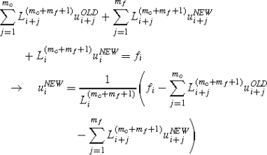  (79)

  In this case, when the MFD star consists of the larger number of the old nodes (m _f >1), additional techniques, e.g. smoothing, have to be applied. It is worth stressing that the formula (79) is quite suitable for effective iterative solution process.

Prolongation approach of the same type also holds for the variational formulation of b.v. problems δΠ(u ^OLD,u ^NEW)=0 as well. It may be introduced at each new node assuming the local variations δu ^NEW≠0 and δu ^OLD=0. Such an approach could be used not only in the MFDM, but also in the FEM.

6.2 Restriction

After the prolongation, the restriction is the second most important procedure in the multigrid solution approach. It will be discussed here in a new original form proposed and developed in [43, 64].

On the most fine cloud of nodes, one evaluates residuals

$$ r=Lu-f$$

(80)

however, instead of solving SLAE Lu=f, on that cloud of nodes evaluation of appropriate residuals for the subsequent coarser clouds is done, using the following assumptions [43, 64]:

• The “virtual work”

  $$ \delta W=\int_\varOmega{r\delta u} \,\mathrm{d}\varOmega $$

  (81)

  done by residuals r (residual forces) on the virtual displacements δu is the same for both the old and new clouds of nodes.

• Virtual displacements of new nodes δu ^NEW are found from the prolongation formula (77) determined above, namely

  $$ \delta u_i^{\mathit{NEW}} =\sum_j {\alpha_{ij} \delta u_j^{\mathit{OLD}} }$$

  (82)

One may evaluate appropriate MFD expressions of the virtual work on the new cloud of nodes, (83)

(83)

and on the old one (84)

$$ \delta W\approx\sum_c {\bar{r}_c^{\mathit{OLD}} \delta u_c^{\mathit{OLD}} \bar {\varOmega}_c^{\mathit{NEW}} }$$

(84)

where c∈I ^OLD, f∈I ^NEW.

Taking advantage of the linear independence of the virtual displacements $\delta u_{c}^{\mathit{OLD}}$ from each other, one may obtain the required relation between the residuals on the old cloud of nodes $\bar{r}_{c}^{\mathit{OLD}}$ and the residuals $r_{c}^{\mathit{NEW}}$, $r_{c}^{\mathit{OLD}}$ determined on the new cloud

(85)

(86)

In the above formulas, given are

• 1. residuals $r_{c}^{\mathit{NEW}}$, $r_{c}^{\mathit{OLD}}$ for new and old nodes of the new cloud,

• 2. surface areas of the Voronoi polygons $\varOmega_{c}^{\mathit{NEW}},\bar {\varOmega}_{c}^{\mathit{OLD}}, \varOmega_{f}^{\mathit{NEW}}$ for both the new and old clouds,

• 3. residuals $r_{f}^{\mathit{NEW}}$ and $r_{c}^{\mathit{OLD}}$ for new and old nodes of the new cloud.

6.3 Use of the Higher Order Correction Terms

In the standard MFD multigrid approach, raising order of local approximation was possible due to use of the so called HO MFD operators (Hackbush, [24]). They were built on larger number of nodes, or, more general, on larger number of degrees of freedom. The same multigrid solution algorithm was used in order to reduce the appropriate residual error, which appeared after applying such modified MFD operator.

In the HO approximation approach, proposed here, one does not need to generate new MFD operator. Instead of assuming new degrees of freedom, one has to consider appropriate correction terms of the same basic MFD operator, resulting from the Taylor series expansion of the sought function. Those terms modify the right hand side of the MFD residual defect, which may be reduced using the same prolongation and restriction procedures.

The approach involves two steps

• 1. First, residual error on the last fine cloud (with no HO correction) is considered, namely

  $$ r^{(L)}=L\bar{u}^{(L)}-f$$

  (87)

  where $\bar{u}^{(L)}$—is the prolonged solution from the previous clouds. When (87) is restricted to the basic cloud, it provides the appropriate correction Δu ^(L) of the prolonged solution $\bar{u}^{(L)}$.

  As the final result, one obtains the low order solution, which is exact for the considered fine cloud

  $$ u^{(L)}=\bar{u}{ }^{(L)}+\varDelta u^{(L)}$$

  (88)

• 2. Afterwards, when the low order solution u ^(L) (88) is obtained and the correction terms Δ ^(L)=Δ(u ^(L)) are evaluated, considered is improved form of the residual error (87), obtained by modification of its right hand side

$$ r^{(H)}=Lu^{(L)}-\varDelta { }^{(L)}-f$$

(89)

After substituting to residuum (89) the formulas (87) and (88), it may be simplified to the following form,

$$ \varDelta ^{(L)}=0$$

(90)

Here, the residual defect (90) comes directly from the HO correction, resulting from raising the approximation order, from p-th to 2p-th.

When the residual defect (90) is restricted to the basic cloud, it provides the appropriate HO correction Δu ^(H) of the low order solution (88). As the final result, one obtains the HO solution, which is exact for the 2p-th polynomial

$$ u^{(H)}=u{ }^{(L)}+\varDelta u^{(H)}$$

(91)

It is worth stressing, that the best quality Higher Order solution is usually required, only for the last, finest cloud of nodes. Therefore, an additional iterative solution smoothing of the Higher Order solution, corresponding to the (90), is not necessary on the intermediate clouds. For those clouds, one needs to apply the 3/2+3/2=3 of the multigrid cycle. In a particular case, the Higher Order solution is obtained only for the last cloud of nodes.

6.4 Non-adaptive Multigrid Solution Approach with HO Approximation

The above given concepts of the prolongation and restriction procedure are integral parts of the multigrid analysis. In the standard, non-adaptive, multigrid approach, one deals with the set of regular of irregular clouds of nodes, given a-priori. Usually, each new cloud contains all nodes of the old ones. However, this assumption does not hold, if nodes are removed from the subsequent clouds.

In the multigrid approach, the appropriate SLAE are solved only for the first, usually the coarsest cloud. The solution $\bar{u}^{(L)}$ is prolonged then step by step, to the last, finest cloud. After evaluating residuals (87) for that cloud, they are restricted to the first cloud, where the equivalent correction term Δu ^(L) is calculated. The final corrected solution (88), exact for the last cloud, is obtained when residuals for this cloud reach zero.

When the low order solution (88) is found, appropriate HO correction Δ ^(L) may be evaluated, resulting from additional terms of the Taylor series expansion of the MFD operator. The residual defect (90) is restricted again to the basic cloud of nodes, when the equivalent correction Δu ^(H) is calculated. The final HO solution (91), exact for the assumed approximation order, is obtained by means of correction prolongation.

The whole non-adaptive multigrid approach consists of the following steps

• 1. determination of a set of clouds, regular (meshes) or irregular ones,

• 2. generation of the nodes topology (in 2D: Voronoi polygons, Delaunay triangles) for all clouds,

• 3. selection of MFD stars for all clouds,

• 4. generation of the MFD formulas for Du (complete set of low order derivatives) and Lu by means of the MWLS approximation for all clouds; use of these formulae for composition of difference operator, corresponding to the differential operators, appearing in the boundary value problem formulation,

• 5. derivation of the Higher Order correction terms, Δ, corresponding to the Du and Lu for the last cloud only,

• 6. generation of the MFD equations, depending on the problem formulation, for all clouds

• 7. imposing of the boundary conditions, for all clouds

• 8. solution of Lu ^(L)=f for the basic cloud, and obtaining the low order solution u ^(L),

• 9. evaluation of the correction terms Δ, for the basic cloud,

• 10. solution of Lu ^(H)=f−Δ ^(L) equation for the basic cloud, and obtaining the Higher Order solution u ^(H),

• 11. prolongation of the solution $\bar{u}^{(L)}$ through the intermediate clouds to the last cloud, e.g. in the case, when the MFD star, used for prolongation, contains only one new node

  • • prolongation formula for the new nodes in the new cloud,

    

    (92)

  • 12. prolongation formula for the old nodes (common for two clouds).

    $$ u_i^{\mathit{NEW}} =u_i^{\mathit{OLD}},\quad i=0,1,\ldots,n^{\mathit{OLD}}$$

    (93)

  The above given explicit formulae hold only for the simplest case, when each MFD star consists only one new node. However, MFD star, built in such way, are of worse quality than the ones using additional new nodes. The problem becomes implicit one then and should be treated in an iterative way.

  The above formulas may be presented in the matrix notation

  $$ u^{\mathit{NEW}+\mathit{OLD}}=M\cdot u^{\mathit{OLD}}+f$$

  (94)

  where M is the prolongation matrix

  

  (95)

• 12. optional smoothing steps for intermediate clouds and residual calculation on the last cloud

  $$ r^{(L)}=L\bar{u}^{(L)}-f$$

  (96)

• 13. residuum restriction to the basic cloud.

  Restriction formula for the new nodes in the new cloud

  

  (97)

  may be written in the following matrix notation

  $$ r^{\mathit{OLD}}=R\cdot r^{\mathit{OLD}+\mathit{NEW}}$$

  (98)

  where R is the restriction matrix

  

  (99)

• 14. solution correction term Δu ^(L) calculation for the basic cloud

  $$ L\left( {\varDelta u^{(L)}} \right)=r$$

  (100)

• 15. prolongation of the correction Δu ^(L) through the intermediate clouds to the last cloud

  $$ \left( {\varDelta u^{(L)}} \right)^{\mathit{NEW}+\mathit{OLD}}=M\left( {\varDelta u^{(L)}}\right)^{\mathit{OLD}}+r$$

  (101)

• 17. the final correction of the low order solution for the last cloud,

  $$ u^{(L)}=\bar{u}^{(L)}+\varDelta u^{(L)}$$

  (102)

• 18. evaluation of the correction terms for the last cloud

• 19. optional smoothing steps, residual calculation

  $$ r^{(H)}=Lu^{(L)}-\varDelta ^{(L)}-f$$

  (103)

• 20. repetition of the steps (xiii)–(xv) for the residuum r ^(H)

• 21. the final correction of the Higher Order solution for the last cloud

  $$ u^{(H)}=\bar{u}^{(H)}+\varDelta u^{(H)}$$

  (104)

• 1. postprocessing of final results, on the last cloud.

The above given algorithm for the non-adaptive solution approach, may be illustrated in the following diagram (Fig. 13). For the sake of simplicity, smoothing iteration steps are omitted here, following the assumptions that prolongation formulas are found using MFD stars with one new node only.

Fig. 13

Non-adaptive multigrid solution path for HO MFDM

6.5 Adaptive Multigrid Solution Approach with HO Approximation

As opposite to the non-adaptive multigrid solution approach with the HO approximation considered above, adaptivity is applied here [64]. Solution procedure is combined with simultaneous design of subsequent clouds of nodes. It is based on the results of an a-posteriori error analysis, especially on the improved estimation of the true residual error. Therefore, sufficiently precise Higher Order solution is needed not only on the finest cloud, but also on all intermediate ones. This solution is applied then to Higher Order estimation of the residual error at points being the candidates for insertion of new nodes.

The following steps of the general solution approach are needed then

• 1. design and generation of an initial (basic) coarse cloud,

• 2. generation of the cloud topology (Voronoi polygons, Delaunay triangles in 2D), for the current cloud,

• 3. selection of MFD stars for this cloud

• 4. generation of the MFD formulas Du (complete set of low order derivatives) by means of the MWLS approximation; use of these formulae for composition of Lu (a difference operator, corresponding to differential operators, appearing in the boundary value problem formulation),

• 5. derivation of the Higher Order correction terms, Δ, corresponding to the Du and Lu, for the current cloud,

• 6. generation of the MFD equations, for the current cloud, depending on the problem formulation,

• 7. imposing of the boundary conditions for the current cloud,

• 8. solution of Lu ^(L)=f for the basic cloud, and obtaining the low order solution u ^(L), exact for that cloud,

• 9. evaluation of the correction terms Δ, for the basic cloud,

• 10. solution of Lu ^(H)=f−Δ ^(L) for the basic cloud, and obtaining the Higher Order solution u ^(H), by means of the HO solution smoothing,

• 11. one level denser cloud generation, with proposed localisation of new nodes,

• 12. generation of the MFD operators Lu and derivation of the Δ terms at points being candidates for new nodes insertion,

• 13. a-posteriori residual error evaluation r ^(H)=Lu ^(H)−Δ ^(H)−f at points being candidates for new nodes insertion, and acceptance of those, where residual error exceeds its admissible value ∥r ^(H)∥≥η _adm ; additional nodes generation criteria may be also applied and satisfied here,

• 14. solution $\bar{u}^{(L)}$ prolongation to the new cloud, in a way depending of number on the new nodes in the MFD star; simple explicit formula (78) may be used in the case when the MFD star consists of one new node only; smoothing iterations may be needed, if the MFD star contains more than one new node (79),

• 15. optional smoothing steps and residual error calculation $r^{(L)}=L\bar{u}^{(L)}-f$ for the new cloud,

• 16. residuum r ^(L) restriction to the basic cloud,

• 17. solution correction calculation L(Δu ^(L))=r ^(L) for the basic cloud,

• 18. solution correction Δu ^(L) prolongation to the new cloud,

• 19. final correction of the low order solution u ^(L) for the new cloud,

• 20. evaluation of the correction terms Δ ^(L) for the new cloud,

• 21. optional smoothing steps and residual error calculation r ^(H)=Lu ^(L)−Δ ^(L)−f,

• 22. repetition of the steps (xvi)–(xviii) for the residuum r ^(H),

• 23. final correction of the Higher Order solution u ^(H) for the last cloud,

• 24. repetition of steps (xxi)–(xxiii) until convergence is reached,

• 25. repetition of steps (xi) – (xxiv) until sufficient solution precision ∥r ^(H)∥≥η _adm is reached in the proposed new nodes locations of the next cloud (corresponding to the step (xiii)),

• 26. final postprocessing of the results performed on the last cloud.

The above proposed solution steps may be also presented in the form of the adaptive solution path (Fig. 14). Here, for the sake of simplicity, smoothing iterations are omitted. They may be needed, if the MFD star, used in prolongation procedure, contains more than one new node. However, smoothing iterations may be performed simultaneously with the HO iterations, improving the HO solution. The whole algorithm of the multigrid adaptive solution approach with the HO approximation is presented in the form of the flow chart in Fig. 15.

Fig. 14

Adaptive multigrid solution path for HO MFDM

Fig. 15

Flow chart of the adaptive multigrid solution approach with the HO approximation

7 Numerical Examples

A variety of benchmark tests of 1D and 2D boundary value problems were solved so far using the higher order approximation technique. Many aspects of the proposed approach were tested. Mostly the following ones were investigated:

• application of the approach to the local solution and residual error estimation, when using higher order terms,

• application of the approach to the global estimation of the solution error when using various types of global estimators and higher order terms,

• application of the higher order estimators to an appropriate adaptive cloud of nodes generation,

• examination of the error indicators, convergence rate and solution quality improvement on those clouds,

• reduction of the calculation time, when using the HO multigrid adaptive strategy, based upon a-posteriori error estimation.

Finally, the MFDM solution approach with the Higher Order terms was applied in analysis of selected engineering problems.

7.1 Introductory 1D Example

1D example shows the main idea of the proposed approach. A simply supported beam under uniform loading is considered (Fig. 16). For the case of simplicity, the boundary value problem is posed in the local formulation

(105)

where M(x) denotes bending moment, EJ—bending stiffness, 2l—beam length, and q—uniform load. The most rough discretization with only 3 regularly spaced nodes is used, (with modulus h=l). Therefore, only one unknown function value w ₁ appears.

Fig. 16

1D introductory example—simply supported beam under uniform load

Standard (second order) difference operator is applied $w_{1}^{\mathit{II}} \approx Lw_{1} =\frac{w_{0} -2w_{1} +w_{2} }{l^{2}}$. By collocation in the central node, Lw ₁=f ₁, and after providing boundary conditions w ₀=w ₂=0, one gets the difference solution, which is of the low order (corresponds to the low order difference operator L).

$$ \begin{cases}Lw_1 =f_1 \\w_0 =w_2 =0 \\\end{cases}\Rightarrow\quad w_1^{(L)}=\frac{1}{4}\frac{ql^4}{EJ}$$

(106)

Expansion of the function values of the difference operator Lw ₁ into the Taylor series

(107)

yields the form of the considered correction terms Δ ₁ (derivatives up to the 4-th order) and the neglected truncation error R ₁. The value of the higher order derivative $w_{1}^{\mathit{IV}}$ is calculated using formula composite, like

(108)

and low order solution values

(109)

The correction term $\varDelta _{1} =-\frac{1}{12}ql^{2}$ modifies the right hand side of the difference equation (106) (Lw ₁=f ₁−Δ ₁), whereas the difference operator L remains unchanged. Solution of this modified equation yields the higher order solution

$$ \begin{cases}Lw_1 =f_1 -\varDelta _1 \\w_0 =w_2 =0 \\\end{cases}\Rightarrow\quad w_1^{(H)}=\frac{5}{24}\frac{ql^4}{EJ}$$

(110)

which is exact within the 4-th polynomial order. In fact, it is the exact analytical solution as well, because in this case the beam deflection is described by the polynomial of the 4-th order (R ₁=0). Thus the exact solution is obtained using only one node with the unknown value.

The above example, though very simple, reflects the main concept and advantages of the Higher Order approach. The whole procedure needs two steps only, with the same difference operator, but with modified right hand side. The final Higher Order solution suffers from the truncation error (here, R=0), but does not depend on the quality of the difference operator used in the first step.

7.2 Beam Buckling Example

This benchmark was chosen mainly for

• Examination of the quality of the HO solution, in the case when the analytical solution is described by a non-polynomial function (here trigonometrical),

• Comparison of the true analytical errors of both the low order and HO solutions,

• Examination of the convergence rates and solution convergence improvement on the set of regular clouds.

Formulation of the boundary value problem, which can be treated as eigenvalue problem of the differential equation

(111)

The classic Euler problem was also solved using either the low order or higher order approximation in order to examine the quality of those solutions, as compared to the exact value of the Euler force

$$ P_E =\frac{1}{4}\frac{\pi^2EJ}{L^2}\approx2.467\frac{EJ}{L^2}$$

(112)

Considered was the coarse regular mesh with 2 nodes only (spaced with h=L). Discretization of the natural condition w′(0)=0 was performed using a fictitious node f and evaluation

$$ w_0' \approx\frac{w_1 -w_f }{2h}=0\quad\Rightarrow\quad w_f =w_1$$

(113)

Classical FD operator for the second derivative

$$ w''_i \approx\frac{w_{i-1} -2w_i +w_{i+1} }{h^2}$$

(114)

was used for the internal nodes. For the mesh shown in (Fig. 17) (one nodal unknown w ₁= ?), the following FD solutions (values of buckling forces) are obtained together, with the appropriate exact relative error

$$ \varepsilon=\biggl| {\frac{P-P_E }{P_E }} \biggr|\times100\%$$

(115)

• Low order solution (mesh with 2 nodes, Fig. 17) $P_{\mathit{LO}}=2\frac{EJ}{L^{2}}$, ε _LO =18.9%,

  Fig. 17

  

  Cantilever beam subjected to buckling load P

• Higher order solution (mesh with 2 nodes, Fig. 17) $P_{\mathit{HO}} =2.40\;\frac{EJ}{L^{2}}$, ε _HO =2.7%.

Precision of the higher order solution is over 6 times better than the lower order one. Calculations for the set of ten regular more and more dense meshes were performed, showing that the quality of the low order solution on the last mesh (with 11 nodes) is similar to the higher order one on the second mesh with 3 nodes only (Fig. 18). Furthermore, the convergence rates, evaluated in the logarithmic scale a _LO =1.94, and a _HO =4.03 yield solution convergence improvement $\frac{a_{\mathit{HO}} }{a_{\mathit{LO}} }=2.08$, which means that the HO error ε _HO decreases over 10²=100 times faster, when compared with the low order one ε _LO . The dashed line in Fig. 18 represents the true LO solution error level for mesh with 13 nodes. In this simple case, the same true HO error level may be achieved for the mesh with 3 nodes only.

Fig. 18

Convergence of the LO and HO FD solutions for the 1D buckling problem

7.3 2D Boundary Value Test Problem

The boundary value problem described by the Poisson equation with the essential boundary conditions

(116)

was analysed (w∈C ²). The following exact solution was considered [28]

(117)

shown in Fig. 19 with the right hand side function. The appropriate variational weak (Galerkin) form was analysed as well ($w\in H_{0}^{1}$, $\forall v\in H_{0}^{1} )$

(118)

Regular mesh with 400 nodes only was used for calculations. Results for both the local and global (variational) formulations are presented in Fig. 20 (local) and Fig. 21 (variational). In those figures, the first row presents plots (in the same scale) of the low order local solution error e ^LT, Higher Order local solution error e ^HT and Higher Order local estimation of the low order local error e ^LH respectively. Their second rows present the true local residual error r ^t, its low order local estimation r ^L and Higher Order (improved) local estimation r ^H, respectively.

Fig. 19

Exact solution and right hand side function for the 2D test

Fig. 20

Local solution and residual error estimations—local formulation

Fig. 21

Local solution and residual error estimations—variational formulation

The same mesh was used for comparison of the chosen global estimators of the low order solution error of (116). The estimators were evaluated between nodes, on the Delaunay triangles (one integral value over each triangle), and over the whole domain (one value for the whole domain). They are presented (Figs. 22 and 23) starting from the exact error distribution. Then hierarchic estimators (p, h, HO), smoothing (Z-Z, HO) and residual (explicit and implicit) are presented. Above the graphs, the effectivity indexes (71) values are given. The best results were obtained when using the Higher Order hierarchic estimator (i=1.03) and Higher Order smoothing estimator (i=1.23). Their quality is superior, especially when compared to the other ones.

Fig. 22

Global solution error estimation: exact error; h-hierarchic, p-hierarchic and HO hierarchic estimators

Fig. 23

Global solution error estimation: ZZ-smoothing, HO-smoothing, residual explicit and residual implicit estimators

Further tests concerned application of higher order estimators to an appropriate adaptive nodes generation. First, the coarse regular mesh with 16 nodes was given. The subsequent clouds were generated using the criteria (72)–(73), and the local estimation of the residual error (39) of (116). The adaptation process was stopped after 60 iterations (Fig. 24), when the break-off criterion was satisfied. The final finest, strongly irregular cloud consisted of 179 nodes. During the adaptation process, the representative pairs $(\bar{h},\bar{e})$ had been calculated on each cloud separately, using simple (centre of gravity) error indicator (75). Those quantities were used in order to examine the convergence of the solution and residuum on the set of irregular adaptive clouds. The convergence rates (Fig. 25), for the low order solution (the blue dots) a ^(L)=2.01 and for the higher order one (the red dots) a ^(H)=4.29 give the final solution improvement rate (in the logarithmic scale) a ^(H)/a ^(L)=2.37. The corresponding residuum improvement reaches a ^(H)/a ^(L)=2.47.

Fig. 24

Set of irregular adaptive clouds of nodes

Fig. 25

(Color online) Solution and residual convergences on the set of irregular clouds

Above mentioned values of convergence rates are collected in Table 1. They are compared there with the values of convergence rates obtained for the sets of regular meshes, with the similar number of nodes as it appears in the appropriate irregular cloud. Though the HO convergence are very high (however similar to those obtained for irregular clouds), the improvement rates are not as high as in the irregular case. MFD operators are much more precise than for the irregular clouds. However, the improvement rates for irregular clouds appear to be much higher—in such case the low order MFD (without correction terms) is rather of low quality and it requires a lot of individual adjustment. On the other hand, similarity in convergence rates for both regular and irregular cases proved the HO MFD solution to be independent from the quality of the basic low order MFD operator.

Table 1 Comparison of the low and Higher Order solution and residual convergence rates, evaluated on the sets of regular meshes and adaptive irregular clouds of nodes

Finally, the comparison of the solution time between the standard (without multigrid) and the multigrid solution approaches was investigated. Two various situations were examined: HO multigrid approach on regular meshes (Fig. 26), and adaptive HO multigrid approach (Fig. 27) for the set of clouds of nodes already presented in Fig. 24.

Fig. 26

Comparison of computational time for the HO standard and HO adaptive multigrid solution approaches for regular meshes

Fig. 27

Comparison of computational time for the HO standard and HO adaptive multigrid solution approaches for irregular clouds

In each case multigrid approach speeded up the FD analysis. Results show potential power of the multigrid approach in order to reduce the computational time involved in the analysis of large boundary value problems.

In the case of regular meshes (non-adaptive multigrid solution approach) tested the speed up factor for the solution time was

$$ T=\frac{t_{\mathit{STANDARD}} }{t_{\mathit{MULTIGRID}} }=45.69$$

(119)

and in the case of irregular clouds of nodes (adaptive multigrid solution approach) the speed up factor for the solution time was

$$ T=\frac{t_{\mathit{STANDARD}} }{t_{\mathit{MULTIGRID}} }=10.12$$

(120)

One should realise that the solution time, in case of multigrid approach, strongly depends on the software and hardware type used. Effective implementation of the algorithms as well as use of parallel computing may additionally increase the speed up factors (119) and (120). Moreover, significant achievement of solution time is specially expected when dealing with larger numbers of unknowns.

8 Selected Engineering Applications

The MFDM approach may be used in variety of engineering applications. Selected 1D and 2D problems present some chosen examples of such numerical analysis. Especially, the railroad rail analysis, presented here, may be treated as part of larger research, focused on the analysis of the residual stresses [30, 34, 73, 86]. Those simple tests give hope how much could be gained towards effective solving more sophisticated 2D and 3D problems, when using the MFDM with HO approximation.

In the first tests, solved are simple non-linear b.v. problems. However, the main goal of these tests is to present the possibility of the HO correction terms integration into the standard iterative solution approach of a non-linear problem. Moreover, the successive over-relaxation method is applied, in order to speed up the iteration process. New concepts of evaluating the relaxation parameter are proposed [84, 88]. They are expected to provide the significant solution convergence and calculation time improvement, when compared with the standard acceleration techniques. The following tests are 1D problems of rather simple nature as well. However, the discrete analysis of those tests requires multiple solving of boundary value problems. Therefore, effective and fast numerical tool is needed.

8.1 Formulation of the HO MFDM Solution Approach for the Non-linear Problems

The non-linearity in mechanics [50, 101] may have two main sources, namely geometrical (e.g. large deformations, large strains) and physical ones (e.g. non-linear constitutive law). In the present section, the general MFDM solution approach for analysis of the non-linear boundary value problems is presented. The quality of the MFD approximation may be raised by considering HO correction terms. Those terms are involved in the standard MFD iterative solution approach, applied in the case of non-linear problems. Proposed is also a new concept of acceleration of the standard Newton-Raphson method [99], used for iterative solution of the Simultaneous Algebraic Equations (SAE).

Consider the locally formulated boundary value problem

$$ \begin{cases}Lu=f&\mbox{in }\varOmega\\L_b u=g&\mbox{on }\partial\varOmega \end{cases}$$

(121)

For linear problems, the differential operator L may be presented in the form

$$ L(u)=a_0 u+a_1 u_x +a_2 u_y +a_3 u_{xx} +\cdots $$

(122)

with functional coefficients a _i =a _i (x), i=0,1,… . The MFDM discretization leads to the Simultaneous Linear Algebraic Equations (SLAE) then. Such group of problems was considered in the previous chapters.

For the non-linear problems, the differential operator L may be presented in the following general form

$$ L(u)=F\biggl(u,\frac{\partial u}{\partial x},\ldots,\frac{\partial ^{(p)}u}{\partial x^{(p)}}\biggr)$$

(123)

Solution of (121) may be obtained then by the method of successive iterations, solving the appropriate SLAE on every step of calculations.

In the most primitive method of simple iterations, one solves the linear problem, corresponding to (121) and (123), in which the derivatives values $u,\frac{\partial u}{\partial x},\ldots,\frac{\partial^{(p-1)}u}{\partial x^{(p-1)}}$ are evaluated from the previous iteration step. However, convergence of this method may be poor or not sufficiently fast.

Much faster are those methods, in which the values obtained from the SLAE are treated as the correction terms, added to the unknown function u. Among them, one may distinguish Newton-Raphson method and its numerous modifications. Their common feature is using of the tangent (or secant) incremental matrix, while they differ from each other in the manner of calculating the right hand sides of the SLAE. The incremental matrix $\frac{\partial F}{\partial u}$ is derived from the Taylor series expansion of (123) with respect to the unknown function u

$$ L(u)=F_0 +\frac{\partial F}{\partial u}\varDelta u+\cdots\approx F_0+\frac{\partial F}{\partial u}\varDelta u$$

(124)

where Δu—corrections of the solution, and F ₀—result of the previous iteration step. In the Newton-Raphson method, the right hand side of the SLAE comes from the difference between the function f of the differential equation (121) and the current value of the left hand side of (121). The initial approximation is improved, during the iteration process, until the final precision is reached.

In the practical applications, the Newton-Raphson method is combined with the incremental approach, where the total non-homogeneity of the system is divided into n (n>0) increments (e.g. load increments). For each increment, the iterative Newton-Raphson is applied separately. Moreover, additional acceleration of the convergence may be obtained by using appropriate relaxation or the self-correcting approach. The general incremental Newton-Raphson method with the correcting parameter α (α=1.2–1.3) [45] may be given in the following form

$$ \varDelta u_i \frac{\partial F}{\partial u}=\frac{i\cdot f}{n}-\alpha\biggl({\frac{i\cdot f}{n}-F_{i-1} } \biggr),\quad i=1,2,\ldots,n$$

(125)

where $\frac{\partial F}{\partial u}$ is the incremental Jacobian matrix (124), n—assumed number of increments, F _i−1—left hand side value of (121), on the previous iteration step. The geometrical interpretation of (125) for 1D case is shown in Fig. 28.

Fig. 28

Incremental Newton-Raphson method with the selfcorrecting approach

Evaluation of the incremental matrix (124) may be performed in several ways. Among them one may distinguish

• 1. N-R method with the tangent incremental matrix, evaluated using analytical methods,

• 2. N-R method with the secant incremental matrix, evaluated using numerical differentiation,

• 3. Modified N-R, in which the incremental matrix is updated after several iteration steps,

• 4. Initial NR, in which the incremental matrix is evaluated once for each increment,

• 5. N-R method, in which the incremental matrix has the diagonal form.

In the MFDM analysis, symbolic derivation may be used for evaluating the tangent matrix on every k-iteration step [37, 38, 45, 97], followed by application of the MFD formulas, generated by the means of the MWLS approximation,

(126)

Here differentiation $\frac{\partial F_{j} }{\partial u_{i}^{(s)}}$, s=0,1,…,p may be performed analytically, by symbolic operations, while derivatives $\frac{\partial u^{(s)}}{\partial u_{j} }$, s=0,1,…,p come from an appropriate MFD formulae, generated and composed for the set of partial derivatives, at the basic stage of the approach. This approach was successfully applied in several systems, designed for the discrete analysis of the boundary value problems (e.g. FIDAM [45] and NAFDEM [36, 38]).

In the present paper, the approach is used together with a new concept of acceleration of the NR convergence. Instead of using self-correcting method, with arbitrarily chosen coefficient α, the modified relaxation technique is proposed.

In the most iterative methods, for both the SAE and SLAE, the constant relaxation parameter μ is chosen in such a way as to minimise the spectral radius of the error dumping matrix [90]. Evaluation of such μ is difficult, so it is obtained approximately, based on trial and error values of μ and observing the convergence (μ=1.2–1.4). In the proposed optimal relaxation method (Fig. 29), proposed by Orkisz [88], and developed by Orkisz and author of the present paper [84], the variant relaxation parameters μ ^(k) or μ ^(k),λ ^(k) are chosen in such a way that they minimise the relaxed residuum magnitude of the current solution $\hat{u}^{(k)}$.

(127)

The relaxation parameter(s) is/are variable. In each iteration step their values are found by means of simple calculations. Two situations may be distinguish

• 1. one relaxation parameter μ ^(k) is found by minimising the magnitude I of relaxed residuum r ^(k) of current solution

  

  (128)
  

  (129)
  

  (130)

  Fig. 29

  

  Search for the optimal relaxation

• 2. two relaxation parameters μ ^(k) and λ ^(k) are found after two iteration steps by minimising the modified residuum functional

  

  (131)

  hence

  $$ \begin{cases}\mu^{(k)}=-\frac{( {r^{(k-1)} } )^t\varDelta r^{(k-1)}-\frac{( {\varDelta r^{(k)} } )^tr^{(k-1)} }{( {\varDelta r^{(k)} } )^t\varDelta r^{(k-1)} }( {\varDelta r^{(k-1)} })^t\varDelta r^{(k-1)} }{( {\varDelta r^{(k)} } )^t\varDelta r^{(k-1)} -\frac{( {\varDelta r^{(k)} } )^t\varDelta r^{(k)}}{( {\varDelta r^{(k)} } )^t\varDelta r^{(k-1)} }( {\varDelta r^{(k-1)} } )^t\varDelta r^{(k-1)} } \\[12pt]\lambda^{(k)}=-\frac{( {r^{(k-1)} } )^t\varDelta r^{(k-1)}+\mu ^{(k)}\cdot( {\varDelta r^{(k)} } )^t\varDelta r^{(k-1)} }{({\varDelta r^{(k-1)} } )^t\varDelta r^{(k-1)} } \\\end{cases}$$

  (132)

  and finally

  

  (133)

As it was shown in [84, 88], the relaxation discussed above may significantly raise the convergence rates of the iterative methods, and reduce the computational time.

The convergence of the N-R iterative method should be controlled by estimating both the solution and residual errors

(134)

Here, ε _adm and ω _adm denote the admissible error values, for solution and residuum respectively.

In the MFDM solution approach, the non-linear analysis is integrated with the solution process. One may combine here the features of iterative procedures of the Newton-Raphson method (125) and smoothing of the HO solution. Both methods deal with the same coefficient matrix of the set of MFD equations, both with a modified right hand side vector. Their modification may include here

• 1. corrections derived from the NR method

  $$ \delta_{ij}^{(k)} =F_{u_j } \bigl( u_i^{(k-1)},\ldots, ( {u_i^{(p)} })^{(k-1)}\bigr)\cdot u_j^{(k-1)} -f_i^{(k-1)}$$

  (135)

• 2. optimal relaxation of the solution, with use of one parameter, or two parameters

• 3. Higher Order corrections derived from the Taylor series expansion of the MFD operator value

  $$ \varDelta _{ij}^{(k)} =\varDelta _{ij}^{(k)} \biggl( {\frac{\partial ^{(p+1)}u}{\partial x^{(p+1)}},\ldots,\frac{\partial^{(2p)}u}{\partial x^{(2p)}}} \biggr)$$

  (136)

  evaluated by means of the appropriate formulae composition.

The rough derivatives, derived from the MWLS approximation without correction (136), are evaluated only for the first iteration of the N-R algorithm. On the next iterative steps, each MFD formula is improved by its appropriate corrections, which are consequently added to the right hand sides of the SLAE. Higher Order derivatives values (136) are upgraded in the same time as the corrections (135) are getting smaller and smaller. The convergence is controlled by the (134) criteria.

8.2 Large Deflections of the Cantilever Beam

Considered was large deflections problem of the cantilever beam, loaded with a concentrated moment M and, in what follows, with a concentrated force P. The boundary value problem, posed in the local formulation

(137)

was transformed to the form, using the parametric notation x=x(s), w=w(s), shown in Fig. 30. This transformation was performed in order to allow very large for beam deflection analysed in all four sectors of the co-ordinate system (s∈〈0,2π〉).

Fig. 30

Cantilever beam with large deflections

The parametric co-ordinates

$$ \mathop {x}^\bullet=\frac{\mathrm{d}x}{\mathrm{d}s},\qquad\mathop {w}^\bullet =\frac{\mathrm{d}w}{\mathrm{d}s}$$

(138)

allow for evaluating derivatives required in the differential equation (137)

(139)

Therefore, the curvature, which appears in (137), may be presented in the following parametric form

(140)

After simplifying the denominator of (140)

(141)

one obtains the parametric notation of the beam deflection problem for large deformations, equivalent to the form (137)

(142)

where $f(x,w)=-\frac{M(x,w)}{EJ}$. Additional conditions are applied on the boundary

$$ w(0)=0,\qquad w'(0)=0,\qquad x(0)=0$$

(143)

Moreover the beam preserves the constant length L

$$ \int_0^L {\mathrm{d}s=L} \quad\to\quad \int_0^L {\sqrt{{\mathop {x}^\bullet}^2+{\mathop {w}^\bullet}^2} \,\mathrm{d}s=L}$$

(144)

during the whole deformation process.

Regular mesh with 20 nodes was introduced for the test with the concentrated moment $f(M)=\frac{M}{EJ}$ at the unbounded end of the beam, with L=1. Calculations were performed according to the MFDM solution algorithm, proposed in the previous sections. However, the adaptive approach was not applied here. The load was successively increased, following the subsequent deformation forms of the beam. The mesh remained unchanged. Results are presented in Fig. 31. It is worth stressing the quality of the solution represented by the ideal circle despite how large the deflection is.

Fig. 31

Large deflections of the cantilever beam under concentrated moment—non-adaptive HO MFDM solution approach

More sophisticated test deals with beam loaded by the concentrated following force. The following form of the right hand side function may be written then

$$ f(x,w,P)=\frac{1}{EJ}\left[ {P_X (w_L -w)+P_Y (x_L -x)} \right]$$

(145)

where P _X and P _Y are load projections in the ‘x’ and ‘y’ axis, respectively. The full MFDM algorithm with adaptation and HO approximation, proposed in the previous section, was applied here.

Each time the mean residual error

$$ r_x =\sqrt{\left( {\mathop {w}^{\bullet\bullet} -f\cdot\mathop {x}^\bullet} \right)^2+\left( {\mathop {x}^{\bullet\bullet}+f\cdot\mathop {w}^\bullet} \right)^2}$$

(146)

evaluated at the points between two neighbouring nodes, was larger than the admissible threshold value ε _adm =0.01, the cloud of nodes was refined by means of inserting new nodes. Additionally, the set of clouds was analysed using the multigrid technique, discussed in the previous section. Therefore, each time the appropriate SLAE was solved on the very first coarse regular mesh with 5 nodes only, constituting 4 unknown parameters (nodal deflections).

The results are presented in Fig. 32. In the initial state, the basic regular mesh with 5 nodes only, was introduced. Despite inserting new nodes into the mesh (becoming irregular cloud now), during the deformation process, the residual error (146) raised, because of the increased load value. As a consequence, new nodes were again added. Therefore, the residuum (146) was kept each time on the same threshold level ε _adm =0.01.

Fig. 32

Large deflections of the cantilever beam under concentrated following force—adaptive multigrid HO MFDM solution approach

8.3 Reliability Estimation

Another example was also chosen to show the area of application of the MFDM approach, as the effective and precise numerical tool. The reliability estimation problem for the simple 1D structure will be analysed [32, 66]. In mechanics, reliability is understood as probability of situation when failure, due to appropriate criterion, does not appear. For the simply supported beam, presented in Fig. 33, given is the probability distribution of the concentrated force location p(x).

Fig. 33

Safe and failure locations, due to the probability distribution

The force location may fall into the safe Ω _s or failure Ω _f zones. The force locations in the failure zones Ω _f produce non-admissible solutions, for beam deflections, violating the applied criterion

$$ g=w_{\mathit{adm}} -w_{\max} \ge0$$

(147)

Here w _max is the maximum beam deflection caused by the fixed force location, and w _adm —admissible deflection (Fig. 34) given. Therefore, the probability of failure may be defined, as follows

$$ P=\frac{\int_{\varOmega_f } {p(x)} \cdot \mathrm{d}\varOmega_f}{\int_{\varOmega_f +\varOmega_s } {p(x)\cdot \mathrm{d}\varOmega} }$$

(148)

and the reliability is the probability of the reverse situation

$$ R=1-P$$

(149)

Fig. 34

Admissible and non-admissible solutions

In the discrete analysis, applied here reliability of a considered beam was estimated using the Monte Carlo simulation method, and the MFDM solution approach. In the Monte Carlo simulation method [17, 59], one deals with many force locations, randomly chosen, due to the probability distribution. For each fixed location the beam deflection problem is solved using the MFDM approach. The failure criterion is checked, and the load configuration is examined then, whether it results in safe or failure solution. The probability of failure and reliability may be estimated, as follows

(150)

here n _f denotes the number of failure locations and n _s —number of safe locations, derived from the Monte Carlo simulations and MFDM solutions. The large number of random solution needed requires fast tool for solving the boundary value problems with sufficiently high precision.

The above proposed solution approach, using the Monte Carlo simulation method [17], and the HO MFDM solution approach, is given below

• 1. assume the admissible beam deflection u _adm , used in the failure criterion,

• 2. choose a random force location on the beam, based to the Gaussian type probability distribution p(x)

• 3. for fixed force location, solve the boundary value problem

  

  (151)

  using the HO MFDM approach, and randomly chosen loading data

  Details of the MFDM solution approach

  • beam was discretized with 33 nodes, regularly spaced,

  • solution approach included the MFD schemes generation by means of the MWLS approximation, HO approximation using correction terms, as well as an improved a-posteriori error estimation,

  • cloud of nodes refinement in the closest neighbourhood of the boundary and force,

• 4. find the maximum nodal value of beam deflection u _max,

• 5. check, whether the failure criterion (147) is satisfied, if not, increase the number of failures n _f ,

• 6. finally, estimate the beam reliability (150).

In Fig. 35, presented is the exemplary result of the random procedure, with the force location fixed, as well as the beam deflection problem solved, and failure criterion checked. The force was located in the failure zone, in this case.

Fig. 35

Exemplary Monte Carlo simulation with the MFDM analysis

The tests were performed in 100 series, each one consisted of 2,000 Monte Carlo simulations. That gives the total number of solved boundary value problems equal to 200,000. The final results are presented in Fig. 36. Shown are

• 1. the exact reliability value, evaluated using formulae (148) and (149)—dashed line,

• 2. numerical estimation of the reliability (150), from one of the 100 series—light thick line,

• 3. numerical estimation of the reliability (150), averaged from all 100 series—dark thick line.

Fig. 36

Reliability estimation convergence

High convergence rate may be observed, when the averaging method is applied. The final numerical results are very close to the theoretical value of beam reliability.

The above given 1D examples, though of very simple nature, shows, that there is still need for exploring new solution methods, and developing the existing ones. Analysis of many sophisticated problems of mechanics may be easier and faster then.

8.4 Stationary Heat Flow Analysis in the Railroad Rail

The stationary heat flow in 2D domain will be considered. The locally formulated boundary value problem may be posed in the form of the differential equation of the second order with the appropriate boundary conditions of essential and natural type

$$\everymath{\displaystyle}\begin{cases}-k_x \frac{\partial^2T}{\partial x^2}-k_y \frac{\partial^2T}{\partial y^2}=f& \mbox{in}\ \varOmega\\-k_n \frac{\partial T}{\partial n}=\bar{q}_n&\mbox{on}\ \partial\varOmega_q \\T=\bar{T}&\mbox{on}\ \partial\varOmega_T \\\end{cases} $$

(152)

Here:

• Ω, ∂Ω=∂Ω _q +∂Ω _T are the problem domain and its boundary,

• T=T(x,y) is the sought temperature function,

• k _x ,k _y are known values of the coefficients of thermal conductivity,

• f=f(x,y) is the known function of the heat generation inside the domain,

• $\bar{q}_{n}$ is the known function of the heat flux on the boundary Ω _q ,

• $\bar{T}$ is the known temperature function on the boundary Ω _T .

• n=(n _x ,n _y ) is the versor normal to the boundary.

The appropriate variational problem concerns determination of such a temperature function $T\in H_{0}^{1} +u(\bar{T})$, which fulfils the essential boundary conditions from (152), that for any $\forall V\in H_{0}^{1}$ satisfied is the following principle

(153)

The above given problem was analysed by means of two different discrete approaches, namely the HO MFDM using the local formulation (152) as well as the standard Finite Element discretization and approximation approach applied to the variational principle (153). The HO MFDM solution approach consists of two steps, for low order (standard second order approximation inside the domain) and higher order solution (fourth order approximation, provided by the correction terms of the second order difference operators). The appropriate MFD equations may be given in the following forms

• for the low order solution

  $$ \everymath{\displaystyle}\begin{cases}-k_x \sum_{j=1}^r {M_{4,j} T_{j(i)} } -k_y \sum_{j=1}^r{M_{6,j} T_{j(i)} } =f_i \\\quad \mbox{in}\ P_i \in\varOmega\\-k_x n_x \sum_{j=1}^r {M_{2,j} T_{j(i)} } -k_y n_y\sum_{j=1}^r {M_{3,j} T_{j(i)} } =\left( {\bar{q}_n } \right)_i\\\quad \mbox{in}\ P_i \in\partial\varOmega_q \\T_i =\bar{T}_i\quad \mbox{in}\ P_i \in \partial \varOmega_T \\\end{cases}$$

  (154)

• for the higher order solution (only right hand sides are modified)

  $$ \everymath{\displaystyle}\begin{cases}-k_x \sum_{j=1}^r {M_{4,j} T_{j(i)} } -k_y \sum_{j=1}^r{M_{6,j} T_{j(i)} }\\\quad =f_i - \bigl(k_x\varDelta ^{(4)}_i + k_y\varDelta ^{(6)}_i\bigr) \\\quad \mbox{in}\ P_i \in\varOmega\\-k_x n_x \sum_{j=1}^r {M_{2,j} T_{j(i)} } -k_y n_y\sum_{j=1}^r {M_{3,j} T_{j(i)} }\\\quad = ( {\bar{q}_n } )_i -\bigl(k_x n_x\varDelta ^{(2)}_i + k_y n_y\varDelta ^{(3)}_i\bigr) \\\quad\mbox{in}\ P_i \in\partial\varOmega_q \\T_i =\bar{T}_i\quad \mbox{in}\ P_i \in \partial \varOmega_T \\\end{cases}$$

  (155)

All notations in the above formulas (154) and (155) are used in accordance to the rules given and explained in the previous sections (r—number of nodes in the MFD star, M _k,j —coefficients of the difference formulas matrix, $\varDelta ^{(k)}_{i}$—values of the HO corrections terms, corresponding to the difference operator for the k-th partial derivative at node P _i ).

The above given algorithms were applied for stationary heat flow analysis in the railroad rail. Applied were the following data: $k_{x} =4\frac{\mathrm{J}}{^{\circ} \mathrm{C}\,\mathrm{ms}}$, $k_{y} = 7\frac{\mathrm{J}}{^{\circ}\mathrm{C}\,\mathrm{ms}}$, $f(x,y)= (20x-30y )\frac{\mathrm{J}}{\mathrm{m}^{3}\,\mathrm{s}}$, $\bar{T} = 10$°C, $\bar{q}_{n} = 0$. The rail contour as well as the cloud of 254 nodes are shown in Fig. 37.

Fig. 37

Rail contour and the cloud of nodes for the MFD analysis

Figure 38 presents the temperature distribution corresponding to the low order solution of the MFDM algorithm given by (154).

Fig. 38

Temperature distribution—MFDM solution (T _min=6.89°C, T _max=12.63°C)

Figure 39 presents the results of the a-posteriori error estimation of the LO solution obtained from (154) by means of three different hierarchical estimators, namely the h-type (first row), p-type (second row) and the HO-type (third row). The appropriate reference solutions were found after considering denser cloud of nodes, approximation order raised to 4 as well as the HO MFD algorithm (155), respectively. In the first column presented are distributions of the local error (evaluated at nodes) whereas in the second one—its global integral values (evaluated on the Delaunay triangles).

Fig. 39

A-posteriori error estimation of the LO MFD solution, by means of three hierarchical estimators (h, p, HO)

Results of the h-adaptation process are presented in Fig. 40. First rough cloud of nodes was presented in Fig. 37. Figure 40 shows final strongly irregular cloud with 513 nodes (top left), the temperature distribution obtained on this cloud (top right) as well as solution (temperature T) convergence: the estimated solution error evaluated in both the L ² norm (blue dots) and maximum norm (red squares), given in terms of the number of unknowns.

Fig. 40

(Color online) Results of the MFDM h-adaptation process by means of the HO MFDM solution approach

Similar calculations were performed for the standard FEM solution approach in order to compare both methods. Triangular finite elements and linear interpolation were applied for the FEM solution approach. This type of common knowledge will not be discussed here, however more details may be found e.g. in [99]. The FE mesh is presented in Fig. 41, and temperature distribution (FEM solution)—in Fig. 42.

Fig. 41

FE mesh for the FEM analysis

Fig. 42

Temperature distribution—FEM solution (T _min=7.10°C, T _max=12.36°C)

Results of the a-posteriori error analysis conducted for the FEM solution are presented in Fig. 43. They are produced by three hierarchical estimators, of h-type (denser mesh), p-type (quadratic interpolation in triangles) and HO FEM-MFDM-type. In the last case, application of the improved reference (HO) solution to the error analysis of the FEM solution is shown. Therefore, the last row in Fig. 43 is devoted to the results of the HO-type hierarchical estimator, which is based on the HO FEM solution, obtained after coupled FEM-MFDM analysis, by means of the formulae composition and HO residuum correction of the standard FEM solution. Such technique may be another example of effective combination of the meshless and element based approaches.

Fig. 43

A-posteriori error estimation of the standard FEM solution, by means of three hierarchical estimators (h, p, HO MFDM)

Finally, the HO FEM solution was applied in the error-based criteria of nodes generation in the adaptation strategy for the FEM analysis. Results: the final mesh with 502 nodes, temperature distribution obtained for this mesh as well as the solution convergence are shown in Fig. 44.

Fig. 44

Results of the FEM h-adaptation process by means of the HO FEM solution approach

Results summary of the h-adaptation process is presented in Fig. 45. The final cloud with 513 nodes (after the MFDM analysis) as well as final FE mesh with 502 nodes (after the FEM analysis) are presented once again in the top left and top right, respectively. Similar trend in nodes concentration may be observed. Besides, on the bottom presented is the convergence in L ² norm of both the FEM (blue dots) and MFDM solutions (red squares). Even though similar generation criteria were applied (based on the HO solutions), the MFDM solution error is smaller and its convergence is faster. Moreover, computational time spent on the adaptation is smaller in case of the MFDM analysis (220 seconds versus 405 seconds for the FEM analysis).

Fig. 45

(Color online) Comparison of the final results of the h-adaptation process for the FEM and MFDM approaches

8.5 Non-stationary Heat Flow Analysis in the Railroad Rail

Consider the problem of determination of the temperature distribution T(x,y,t) in the railroad rail (Fig. 46), for the non-stationary heat flow process, given by the differential equation with appropriate boundary and initial conditions

(156)

The rail contour, and a cloud of 300 nodes with Delaunay triangulation are presented in Fig. 46. This example may be considered as the computational model of the technological cooling process in railroad rail manufacturing. Such solution presents a preliminary step to the residual stresses analysis in railroad rails. The MFDM with Higher Order approximation was applied for the spatial (x,y) approximation. The time space was divided into 50 intervals 〈t _i ,t _i+1〉, i=0,1,…,49 of the same length Δt=0.01 [s]. Time integration was performed by means of three different meshless schemes (Fig. 47), namely

• (i) meshless standard explicit formula (simplest, but conditionally stable formula, using only one node at an unknown time level)

• (ii) meshless standard implicit formula (unconditionally stable, with one node at known time level, and set of nodes at an unknown time level)

• (iii) improved Crank Nicholson meshless implicit formula (unconditionally stable, with sets of nodes at both known and unknown time levels). The other schemes could be also considered.

Fig. 46

Rail contour and cloud of nodes with Delaunay triangles

Fig. 47

Three different schemes for time integration

Figure 48 shows the decrease of the maximum and mean temperature values along the 50 time steps, up to point where t=50⋅Δt=0.5 [s]. Results (temperature distribution at the end of the cooling process) from all three meshless time integration schemes (i)–(iii) are compared in Fig. 49. They are presented in the form of colour maps prepared by means of grid of triangles.

Fig. 48

Temperature change during cooling process (max and mean values)

Fig. 49

Distribution of the temperature for t=0.5 [s] for three time schemes

9 Software Development

First attempts to design a fully integrated system for MFDM analysis were made in the 70’s of the previous century, due to development of the meshless finite difference method. That version allowed for fully automatic calculations to be carried out as in advanced programs of the finite element method and was able to be preferred in non-linear, optimisation and time-dependent problems. The set of computer programs, called FIDAM (Finite Difference-Arbitrary Mesh, [45]) was designed, programmed (in 1977 in Algor code) and tested by Liszka [45]. It was used for analysis of both linear and nonlinear problems in applied mechanics.

The next step was the development in the 80’s of specially designed environment and package of procedures, called NAFDEM (Nonlinear Analysis Finite Difference Element Method, [37, 38] written in Fortran 77 language by Krok). It allowed for mixed FEM AND MFDM analysis [38]. It had a special preprocessor JKJK realizing sophisticated symbolic operations [37]. It is still the most developed tool for MFDM/FEM analysis.

In the recent years, emphasis was laid upon development of programs for chosen extensions of the basic MFDM approach, e.g. for physically based approximation [30] applied in the residual stresses analysis of railroad rail [73] as well as for examination of the MWLS approximation [67].

However, the above mentioned program packages and some other not mentioned here, do not allow for effective examination of the HO approximation, discussed in this work. Therefore, completely new programs of test nature were designed and generated in order to control ever single aspect of the approach and its influence on the approximation quality. All results, presented in the previous sections in the form of tables and figures, were obtained using those implementations.

Computer algorithms were designed separately for 1D and 2D testing. First, they were based on the classic FDM, with regular meshes and interpolation schemes only. Then they were consequently developed towards examination of the following features

• arbitrarily irregular clouds of nodes, allowing for adaptive and random distribution,

• the MWLS approximation, for MFD schemes—generation and postprocessing,

• various MFD schemes, allowing for effective approximation on the boundary, including

  • (a) simple multipoint schemes,

  • (b) use of generalised degrees of freedom,

  • (c) use of boundary condition and domain equation specified on its boundary,

  • (d) other combined techniques.

• a-posteriori solution error estimation, in the local form (at any required point),

• a-posteriori residual error estimation, in the local form (at any required point),

• convergence analysis on the set of regular meshes,

• generation criterion for new nodes, based on improved estimation of the residual error,

• cloud of nodes smoothing, based on appropriate smoothing criteria, avoiding abrupt changes in nodes density,

• a-posteriori solution error estimation, in the global (integral) form, over the chosen interval (hierarchic, smoothing and residual types),

• development of error indicators for irregular cloud of nodes,

• convergence analysis on a set of adaptive irregular clouds of nodes,

• multigrid analysis on a set of regular meshes and irregular clouds of nodes for standard (low order) and HO approximation.

Program codes (named HOMFDM1D for analysis of 1D tasks, and HOMFDM2D for analysis of 2D problems) were written in the C++ language [19] by the author, and applied in the Microsoft Visual C++ environment. All codes are based on the object-oriented programming style [19, 20]. Appropriate classes result from the MFDM nature, e.g. point, node, cloud of nodes, Delaunay triangle, Voronoi polygon (last two in 2D programs), and MFD star. Most of the graphs were prepared in the Matlab environment [9, 53], especially due to convenient visualisation package.

Both programs, for 1D and 2D analysis, use external code designed for generating 2D nodes topology, partially taken from [92]. It provides the following topology information

• list of all Delaunay triangles, given by their vertices (cloud’s nodes),

• list of all Voronoi polygons, given by their edges (lines between their vertices).

Below given is the exemplary set of data needed for analysis of non-stationary heat flow in railroad rail, considered in the previous section. Before the solution algorithm starts, one has to provide the following information:

• geometrical information (boundary),

• number of nodes n,

• number of nodes in the domain MFD stars,

• number of nodes in the boundary MFD stars,

• the basic approximation order p,

• number of Gauss integration points, needed in postprocessing,

• type of boundary approximation (standard, use of generalised degrees of freedom, use of boundary condition, …),

• type of time integration scheme (explicit, implicit),

• boundary and initial data, resulted from the type of b.v. problem,

• time step and number of time steps,

• the admissible error level and maximum number of iterations, needed in iteration processes.

As the results, one obtains the variety of text results, which are plotted to the default output (screen, file, …). Among them, one may distinguish

• topology information (Voronoi polygons, Delaunay triangles, nodes neighbours, …),

• list of nodes belonging to subsequent MFD stars,

• the MFD formulae, up to the p-th order, obtained at each node by means of MWLS approximation,

• the low order and higher order solutions for function and its derivatives up to the 2p-th order at each time step,

• the low order and higher order solutions obtained at each point of interest (postprocessing).

Afterwards, such set of results is used in the graphical postprocessor (Matlab). The fully developed version of such program (named HEATMIL), allowing for separate and combined FEM-HO MFDM analysis of the stationary and non-stationary heat flow analysis, may be found at the author’s university webpage http://www.L5.pk.edu.pl/~slawek/HEATMIL. It is currently used for both didactic and scientific purposes.

All computer programs mentioned above, though produced very promising results so far, still have the nature of prototypes need further development, especially towards solving of 3D boundary value problems. Planned is also their adaptation to other chosen engineering applications.

10 Final Remarks

An approach to analysis of boundary value problems is developed. It is based on the Higher Order approximation in the Meshless Finite Difference Method (HO MFDM). Higher Order approximation is provided here by correction terms resulting from the Taylor series expansion of the difference operator values located in each difference star. Those terms consist of Higher Order derivatives, that modify only the right-hand side of the difference equations, while the left-hand side remains unchanged. Therefore the same difference equations have to be solved only twice in order to obtain the higher order solution. Higher Order correction terms may be successfully adopted in many various aspects of the MFDM solution approach, like solution quality improvement inside the domain, and on its boundary, error estimation, adaptive multigrid approach, as briefly shown in this paper.

In author’s opinion, Higher Order approximation MFDM approach (formulation and solution process) involves various original concepts. Among them one may mention

• Higher Order approximation in MFDM based on correction terms including improvement of the boundary conditions and solution inside the domain,

• simple and fast approach for obtaining improved Higher Order solution (the same set of equations with modified right hand side only, simple Higher Order derivatives calculation),

• a new local error estimation approach based on

  • nodes density control,

  • development of the modified Moving Weighted Least Squares approach,

  • error indicators,

• essentially improved global (solution and residual) a-posteriori error estimation approach based on new high quality Higher Order MFDM solutions used as reference; its application to both the Meshless Methods and for Finite Element results,

• a-posteriori error indicators and their application to adaptive solution approach,

• global error indicators, defined on the set of local points,

• Higher Order multigrid MFDM approach,

• acceleration of solution of simultaneous algebraic equations (both linear and nonlinear),

• use of MFDM to arbitrarily formulated b.v. problems, including global/local Petrov-Galerkin formulations,

• development of relevant computer programs,

• chosen applications of the Higher Order MFDM solution approach in mechanics.

Improved solution and residual error estimation is advantage worth stressing. The global criteria developed for error estimation in the FEM analysis have been adopted and applied here. When the Higher Order error estimates are included, they provide especially high quality (2p-th order) of estimation for both the solution and residual errors, as compared with those obtained by means of existing smoothing procedures providing p+1 order of approximation. It is worth stressing that these error estimates, though developed here for the MFDM analysis, may be also used in the other discrete methods, e.g. in the FEM.

The problem of Higher Order approximation was formulated here and tested on a variety of 1D and 2D benchmark tests. Some of them are presented here. All of the analysed problems gave very encouraging results. Especially worth stressing is solution effectivity and high quality of its error estimation.

Altogether, all experience gained so far in development of the Higher Order MFDM approach clearly indicates that Higher Order MFDM presents a very general and potentially very promising approach to effective analysis of a wide class of boundary value problems in mechanics, posed either in a local or in any global formulation. However, true justification of the proposed approach should be demonstrated in the future on a variety of real, large engineering tasks.

The research is currently under development and a lot of work remains to be done. Besides further testing and solving boundary value problems with error analysis, present activities and future plans include combinations of this approach with other discrete methods, especially with the Finite Element Method, as well as further development of a special MFD node generator, based on the nodes density control, higher order approximation technique, and multigrid solution procedure. Currently the application of the Higher Order MFDM approach to analysis of boundary value problems given in the local Petrov-Galerkin formulation type (MLPG) is considered.

Several of the recently developed topics are briefly described below

• Combination of the Higher Order MFDM with the MLPG formulations, especially with the MLPG5, where the test function is assumed as the Heaviside function. In such case, only the trial function in the variational principle has to be approximated using its nodal values, while all integral terms, which contain derivatives of the test function, vanish. Moreover, original Atluri’s concept has been extended by the authors for the linear type of the test functions. Such approach allows for effective analysis of those variational formulations, where whole differentiation is prescribed to the test function only.

• Improved a-posteriori error estimation using Higher Order terms extended to the Finite Element analysis. The well-known hierarchical and smoothing error estimates may be improved when using the Higher Order reference solution, as already mentioned here. The estimation reaches the 2p-th order then, which provides a superior quality estimation, comparable with the hp techniques. Another concept allows for using the Higher Order solution as the base for the automatic optimal hp nodes adaptation strategy, originally proposed by Demkowicz [22] for the FEM. In such case, the meshless Higher Order reference solution does not require doubled number of elements and approximation raised, and is obtained for the same adapted FE mesh.

• Selected mechanical and engineering applications, especially in the multiscale homogenization problems. In most cases, numerical homogenization is performed by means of the FEM solution approach. However, the MFDM proved to be an effective tool in such problems, in which strongly irregular meshes or clouds of nodes are required for the best fit to the material inclusion distribution. Moreover, the homogenization error may be reduced when using the Higher Order terms.

• Software development. The lack of commercial software discourages scientists from the common and effective use of the MFMD tools. However, required computer codes for the MFDM analysis may be designed and created with significant help from the existing FE codes. In the simplest cases, only nodes based topology as well as modification of the local function approximation should be implemented.

Further the most important directions of the research may include the following topics:

• development of the mathematical foundation of the MFDM with Higher Order approximation, and error estimation provided by correction terms,

• practical extension of the Higher Order MFDM solution approach to 3D problems,

• the MFDM approach formulation on a differential manifold, with the Higher Order approximation used,

• combinations of the MFDM, using Higher Order approximation, with other discrete methods, e.g. Finite Element Method (FEM), Boundary Element Method (BEM), other Meshless Methods (MM), Artificial Intelligence (AI) methods, e.g. Neural Networks (NN), Evolutionary Algorithms (EA),

• Further development of the MFDM/MLPG approach,

• wide applications of the MFDM approach using Higher Order approximation to analysis of various engineering problems,

  • Taking into account discontinuities and/or singularities in 2D-3D problems,

  • Constrained optimisation problems, e.g. experimental data smoothing,

  • Damage and fracture mechanics problems,

  • Sensitivity analysis,

  • Analysis of problems, based on the theory of fuzzy sets approach,

  • Reliability estimation of structure,

• software development.

References

Anderson DA, Tannenhill JC, Fletcher RH (1984) Computational fluid mechanics and heat transfer. McGraw-Hill, Washington
Ainsworth M, Oden JT (1997) A-posteriori error estimation in finite element analysis. Comput Methods Appl Mech Eng 142:1–88
Atkinson KE (1988) An introduction to numerical analysis. Wiley, New York
Atluri SN (2004) The meshless method (MLPG) for domain & bie discretizations. Tech Science Press, Duluth
Atluri SN, Shen S (2002) The meshless local Petrov-Galerkin (MLPG) method. Tech Science Press, Duluth
Bana K (2004) Application of the adaptive finite element method to the large scale computations. PNT, Cracow University of Technology, Cracow (in Polish)
Belytchko T (1996) Meshless methods: an overview and recent developments. Comput Methods Appl Mech Eng 139:3–47
Brandt A (1977) Multi-level adaptive solutions to boundary value problems. Math Comput 31:333–390
Brzózka J, Dorobczyski L (1998) Programming in Matlab. Zakad Nauczania Informatyki, MIKOM, Warsaw (in Polish)
Cecot W (2007) Adaptive FEM analysis of selected, elastic-visco-plastic problems. Comput Methods Appl Mech Eng 196:3859–3870
Cichoñ Cz, Cecot W, Krok J, Pluciñski P (2003) Computational methods in the linear structural mechanics. Cracow University of Technology, Cracow (in Polish)
Collatz L (1966) The numerical treatment of differential equations. Springer, Berlin
Demkowicz L, Karafiat A, Liszka T (1984) One some convergence results for FDM with irregular mesh. Comput Methods Appl Mech Eng 42:343–355
Demkowicz L, Rachowicz W (2007) Adaptive finite element method of the hp-type in science and technique. In: I Kongres Mechaniki Polskiej, Warsaw, Poland, pp 28–31 (in Polish)
Demkowicz L, Rachowicz W, Devloo Ph (2002) A fully automatic hp-adaptivity. J Sci Comput 17:127
Duarte A (1995) A review of some meshless methods to solve partial differential equations. Texas Institute for Computational and Applied Mathematics, TICAM Report, Austin
Fishman GS (1996) Monte Carlo: concepts, algorithms, and applications. Springer, New York
Fries TP, Matthies HG (2004) Classification and overview of meshfree methods. Technische Universitat Braunschweig, Braunschweig
Grbosz J (2000) Symphony C++. Programming in C++ object-oriented, vols I–III. Oficyna Kallimach, Cracow (in Polish)
Grbosz J (2000) Passion C++, vol I–II. Oficyna Kallimach, Cracow (in Polish)
Griebel M, Schweitzer MA (2002) Meshfree methods for partial differential equations I. Springer, Berlin
Griebel M, Schweitzer MA (2004) Meshfree methods for partial differential equations II. Springer, Berlin
Griebel M, Schweitzer MA (2006) Meshfree methods for partial differential equations III. Springer, Berlin
Hackbush W (1985) Multi-grid methods and applications. Springer, Berlin
Hood P (1976) Frontal solution program for unsymmetric matrices. Int J Numer Methods Eng 10:379–399
Jaworska I, Orkisz J (2007) On the multipoint approach in the meshless FDM. In: Computer methods in mechanics CMM, Spala, Lodz, Poland, June 19–22
Jensen PS (1972) Finite difference techniques for variable grids. Compos Struct 2:17–29
Jin X, Li G, Aluru NR (2005) New approximations and collocation schemes in the finite cloud method. Comput Struct 83:1366–1385
Joyot P, Chinesta F, Villon P, Khoshnoudirad B (2008) Blended Hermite MLS approximation for discretizing biharmonic partial differential equations. In: WCCM8, Venice, Italy, 30 June–4 July
Karmowski W, Orkisz J (1993) A physically based method of enhancement of experimental data—concepts, formulation and application to identification of residual stresses. In: Proc IUTAM symp on inverse problems in eng mech, Tokyo, pp 61–70
Kleiber M, Antunez H, Hien TD, Kowalczyk P (1997) Parameter sensitivity in non-linear mechanics: theory and finite element computation. Wiley, New York
Kloess A, Wang H.P., Botkin M.E. (2006) Usage of meshfree methods in reliability analysis. Int J Reliab Saf 1(1/2):120–136
Krok J (2005) A new formulation of Zienkiewicz-Zhu a posteriori error estimators without superconvergence theory. In: Proceedings third MIT conference on computational fluid and solid mechanics, Cambridge, MA, USA, June 14–17
Krok J, Orkisz J (1986) Application of the generalised FD approach to stress evaluation in the FE solution. In: Proc int conf on comp mech, Tokyo, pp 31–36
Krok J, Orkisz J (1987) On unified approach to the FEM and FDM in nonlinear mechanics. In: Proc of the 8th PCCMM, vol 1, Jadwisin, pp 479–487 (in Polish)
Krok J, Orkisz J (2001) A unified approach to the adaptive meshless FDM and FEM. In: European conference on computational mechanics, Cracow, Poland
Krok J, Orkisz J (2007) A discrete analysis of boundary-value problems with special emphasis on symbolic derivation of meshless FDM/FEM models. In: Computer methods in mechanics CMM, Spala, Lodz, Poland, June 19–22
Krok J, Orkisz J, Stanuszek M (2006) On combination of the adaptive meshless FD and FE methods in the NAFDEM system of analysis of boundary value problem. In: 8th US national congress on computational mechanics, Austin, July 25–27
Kwok SK (1984) An improved curvilinear finite difference (CFD) method for arbitrary mesh systems. Compos Struct 18:719–731
Kwok SK (1985) Geometrically nonlinear analysis of general thin shells using a curvilinear finite difference (CFD) energy approach. Compos Struct 20:638–697
Lancaster P, Salkauskas K (1981) Surfaces generated by moving least-squares method. Math Comput 155(37):141–158
Lancaster P, Salkauskas K (1990) Curve and surface fitting. Academic Press, San Diego
Leaski P, Orkisz J, Przybylski P (1997) Mesh generation for adaptive multigrid FDM and FEM analysis. In: Proc of 13th Polish conf on comp methods in mechanics, Pozna, Poland, pp 743–750
Li S, Liu WK (2002) Meshfree and particle methods and their applications. Appl Mech Rev 55:1–34
Liszka T (1977) Finite difference at arbitrary irregular meshes and advances of its use in problems of mechanics. PhD thesis, Cracow University of Technology, Cracow, Poland (in Polish)
Liszka T (1979) Program of irregular mesh generation for the finite difference method. Mech Komput 2:219–277 (in Polish)
Liszka T (1984) An interpolation method for an irregular net of nodes. Int J Numer Methods Eng 20:1599–1612
Liszka T, Orkisz J (1980) The finite difference method at arbitrary irregular grids and its applications in applied mechanics. Compos Struct 11:83–95
Liszka T, Orkisz J (1980) The finite difference method for arbitrary irregular meshes—a variational approach to applied mechanics problems. In: 2nd Int congress on numer methods eng, Paris pp 227–288
Liszka T, Orkisz J (1983) Solution of nonlinear problems of mechanics by the finite difference method at arbitrary irregular meshes. Mech Komput 5:131–142 (in Polish)
Liu GR (2003) Mesh free methods: moving beyond the finite element method. CRC Press, Boca Raton
Lucy LB (1977) A numerical approach to the testing of the fission hypothesis. Astron J 8(12):1013–1024
MacNeal RH (1953) An asymmetric finite difference network. Q Appl Math 11:295–310
Melenk JM, Babuska I (1996) The partition of unity finite element method: basic theory and applications. Comput Methods Appl Mech Eng 139:289–314
Milewski S (2004) Higher order approximation in the meshless finite difference method and its applications in 1D problems of mechanics. MSc thesis, Cracow University of Technology, Poland (in Polish)
Milewski S, Orkisz J (2003) On HO MFDM in 1D boundary value problems. In: 14th inter-institute seminar for young researchers, Zakopane, Poland, 16–19 October
Milewski S, Orkisz J (2005) Selected problems of the higher order MDM approach. In: 15th inter-institute seminar for young researchers, Budapest, Hungary, 21–24 April
Milewski S, Orkisz J (2011) Global-local Petrov-Galerkin formulations in the meshless finite difference method. In: Griebel M, Schweitzer MA (eds) Meshfree methods for partial differential equations V. Lecture notes in computational science and engineering, Springer, Berlin, pp 1–26
Moller B, Beer M (2004) Fuzzy randomness. uncertainty in civil engineering and computational mechanics. Springer, Berlin
Monaghan JJ (1982) Why particle methods work. SIAM J Sci Stat Comput 3(4):422
Nay RA, Utku S (1973) An alternative for the finite element method. Var Methods Eng 3:62–74
Orkisz J (1967) Finite deformation of a circulary symmetric shell under membrane state of stress with reological features assumed. Zesz Nauk Polit Krak 11 (in Polish)
Orkisz J (1981) Computer approach to the finite difference method. Mech Komput 4:7–69
Orkisz J (1998) Finite difference method (Part III). In: Kleiber M (ed) Handbook of computational solid mechanics. Springer, Berlin, pp 336–431
Orkisz J (2001) Higher order meshless finite difference approach. In: 13th inter-institute seminar for young researchers, Vienna, Austria, October 26–28
Orkisz J (2007) On the reliability of the engineering calculations. In: X jubilee science and technical conference, Kazimierz Dolny, Poland, 13–16 November
Orkisz J, Dobrowolski L (2007) On the best approach to moving weighted least squares approximation. In: Computer methods in mechanics CMM, Spala, Lodz, Poland, June 19–22
Orkisz J, Jaworska I (2006) On some aspects of the multipoint meshless FDM. In: ICCES special symposium, on meshless methods, Dubrovnik, Croatia, 14–16 June. Submitted to the Computer Modeling in Engineering and Sciences (CMES, 2006)
Orkisz J, Jaworska I (2007) Some concepts of 2D multipoint HO operators for the meshless FDM analysis. In: ICCES special symposium on meshless methods, Patras, Greece, 15–17 June
Orkisz J, Jaworska I, Milewski S (2005) Meshless finite difference method for higher order approximation. In: Third international workshop meshfree methods for partial differential equations, Bonn, Germany, September 12–15
Orkisz J, Krok J (2008) On classification of the meshless methods. In: WCCM8, Venice, Italy, 30 June–4 July
Orkisz J, Leanski P, Przybylski P (1997) Multigrid approach to adaptive analysis of BV problems by the meshless GFDM. In: IUTAM/IACM symposium on discrete methods in structural mechanics II. Vienna
Orkisz J, Magiera J, Jaworska I, Skrzat A, Kogut J, Karmowski W, Przybylski P, Cecot W, Krok J, Midura G, Pazdanowski M (2004) Development of advanced methods for theoretical prediction of shakedown stress states and physically based enhancement of experimental data. Report to the US Department of Transportation, Federal Railroad Administration, Washington DC, Cracow (June 2004)
Orkisz J, Milewski S (2005) On higher order approximation in the MDM method. In: Bathe KJ (ed) Proceedings third MIT conference on computational fluid and solid mechanics, Cambridge, MA, USA, June 14–17. Elsevier, Amsterdam
Orkisz J, Milewski S (2005) Higher order approximation approach in meshless finite difference analysis of boundary value problems. In: The 16th international conference on computer methods in mechanics CMM-2005, Czstochowa, Poland, June 21–24
Orkisz J, Milewski S (2006) On a-posteriori error analysis in higher order approximation in the meshless finite difference method. In: ICCES special symposium on meshless methods, Dubrovnik, Croatia, 14–16 June 2006. Submitted to the Computer Modeling in Engineering and Sciences (CMES)
Orkisz J, Milewski S (2006) Recent advances in the higher order approximation in the meshless finite difference method. In: 7th world congress on computational mechanics, Los Angeles, California, July 16–22
Orkisz J, Milewski S (2007) Recent advances in a-posteriori error estimation based on the higher order correction terms in the meshless finite difference method. In: ICCES special symposium on meshless methods, Patras, Greece, 15–17 June
Orkisz J, Milewski S (2011) Improvements in the global a-posteriori error estimation of the FEM and MFDM solutions. Comput Inf 30(3):639–653
Orkisz J, Milewski S (2007) Higher Order approximation multigrid approach in the meshless finite difference method. In: Computer methods in mechanics, CMM, Spala, Lodz, Poland, June 19–22
Orkisz J, Milewski S (2007) Higher order approximation provided by correction terms in the meshless finite difference method. In: 9th US national congress on computational mechanics, San Francisco, USA, 23–26 July
Orkisz J, Milewski S (2007) Higher Order approximation in the meshless finite difference method. In: 1st congress on polish mechanic, Warsaw, Poland, 28–31 August. Based on correction terms (in Polish)
Orkisz J, Milewski S (2007) Higher Order a-posteriori error estimation in the meshless finite difference method. In: 4th international workshop meshfree methods for partial differential equations, Bonn, September 17–20 (book of abstracts)
Orkisz J, Milewski S (2008) On optimal acceleration of iterative solution methods of simultaneous algebraic equations. In: KU KDM conference, Zakopane, Poland, 6–7 March
Orkisz J, Milewski S (2008) Higher Order approximation in the meshless finite difference method—state of the art. In: WCCM8, Venice, Italy, 30 June–4 July
Orkisz J, Pazdanowski M (1995) Analysis of residual stresses by the generalized finite difference method. In: Proc of the fourth intern conf computational plasticity, Barcelona, pp 189–200
Orkisz J, Przybylski P (2005) On mesh generator for adaptive analysis of boundary value problems by meshless FDM and FEM. In: The 16th international conference on computer methods in mechanics CMM-2005, Czstochowa, Poland, June 21–24
Orkisz J, Shaheed S (2003) On acceleration of the Gauss-Seidel method for solution of simultaneous linear algebraic equations. In: Computer methods in mechanics, Wisa, Gliwice, Poland, June 3–6
Perrone N, Kao R (1975) A general finite difference method for arbitrary meshes. Comput Struct 5:45–58
Press WH, Teukolsky SA, Vetterling WT, Flannery BP (1999) Numerical recipes, the art of parallel scientific computing. Cambridge University Press, Cambridge
Shepard D (1968) A two dimensional interpolation function for irregularly spaced points. In: Proc ACM national conference, pp 517–524
Shewchuk JR. Computer Science Division, University of California at Berkeley, California 94720-1776. http://www.cs.cmu.edu/~quake/triangle.html
Stanuszek M (2004) Computational analysis of large deformations of membranes with wrinkling. Cracow University of Technology, Civil Engineering Department (in Polish)
Smolicki CL, Michlin SG (1972) Numerical methods for solving the differential and integral equations. PWN. Warsaw (in Poland)
Tworzydo W (1987) Analysis of large deformation of membrane shells by the generalised finite difference method. Comput Struct 21:39–59
Tworzydo W (1989) The FDM in arbitrary curvilinear co-ordinates formulation. Numerical approach and application. Int J Numer Methods Eng 28:261–277
Walentyski R (2003) Application of computer algebra in symbolic computations and boundary-value problems of the theory of shells. Wydaw Politechniki Iskiej
Zajac M (2007) Analysis of the boundary value problems of mechanics with the novel meshless methods. Msc thesis, Cracow University of Technology, Poland (in Polish)
Zienkiewicz OC, Taylor RL (2005) Finite element method its basis and fundamentals, 6th edn. Elsevier, Amsterdam
Zienkiewicz OC, Zhu JZ (1987) A simple error estimator and adaptive procedure for practical engineering analysis. Int J Numer Methods Eng 24:337–357
Zyczkowski M (1981) Combined loadings in the theory of plasticity. PWN, Warsaw
Author information
Authors and Affiliations
Corresponding author
Rights and permissions
About this article
Cite this article
Milewski, S. Meshless Finite Difference Method with Higher Order Approximation—Applications in Mechanics. Arch Computat Methods Eng 19, 1–49 (2012). https://doi.org/10.1007/s11831-012-9068-y
Received:
Accepted:
Published:
Issue Date:
DOI: https://doi.org/10.1007/s11831-012-9068-y