
Abstract
The paper proposes a band-pass correlation filter in frequency domain for frontal face recognition task under both poor illumination and noisy condition. The band-pass nature of the proposed filter is achieved through combination of a modified high-pass filter and a continuous wavelet filter. An optimal range of scale is selected for this wavelet filter. The performance of the proposed band-pass correlation filter for face recognition tasks under variations in illumination and noise is evaluated and compared with other filters using standard databases (YaleB and PIE). High recognition accuracy is achieved in this proposed technique.
1 Introduction
Many correlation filters (CFs) have been proposed in recent years for pattern recognition and/or object detection. Important works for face recognition tasks using correlation filters can be found in [1–10]. Figure 1 shows the technique of carrying out frequency-domain correlation for face recognition using correlation filter. The correlation process is mathematically expressed as
where \(G_i\) is the ith correlation plane in response to ith Fourier transformed image \(\mathbf X _i\), of size \(d_1\times d_2\) and \(\mathbf H \) is the desired 2D correlation filter. The notations \( \circ \) represents the elementwise array multiplication and \(^*\) stands for complex conjugate operation. As per conversion, fast Fourier transform (FFT) is an efficient algorithm to perform discrete Fourier transform (DFT).

Basic frequency-domain correlation technique for face recognition [24]. The information of N number of training images from kth face class is Fourier transformed to form the kth correlation filter. In ideal case, delta-type correlation plane with high peak-to-sidelobe ratio (PSR) [24] is obtained, when any Fourier transformed test face image of kth class is correlated with kth correlation filter, indicating authentication. In response to impostor faces (from jth class), no such peak will be found
Though many illumination–normalization schemes are now available [11–13], yet the variations in illumination of face images and noise have placed major constraint on applications of many such techniques during face recognition tasks. In addition to spatial domain processing [14–17] for illumination invariant face recognition, several frequency-domain approaches are also proposed [18–21]. In most of the cases, where illumination invariant face recognition is the only concern, either constrained [22] or unconstrained [23] minimum average correlation energy (MACE) type filters are used since these filters emphasize the high-frequency components of the face images. Since poorly illuminated images contain more energy at low frequencies, the high-pass filtering of poorly illuminated images is a logical choice as high-pass filter enhances the edges of the images. As a matter of fact, the autocorrelation of the edge-enhanced or high-pass filtered image produces a sharper correlation peak comparing to original image, and therefore, better discrimination is guaranteed. However, when noise is present along with illumination variations, the application of high-pass filtering only may not be sufficient, because (1) noise in a image corresponds to high-frequency signals which suppresses the discriminative nature of individual faces and also (2) the design process of only high-pass filters does not include any noise information, and thus, such filter usually results in misclassification.
This paper proposes a technique which takes care of problems related to variations in illumination and noise for face recognition tasks. Instead of using a MACE-type filter, a modified unconstrained high-pass filter (MHPF) is proposed which works in combination with a Mexican hat-type band-pass filter. The proposed MHPF provides an intermediate solution of maximum average correlation height (MACH) [23] and unconstrained MACE filter. Hence, both edge enhancement and distortion tolerance ability can be achieved. The combination has another advantage. Mexican hat filter has a circular symmetry; i.e., it selects frequencies of face image in a band around the origin, and hence, it works for better noise immunity [25]. Combining these two filters, the proposed filter becomes a band-pass correlation filter (BPCF).
Combination of correlation filter with wavelet is, however, not new. In [26], wavelet is combined with MACH filter for in-plane rotation invariant object detection. In [21], eigenphase correlation filter is combined with MHW. However, the optimal range of the scale of wavelet has not been reported in both [21, 26]. WaveMACH filter [26] has also not been tested under noisy conditions. Unlike [26], this study includes a combination of MHPF [3] filter with Mexican hat wavelet (MHW), termed as band-pass correlation filter (BPCF). In [21], eigenphase correlation filter was used for handling both illumination and noise for face recognition. But phase is very much sensitive to noise. Moreover, in noisy environment, the phase enhances the irrelevant details of noise. This may reduce the recognition accuracy. Hence, this study discards the phase component.
In addition to this, the study proposes MHPF combined with MHW, which by design differs from WaveMACH and eigenphase filters. The proposed approach uses an optimal range of scale factor for MHW which is determined by cross-validation method to enhance the efficiency. Depending on the optimal range of MHW, a set of BPCFs are generated. Test face is correlated with this set of BPCFs. From a set of peak-to-sidelobe (PSR) values, the maximum one is selected for making the decision during authentication. Hence, unlike [26] and [21], this work proposes multicorrelation approach, instead of a single correlation for MHW with fixed scale.
Some of the salient issues and advantages offered by the proposed technique are: (i) MHW is combined with MHPF and is termed as BPCF; (ii) MHW is used for noise-tolerant face recognition as it behaves as a band-pass filter; (iii) MHPF is used for better distortion tolerance ability as it can be tuned by a controlling parameter; (iv) optimal range of scale of MHW is determined; (v) decision of authentication is taken after multicorrelation operations. Compared to standard correlation filters, test results with the proposed BPCF on two standard face databases (PIE and Cropped YaleB) show better performance.
2 Modified unconstrained high-pass filter (MHPF)
In case of standard correlation filter design [22, 23, 27], conventionally, \(\mathbf x _i\) is used as an exemplar. However, instead of using \(\mathbf x _i\) , \((\mathbf x _i-\beta \mathbf m )\) is introduced in [3], so that the relative influence of average image (\(\mathbf m \) in vector form) is incorporated in the filter solution. \(\beta \) is a controlling parameter which depends on the relative influence of the mean image. Therefore, the exemplar \((\mathbf x _i-\beta \mathbf m )\) can be the i-th training image where a part of the mean is subtracted. It is desirable for all images in the training set to follow the exemplar’s behavior. This can be ensured by forcing every image in the training set to have similar correlation output plane corresponding to an ideal correlation output shape \(\mathbf f \). To find \(\mathbf f \) that best matches all these exemplar’s correlation output planes, its deviation from their correlation plane is minimized. This deviation can be quantified by the average squared error (ASE) which is given by
where,
and \({\bar{\mathbf{X}}}_i = \hbox {diag}\{\mathbf{x}_i\}\) and \({\bar{\mathbf{M}}} = \hbox {diag}\{\mathbf{m}\}\).
Equation (3) represents the correlation plane in vector form in response to the i-th training image and \(\mathbf h \) is the desired filter. To find the optimum shape vector \(\mathbf f \), the gradient of ASE in Eq. (2) is set to zero and \(\mathbf f \) is obtained as,
Hence, the optimal shape vector can be formulated as,
A new form of average similarity measure(ASM) [28] can now be denoted as the measure of dissimilarity of the correlation planes of training images from \((1-\beta )\bar{\mathbf{M }}^*\mathbf h \) and can be mathematically expressed as
where,
Now, an objective function can be formulated which minimizes the average similarity measure by minimizing the performance criteria \(\mathbf h ^+ \bar{\mathbf{P }} \mathbf h \) while maximizing [23] the average correlation peak intensity \(|\mathbf m ^+\mathbf h |^2\). The objective function J(h) given in Eq. (8) looks similar to that given in [23] with a difference in the diagonal matrix.
Maximizing the objective function J(h), the desired filter \(\mathbf h \) is found as the eigenvector corresponding to the largest eigenvalue. The desired filter is therefore given as
The standard UMACE filter solution can be obtained from the Eq. (9) by simply substituting the value of \(\beta = 1\). Incidentally, if the value of \(\beta = 0\), the filter is a MACH filter which has better distortion tolerance ability. Hence, MHPF differs from standard high-pass filter solutions as a tunable parameter \(\beta \) is included in the design equation. Depending on the applications, the value of \(\beta \) is selected for getting optimum performance.
3 Design of band-pass correlation filter (BPCF)
Band-pass filtering is a trade-off between blurring and noise. Low-pass reduces noise but enhances blurring, and high-pass reduces blurring but accentuates noise. Hence, a band-pass correlation filter is needed so that partial blurring of noise and partial enhancement of edges under illumination is accomplished. This band-pass filtering approach boosts certain midrange frequencies and partially corrects for blurring, but does not boost the very high (most noise corrupted) frequencies. This BPCF is designed by exploiting the frequency distribution nature of MHPF and MHW.
MHW W(x, y) in spatial domain is expressed as the second-order derivative of isotropic 2D Gaussian function with scale \(s_x = s_y = s\).
where \(G_s(x,y)\) is 2D Gaussian function.
Equation (10) represents Laplacian of Gaussian (LoG) which enhances edges of smoothed face images. The smoothing effect reduces the noise present in the image, and edge enhancement is used for better description of face features. Depending on the value of s, the wavelet transform of original image may be either edge enhanced or smoothed out. The wavelet transform of face image F(x, y) with MHW can be expressed as
where \(\mathscr {W}\) represents the wavelet transform.
The equation is represented in frequency domain as,
where \(\mathscr {F}\) represents the Fourier transform and \(\mathbf W (u,v)\) is the Fourier transform version of W(x, y) and \(\mathbf W (u,v)\) is expressed as [26]
Consider any test face image T(x, y). Its wavelet transform with MHW in spatial and frequency domain is given as
or
For face recognition (or for face matching purpose), the frequency-domain correlation between \(\mathscr {F}[\mathscr {W}\{F\}]\) and \(\mathscr {F}[\mathscr {W}\{T\}]\) must be performed. The operation is expressed as
where \(\mathbf F (u,v) |\mathbf W (u,v)|^2\) is the wavelet modified filter with which \(\mathbf T (u,v)\) is correlated. Hence, replacing \(\mathbf F (u,v)\) with \(\mathbf H _{\mathrm {MHPF}}\) [2D form of filter given in Eq. (9)], the desired BPCF is obtained as
where \(\bar{\mathbf{P }}\) is given in Eq. (7).
3.1 A physical insight to proposed BPCF
Figure 2 shows the magnitude spectrum of both UMACE filter and proposed BPCF. From Fig. 2, the difference in frequency distributions for both the filters are prominent. The frequency response of UMACE filter shows large high-frequency values when compared to BPCF. However, the later contains a mid-band frequency range instead of very high and very low frequencies. Thus, it is expected that, when any noisy image is tested (by correlation) with UMACE type filters the, high-frequency components will be amplified, whereas in case of BPCF, the high frequencies correspond to noise will be attenuated, and as a result, more or less flat Fourier spectrum is achieved in case of BPCF. The inverse FT will therefore give a sharper and distinct peak at the correlation plane comparing to that of the UMACE filter.

Difference in frequency distribution of UMACE filter and the proposed BPCF has been shown. a Magnitude spectrum of UMACE, b magnitude spectrum of BPCF
4 Test results
Computer simulation has been carried out in support of the proposed formulation of BPCF. To perform the comparative study of BPCF with standard filters like MACH, UMACE and OTMACH filters, two standard face databases Extended YaleB [29] and PIE [30] are used. Extended Yale Face Database B contains face images of 38 individuals under 64 different illumination conditions with 9 poses while the PIE database contains 41,368 face images of 68 people, each person under 13 different poses, 43 different illumination conditions and with 4 different expressions. All gray scale images from both the databases are resized to \(100\times 100\) and are used for training and testing. The value of tunable parameter \(\beta \) has been empirically selected to 0.4.
4.1 Peak sharpness measurement
Initially, the test is performed to compare the correlation peak sharpness of BPCF comparing and UMACE filter in response to an authentic face image by noting the PSR values. Image index \(\{10,19\}\) from PIE and subset 1 from YaleB are used separately for synthesizing both UMACE and BPCF. Image index \(\{14\}\) for PIE and \(\{30\}\) for YaleB are used for testing. The selection these training and testing image is justified as we are interested to verify the illumination-tolerant performance of proposed BPCF, since the training images contain only the frontal light, whereas the test image contains poor lighting condition. Figure 3 shows high values of PSRs are achieved by BPCF in both the cases which also shows better illumination-tolerant capability of BPCF comparing to UMACE filter. In both cases, PSR value obtained by UMACE filter is less than 10, whereas BPCFFootnote 1 gives 12.027 for PIE and 16.045 for YaleB. If the threshold PSR is set at 10 as authentication threshold, UMACE filter fails to authenticate a true face image where BPCF can. For a set of s in the range of 0.01 to 1 with 0.01 interval, a set of BPCFs are synthesized. The test face is correlated with this bank of BPCFs and for each case PSRs are calculated. Highest PSR value is taken, and the corresponding values of scale factors are \(s=0.19\) and \(s=0.3\).
4.2 Optimal range selection for scale factor s
As a set of BPCFs are already synthesized for a set of s in the range of 0.01–1 with 0.01 interval, the test face has to be correlated with this bank of BPCFs. Since this process requires large number of correlations and therefore is time-consuming, it is desirable to find an optimal range of s for obtaining reduced numbers of BPCFs.
Toward this end, the following experiment is performed to select the optimal range of s. For each face image, 100 BPCFs are developed as stated above. Such 10 persons are taken from YaleB database. Each BPCF is synthesized with 32 images out of 64. In testing stage, all 64 images are tested. Hence, for each image 100 correlations are performed and 100 PSR values are obtained. Thus, for each person \(64\times 100\) PSRs are calculated. This method is repeated for 10 persons and then averaged. The distribution of average PSRs for 10 person for different s values is shown in Fig. 4a. It is observed that high PSRs are obtained in the range of scale 0.1 to 0.4 for YaleB. Similarly the optimum range of s for PIE faces is obtained as \(0.1-0.35\) with reference to Fig. 4b. Further experiments are performed with these optimum range of s , to study the tolerance to the variations in illumination and noise.

Optimal range selection of s using PSR distribution. a Cropped YaleB faces shows that the high PSR values are obtained for scale range of 0.1–0.4 (considered as optimal range) and b PIE faces shows that the high PSR values are obtained for scale range of 0.1–0.35 (considered as optimal range) of Mexican hat wavelet. a Average PSR distribution of Cropped YaleB, b average PSR distribution of PIE
4.3 Noise- and illumination-tolerant capability of BPCF
To test the noise-tolerant capability of BPCF under different illumination conditions, the test images are corrupted digitally with Gaussian noise for different settings of mean and variance. Nature of the correlation planes and PSR values corresponding to two different filters including BPCF in response to an authentic image under noisy conditions are shown in Fig. 5. The point spread function of BPCF in Fig. 5 shows the enhancement of facial landmarks, i.e., the eyes, nose, mouth which become more prominent than UMACE filter. Observation from Fig. 5 concludes that the PSR value (22.58) is higher than the selected hard thresholdFootnote 2 value 10. Other filter (UMACE) fails to authenticate the same image. Further observation is made with an impostor image to verify whether BPCF can reject it properly or not. Figure 5b shows the correlation plane in response to an impostor using the correlation filter BPCF. It shows that BPCF efficiently rejects the impostor image as no peak is found in the correlation plane and PSR value is much less than 10. Above results confirm that the proposed BPCF has better noise-tolerant capability.
4.4 ROC and AUC analysis
Another way of observing the performance of correlation filter is by plotting receiver operating characteristics (ROC) curves where ROCs are calculated with increasing PSRs as threshold. ROC curves for better performance lie closer to the top left corner and the worst-case performance is indicated by a diagonal line. Good detection performance is guaranteed from ROC curves by considering area under the curve (AUC), which ideally should be equal to 1. Hence, AUC values are calculated for each ROC and given within parenthesis corresponding to each filter in all the figures obtained from further experiments.
To further observe the performance of BPCF for noisy images instead of single image, the whole database is taken and several ROC curves are developed and their corresponding AUCs are calculated. Figure 6 shows a set of ROCs corresponding noise variance from 0.007 to 0.03, while the mean is fixed at 0. Figure 6 corresponds to Cropped YaleB database and each filter is synthesized with subset 4. The ROC curves of the figure justify that the proposed BPCF outperforms the other filters under high noise. A change in AUC from 0.942 to 0.902 is observed for BPCF while variance is varied from 0.007 to 0.03. This change is almost negligible comparing to other filters as shown in Fig. 6. It is observed from Fig. 6 that UMACE filter looses its classification performance when the noise is set to mean value of 0.0 and variance value 0.009. Similar experiment is performed with PIE faces. ROC curves correspond to PIE faces under noisy condition are shown in Fig. 7 which indicates that with the variance of 0.12 AUC decreased to 0.827, whereas for other filters it becomes approximately 0.5. Hence, it may be concluded that BPCF has much better noise-tolerant ability when compared to other existing filters.

ROC curves for Cropped YaleB faces corrupted with Gaussian noise with mean = 0 and variance varied from 0.007 to 0.03

ROC curves for PIE faces corrupted with Gaussian noise with mean = 0 and variance varied from 0.07 to 0.12
4.5 Comparative performance of BPCF and WaveMACH under illumination and noisy conditions
Further comparative performance of the proposed BPCF is tested with respect to WaveMACH filter indicated in [26]. Training and testing scheme are same for both the filters. WaveMACH filters are also synthesized for optimal values of s as done in the case of BPCF. Hence, for both WaveMACH and BPCF multicorrelation approach is made and maximum PSR value is recorded. In addition to Gaussian noise, salt-and-pepper noise and speckle noise are used to corrupt the test face image. The noise density for salt-and-pepper noise is set to 0.01 for both the face databases. Speckle noise is generated using the equation, \(F_n(x,y) = F(x,y) + n F(x,y)\), where \(F_n(x,y)\) is the noisy image and n is uniformly distributed random noise with mean 0 and variance v.
The value for v is set at 0.1 for YaleB faces and 0.5 for PIE faces. ROC curves are plotted correspond to different cases as shown in Fig. 8 to measure the performance improvement in BPCF comparing to WaveMACH filter. As shown in Fig. 8, improved performance with better classification accuracy is obtained with BPCF since in all cases ROC correspond to BPCF traces better step function than WaveMACH filter. AUCs are also calculated and shown in Fig. 8.

Top row shows the ROC plots for Cropped YaleB faces and bottom row shows the ROC plots for PIE faces under different noise conditions
4.6 Comparative performance of BPCF, Coreface and WPoCF
This section discusses the performance of the proposed BPCF in comparison to Coreface [31] and WPoCF [21]. Training and testing schemes are same for all the filters. The scale factor of MHW for WPoCF is set to 0.75 for testing. The test face images are corrupted with both Gaussian and salt-and-pepper noise. Average PSR distribution over all classes from PIE database is shown in Fig. 9. Better PSR values are obtained in case of BPCF comparing to WPoCF and Coreface. This is due to the fact, in the design of both Coreface and WPoCF, the phase spectrum is used, which is very much sensitive to noise. Unlike Coreface and WPoCF, BPCF uses the circular symmetry of MHW and rejects a certain band of frequencies. This leads to better discrimination capability of BPCF under noisy conditions even with drastic changes in illumination.

Average PSR distribution of BPCF, WPoCF and Coreface has been shown in (a) and (c) with Gaussian noise (b) and (d) salt-and-pepper noise for authentic classes of PIE database. In all the cases, BPCF outperforms the other filters
5 Conclusions
This study is mainly focused on noise- and illumination-tolerant face recognition. A band-pass correlation filter (BPCF) is proposed by combining Mexican hat wavelet filter with proposed modified high-pass filter (MHPF). MHPF emphasizes the facial edges resulting in better discrimination ability of proposed BPCF under noise. Instead of selecting a single scale factor for Mexican hat wavelet, an optimal range of scale factor for wavelet function is selected. Because of this selection, multiple correlation approach is performed during testing phase.
From experimental results, distinct and sharp peak is found in the correlation plane for both PIE and YaleB faces, when BPCF is employed and also high PSR value is obtained comparing to standard filter. Correlation planes and ROC curves establish the high recognition accuracy of BPCF under different noisy conditions of face images. However, further investigation is needed to find an optimal value of scale for MHW instead of an optimal range, so that the multicorrelation can be replaced by a single correlation.
Notes
Corresponding values of s for BPCF in Eq. (17) are 0.19 for PIE and 0.3 for YaleB.
Fig. 3 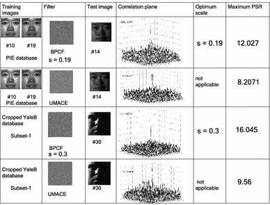
Improvement in PSR value for authentic persons (for both PIE and YaleB) under poor lighting condition is observed with BPCF comparing to UMACE filter
\(\mathrm {PSR}>10\) indicates authentic and \(\mathrm {PSR}<10\) indicates impostor.
Fig. 5 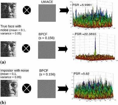
Correlation planes in response to noisy authentic image using different correlation filters. The point spread function of each filter is shown


References
Jeong, K., Liu, W., Han, S., Hasanbelliu, E., Principe, J.: The correntropy MACE filter. Pattern Recogn. 42(9), 871–885 (2009)
Yan, Y., Zhang, Y.: 1D correlation filter based class-dependence feature analysis forface recognition. Pattern Recogn. 41, 3834–3841 (2008)
Banerjee, P.K., Datta, A.K.: Generalized regression neural network trained preprocessing of frequency domain correlation filter for improved face recognition and its optical implementation. Opt. Laser Technol. 45, 217–227 (2013)
Banerjee, P.K., Datta, A.K.: A preferential digitaloptical correlator optimized by particle swarm technique for multi-class face recognition. Opt. Laser Technol. 50, 33–42 (2013)
Banerjee, P.K., Datta, A.K.: Class specific subspace dependent nonlinear correlation filtering for illumination tolerant face recognition. Pattern Recogn. Lett. 36, 177–185 (2014)
Levine, M., Yu, Y.: Face recognition subject to variations in facial expression, illumination and pose using correlation filters. Comput. Vis. Image Underst. 104(115), 1–15 (2006)
Lai, H., Ramanathan, V., Wechsler, H.: Reliable face recognition using adaptive and robust correlation filters. Comput. Vis. Image Underst. 111, 329–350 (2008)
Maddah, M., Mozaffari, S.: Face verification using local binary pattern-unconstrained minimum average correlation energy correlation filters. J. Opt. Soc. Am. A 29(8), 1717–1721 (2012)
Rodrguez, R., Mndez-Vzquez, H., Garca-Reyes, E.: Illumination invariant face recognition using quaternion-based correlation filters. J. Math. imaging Vis. 45(2), 164–643 (2013). doi:10.1007/s10851-012-0352-0
Rodriguez, A., Boddeti, V., Kumar, B., Mahalanobis, A.: Maximum margin correlation filter: A new approach for localization and classification. IEEE Trans. Image Process. 22(2), 631–643 (2013)
G. Heusch, F. Cardinaux, S. Marcel: Lighting Normalization Algorithms for Face Verification. Lighting normalization algorithms for face verification. Idiap-Com Idiap-Com-03-2005, IDIAP (2005)
Chen, W., Er, M., Wu, S.: Illumination compensation and normalization for robust face recognition using discrete cosine transform in logarithmic domain. IEEE Trans. Syst. Man Cybern. Part B 36, 458–466 (2006)
S. Du, R. Ward: Wavelet-Based illumination normalization for face recognition. In: Proceedings of the IEEE International Conference on Image Processing, pp. 954–957, (2005)
S.D. Wei, S.H. Lai: Robust face recognition under lighting variations. Proc. Intl. Conf. Pattern Recogn. 00(C), 354–357 (2004)
C.H.T. Yang, S.H. Lai, L.W. Chang: Robust face matching under different lighting conditions. In: ICME (2) (IEEE, 2002), pp. 149–152
Zhao, W., Chellappa, R.: Illumination-insensitive face recognition using symmetric shape-from-shading. Proc. CVPR00 1, 286–293 (2000)
Georghiades, A.S., Belhumeur, P.N., Kriegman, D.J.: From few to many: illumination cone models for face recognition under variable lighting and pose. IEEE Trans. Pattern Anal. Mach. Intell. 23, 643–660 (2001)
M. Savvides, B. Kumar, In: Proceedings of the IEEE Conference on Advanced Video and Signal Based Surveillance (AVSS 03) (2003)
M. Savvides, K. Venkataramani, B. Kumar: Incremental updating of advanced correlation filters for biometric authentication systems. In: Proc. of IEEE Int. Conf. on Multimedia and Expo, vol. III, p. 229 (2003)
Savvides, M., Kumar, B.: Illumination Normalization Using Logarithm Transforms for Face Authentication. Lecture Notes in Computer Science, Springer 2688, 549–556 (2003)
Banerjee, P.K., Datta, A.K.: Illumination and noise tolerant face recognition based on eigen-phase correlation filter modified by Mexican hat wavelet. J. Opt. 38(3), 160–168 (2009)
Mahalanobis, A., Kumar, B., Casassent, D.: Minimum average correlation energy filter. Appl. Opt. 26(17), 3633–3640 (1987)
Mahalanobis, A., Kumar, B., Song, S., Sims, S., Epperson, J.: Unconstrained correlation filter. Appl. Opt. 33, 3751–3759 (1994)
Kumar, B., Savvides, M., Xie, C., Venkataramani, K., Thornton, J., Mahalanobis, A.: Biometric verification with correlation filters. Appl. Opt. 43(2), 391–402 (2004)
Surez, D.A., Salazar, A.: Comparative study of pattern correlation using Mexican hat and Coiflet wavelet-based filtering. Opt. Commun. 282, 4203–4209 (2009)
Goyale, S., Nischal, N.K., Beri, V.K., Gupta, A.K.: Wavelet-modified maximum average correlation height filter for rotation invariance that uses chirp encoding in a hybrid digital-optical correlator. Appl. Opt. 45(20), 4850–4857 (2006)
Kumar, B.: Minimum variance synthetic discriminant functions. J. Opt. Soc. Am. A 3(10), 1579–1584 (1986)
B. Kumar, M. Alkanhal: Eigen-extended maximum average correlation height (EEMACH) filters for automatic target recognition. Proc. SPIE 4379, Automatic Target Recognition XI 4379, 424–431 (2001)
Lee, K., Ho, J., Kriegman, D.: Acquiring linear subspaces for face recognition under variable lighting. IEEE Trans. Pattern Anal. Mach. Intell. 27(5), 684–698 (2005)
Sim, T., Baker, S., Bsat, M.: The CMU pose illumination, and expression database. IEEE Trans. Pattern Anal. Mach. Intell. 25(12), 1615–1618 (2003)
M. Savvides, B. Kumar, P. Khosla: Corefaces- Robust Shift Invariant PCA based Correlation Filter for Illumination Tolerant Face Recognition. In: Proceedings of the 2004 IEEE Computer Society Conference on Computer Vision and Pattern Recognition (CVPR04) (2004)
Author information
Authors and Affiliations
Corresponding author
Rights and permissions
About this article

Cite this article
Banerjee, P.K., Datta, A.K. Band-pass correlation filter for illumination- and noise-tolerant face recognition. SIViP 11, 9–16 (2017). https://doi.org/10.1007/s11760-016-0882-9
Received:
Revised:
Accepted:
Published:
Issue Date:
DOI: https://doi.org/10.1007/s11760-016-0882-9