
Abstract
This paper derives the bounded real lemmas corresponding to L ∞ norm and H ∞ norm (L-BR and H-BR) of fractional order systems. The lemmas reduce the original computations of norms into linear matrix inequality (LMI) problems, which can be performed in a computationally efficient fashion. This convex relaxation is enlightened from the generalized Kalman-Yakubovich-Popov (KYP) lemma and brings no conservatism to the L-BR. Meanwhile, an H-BR is developed similarly but with some conservatism. However, it can test the system stability automatically in addition to the norm computation, which is of fundamental importance for system analysis. From this advantage, we further address the synthesis problem of H ∞ control for fractional order systems in the form of LMI. Three illustrative examples are given to show the effectiveness of our methods.
1 Introduction
Fractional order systems (FOSs) have attracted extensive attention during the past few years. Numerous investigations point out that fractional phenomena are encountered in many physics and engineering sciences, such as electromagnetics[1] and quantum mechanics[2].Moreover, with the theoretical development of fractional differential equations[3], fractional controllers have been proposed which possess more flexibilities and robustness, e.g., the PIλDu controller[4], the CRONE principle[5], and other variations[6]. Many fundamentals and applications of fractional order control systems can be found in [7] and the references therein.
Stability and norms are important system specifications which are also the research focus in the area of FOSs. Matignon[8] studied linear time invariant FOSs and laid the theoretical foundation of the stability analysis in 1998. Further, it was revealed that linear or nonlinear FOSs have more general stability type called Mittag-Leffler stability in contrast to the classical exponential stability[9]. Many linear matrix inequality (LMI) criteria are available for the stability and robustness of certain or uncertain FOSs[10–15]. On the other hand, it is well known that H2 and H∞ norms are significant quantities associated with control system performance such as robust stability, disturbance rejection and measurement noise attenuation. An analytical computation method for the H2 norm of FOSs was derived in [16]. Fadiga et al.[17, 18] proposed some LMI-based and Hamiltonian-matrix-based methods for the H∞ norm computation of FOSs. Similarly, a bounded real lemma for FOSs was derived in [19]. It is also interesting to mention some recent studies with respect to H∞ controls and approximations of FOSs[20–24].
Despite the plentiful achievements, there is room for further investigation. Firstly, the norm considered in [17–19] is actually the L∞ norm rather than H∞ norm, which will be explained and clarified in Section 2. Since the L∞ norm is irrelative to system stability, it is insufficient for analysis and synthesis of control systems. Secondly, the computation method in [18] and the bounded real lemma in [19] are conservative since the criteria are sufficient but not necessary. The conservatism will result in over estimation of the norm, i.e., only its upper bound is obtained. Sufficient and necessary conditions for the exact norm computation and controller synthesis are proposed respectively in [17, 20], whereas the conditions are in the form of nonlinear matrix inequalities. They cannot be directly solved by LMI technique or any other convex optimization. Tractable solutions of them require employing additional iteration algorithms which aggravate the computational burden. Thirdly, a bounded real lemma for the H∞ norm of FOSs should be able to test the system stability and compute the norm simultaneously, which is a more difficult task than the L∞ one. To the best of our knowledge, looking for such a kind of bounded real lemma for FOSs with both theoretical thoroughness and computational advantage still remains open.
Motivated by the discussions above, this paper derives the bounded real lemmas for FOSs. Novel results possessing computational advantage are obtained by employing the so-called generalized Kalman-Yakubovich-Popov (KYP) lemma to transform the problems into LMI formations that can be efficiently solved. Besides, the theoretical contributions of this work are as follows. Firstly, the bounded real lemma corresponding to L∞ norm (L-BR) of FOSs is derived without any conservatism. Secondly, the bounded real lemma corresponding to H∞ norm (H-BR) of FOSs is proposed that performs stability test and norm computation simultaneously. Thirdly, the synthesis problem of H∞controller for FOSs is addressed by applying the H-BR.
The rest of this paper is organized as follows. Section 2 provides some preliminaries for FOSs and the corresponding norms. In Section 3, the L-BR and H-BR are proposed. In Section 4, the synthesis problem of H∞ controller for FOSs is addressed. In Section 5, three illustrative examples are given. Finally, Section 6 concludes the paper.
Notations. For matrix X, the transpose and complex conjugate transpose are denoted by XT and X* Respectively. Sym(X) is short for X + X*, and σmax(X) represents the maximum singular value of X. Expression X > 0 (X < 0) indicates that X is positive (negative) definite. Symbols Cn×m and Rn×m stand for sets of n × m complex and real matrices, respectively. Symbol H n represents the set of n × n complex Hermitian matrices, and I n stands for an n × n unit matrix. The operator ⊗ is the Kronecker’s product. Finally, the real part of a complex number s is denoted by Re(s).
2 Preliminaries
Consider the following FOS
where α is the fractional commensurate order, x(t) ∈ Rn, u(t) ∈ Rm and y(t) ∈ Rp denote the pseudo state, control vector and output vector, respectively. The Caputo’s definition is adopted for fractional order derivative as
where k is a positive integer and k − 1 ≤ γ < k. If the FOS (1) is relaxed at t = 0, it can be equivalently represented by the transfer function matrix
To avoid conceptual confusion for the norms of FOSs, we introduce the following definitions which are consistent with the traditional ones as in [25].
-
Definition 1. The L∞ norm of G(s) is defined as
$${\left\Vert {G(s)} \right\Vert _{{L_\infty}}} \buildrel \Delta \over = \mathop {\sup}\limits_{\omega \in {\rm{R}}} {\sigma _{\max}}(G({\rm{j}}\omega)).$$(4) -
Definition 2. The H∞ norm of G(s) is defined as
$${\left\Vert {G(s)} \right\Vert _{{H_\infty}}} \buildrel \Delta \over = \mathop {\sup}\limits_{{\rm{Re(s)}} \geq {\rm{0}}} {\sigma _{\max}}(G(s)).$$(5)It should be noted that the norm concerned in [17–19] is in accordance with (4). Therefore, those previous results actually correspond to the L∞ norm rather than the H∞ norm.
Several useful lemmas are given as follows.
-
Lemma 1[26]. Let matrices A ∈ Rn×n, B ∈ Rn×m, Θ ∈ H(n+m), Φ ∈ H2 and Ψ ∈ H2. Set Λ is defined as
$$\Lambda (\Phi ,\Psi) \buildrel \Delta \over = \left\{{\lambda \in {\bf{C}}\vert {{\left[ {\matrix{\lambda \cr1 \cr}} \right]}^{\ast}}\;\Phi \left[ {\matrix{\lambda \cr1 \cr}} \right] = 0,\;{{\left[ {\matrix{\lambda \cr1 \cr}} \right]}^{\ast}}\;\Psi \left[ {\matrix{\lambda \cr1 \cr}} \right] \geq 0} \right\}.$$(6)Consider the following two statements:
-
1)
For H (λ) ≜ (λI n − A)−1B, there holds
$${\left[ {\matrix{{H(\lambda)} \cr{{I_m}} \cr}} \right]^{\ast}}\Theta \left[ {\matrix{{H(\lambda)} \cr{{I_m}} \cr}} \right] < 0,\quad \forall \lambda \in \Lambda .$$(7) -
2)
There exist P, Q ∈ H n and Q > 0 such that
 ((8))
((8))Then “2) ⇒ 1)” always holds. Moreover, if Λ represents a curve in the complex plane, there holds “2) ⇔ 1)”.
-
1)
-
Lemma 2. Let set Λ(Φ, Ψ) in Lemma 1 be replaced by Υ(Φ, Ψ), which is defined as
$$\Upsilon (\Phi ,\Psi) \buildrel \Delta \over = \left\{{\lambda \in {\bf{C}}\vert {{\left[ {\matrix{\lambda \cr1 \cr}} \right]}^{\ast}}\Phi \left[ {\matrix{\lambda \cr1 \cr}} \right] \geq 0,\;{{\left[ {\matrix{\lambda \cr1 \cr}} \right]}^{\ast}}\;\Psi \left[ {\matrix{\lambda \cr1 \cr}} \right] \geq 0} \right\}.$$(9)Then, LMI of (7) holds for ∀λ ∈ Υ if there exist matrices P > 0 and Q > 0 such that LMI of (8) holds.
-
Proof. Please see the Appendix. □
-
Lemma 3[8]. The fractional order system G(s)in (3) is stable if and only if \({\left\Vert {G(s)} \right\Vert _{{H_\infty}}}\), is bounded.
-
Lemma 4[11]. The fractional order system Dαx(t) = Ax(t) is stable if and only if either one of the following two statements holds:
-
1)
\(\vert \arg ({\rm{spec}}(A))\vert > {\textstyle{\pi \over 2}}\alpha\), where spec(A) is the spectrum (set of eigenvalues) of A.
-
2)
Let \(\theta \buildrel \Delta \over = {\textstyle{\pi \over 2}}(1 - \alpha)\). For the case 1 ≤ α < 2, there exists P > 0 such that Sym(ejθ i) < 0. For the case 0 < a < 1, there exist P > 0 and Q > 0 such that Sym(ejθ AP + e−jθ AQ) < 0.
-
1)
-
Lemma 5. For a fractional order system G(s), there holds
$${\left\Vert {G(s)} \right\Vert _{{{\cal L}_\infty}}} = \mathop {\sup}\limits_{\omega \geq 0} {\sigma _{\max}}(G(j\omega)).$$ -
Proof. Please see the Appendix. □
-
Remark 1. Lemma 1 is the well-known generalized KYP lemma which can be regarded as a kind of convex relaxation. The relaxed LMI condition is always sufficient for the corresponding counterpart. This is also true for Lemma 2 in the same way. These two lemmas are key tools for relaxations of the original norm computations. Lemma 3 reveals that H∞ norm is capable of ascertaining the stability of FOS, which is the theoretical foundation of H∞ control strategy for FOS. Lemma 5 indicates that one needs only to consider the positive half imaginary axis for the L∞ norm computation, which will simplify its convex relaxation as well.

3 Bounded real lemmas for FOS
Now we are ready to present the L-BR and H-BR for FOSs.
-
Theorem 1 (L-BR). Consider an FOS with its transfer function G(s)in (3). Then \({\left\Vert {G(s)} \right\Vert _{{L_\infty}}} < \gamma\) if and only if there exist P, Q ∈ H n and Q > 0 such that
 (10)
(10)where \(X \buildrel \Delta \over = {{\rm{e}}^{{\rm{j}}\theta}}P(1 - \alpha)Q\) and \(\theta {\text{ }} \triangleq \frac{\pi } {2}(1 - \alpha ) \).
-
Proof. Let \(\lambda (\omega) \buildrel \Delta \over = {{\rm{e}}^{- {\rm{j}}{\textstyle{\pi \over 2}}\alpha}}{\omega ^\alpha}\), we have \({({\rm{j}}\omega)^\alpha} = {{\rm{e}}^{{\rm{j}}{\textstyle{\pi \over 2}}\alpha}}{\omega ^\alpha} = \lambda \ast (\omega),\quad \forall \omega \geq 0\). Then it follows from Lemma 5 that \({\left\Vert {G(s)} \right\Vert _{{L_\infty}}} = {\sup _{\omega \geq 0}}{\sigma _{\max}}(C{(\lambda \ast (\omega){I_n} - A)^{- 1}}B + D)\). Meanwhile, when ω ranges from 0 to +∞, λ(ω) varies along a ray in the complex plane. This ray can be represented by Λ(Φ, Ψ) in (6) with

By some basic matrix calculations, we have
 ((11))
where H(λ) ≜ (λI n − AT)−1CT and

According to Lemma 1, the last part of (11) is also equivalent to the statement that ∃P, Q ∈ H n and Q > 0 such that the following LMI holds
 ((12))
The above LMI can be further simplified as
 ((13))
where X = ejθP + (1 − α)Q. Rescaling X and utilizing the Schur complement theorem, we obtain that LMI (13) is equivalent to LMI (10). □
-
Remark 2. Theorem 1 provides a sufficient and necessary LMI condition of the L∞ norm, which can be efficiently solved and is free of any conservatism. Therefore, this L-BR is superior to the existing results in [17–19].
-
Theorem 2 (H-BR). Consider the FOS with its transfer function G(s)in(3). Then \({\left\Vert {G(s)} \right\Vert _{{H_\infty}}} < \gamma\) if there exist P > 0 and Q > 0 such that the following LMI holds
 ((14))
where

Moreover, in the case 1 ≤ α ≤ 2, the LMI condition (14) is also necessary.
-
Proof. Basically, the proof follows the procedure that 1) specifying a proper region corresponding to H∞ norm, 2) representing the region by LMI descriptions in (9), 3) relaxing the norm condition into LMI by using Lemma 2.
Firstly, it is a fact that for any subregion Ω in the complex plane satisfying \(\Omega \cup \bar \Omega = \{{s^\alpha}\vert s \in C,{\rm{Re}}(s) \geq 0\}\), where \(\bar \Omega\) is the symmetrical region of Ω with respect to the real axis, there must hold \({\left\Vert {G(s)} \right\Vert _{{H_\infty}}} = {\sup _{{\rm{Re}}(s) \geq 0}}{\sigma _{\max}}(G(s)) = {\sup _{s \in \Omega}}\;{\sigma _{\max}}(G(s))\). This just follows from the maximum modulus principle and the complex conjugate symmetry of G(s).
Secondly, it is easy to verify that \(\{{s^\alpha}\vert s \in {\bf{C}},{\rm{Re}}(s) \geq 0\} = \Upsilon \cup \bar \Upsilon\), where Υ is defined in (9) with its detailed data as

Thirdly, from the previous two steps, the sufficiency of LMI (14) can be proved by using Lemma 2 in a similar way to Theorem 1. Thus, it is omitted here. Then the remaining proof is the necessity of LMI (14) for the case 1 ≤ α ≤ 2. Suppose that 1 ≤ α < 2 and \({\left\Vert {G(s)} \right\Vert _{{{\cal H}_\infty}}} < \gamma\). Noting that the curve
 in (6) belongs to {sα|s ∈ C, Re(s) ≥ 0}, we have \({\sup _{s \in {\Lambda _1}}}{\sigma _{\max}}(G(s)) \leq {\left\Vert {G(s)} \right\Vert _{{{\cal H}_\infty}}} < \gamma\). It implies that according to Lemma 1, there exists P ∈ H
n
such that
in (6) belongs to {sα|s ∈ C, Re(s) ≥ 0}, we have \({\sup _{s \in {\Lambda _1}}}{\sigma _{\max}}(G(s)) \leq {\left\Vert {G(s)} \right\Vert _{{{\cal H}_\infty}}} < \gamma\). It implies that according to Lemma 1, there exists P ∈ H
n
such that  ((15))
Further, it follows from the Schur complement theorem that LMI (15) is equivalent to LMI (14) with X =ejθ P. Then the only remaining is to prove that matrix P is positive definite. To prove this, we notice that LMI (14) implies Sym(AX) < 0. Thus, there exists M > 0 such that ejθ AP + P(ejθA)* = −M. On the other hand, \({\left\Vert {G(s)} \right\Vert _{{{\cal H}_\infty}}} < \gamma\) implies that G(s) is stable. Then according to Lemma 4, we have \(\arg ({\rm{spec}}(A)) > {\textstyle{\pi \over 2}}\alpha\), i.e., all the eigenvalues of ejθ A are in the left half complex plane. Therefore, we have \(P = \int_0^{+ \infty} {{{\rm{e}}^{{{\rm{e}}^{{\rm{j}}\theta}}At}}} M{{\rm{e}}^{({{\rm{e}}^{{\rm{j}}\theta}}A)\ast t}}\;{\rm{d}}t > 0\) □
-
Remark 3. In thecaseof 1 ≤ α < 2, an exactly same result was obtained in [21].
-
Remark 4. The feasibility of LMI (14) implies Sym(AX) < 0, which is exactly the necessary and sufficient LMI condition for the stability of FOSs according to Lemma 4.


 in (
in (
4 H∞ controller synthesis for FOS
As mentioned in the previous section, the H-BR can ascertain the system stability. Thus, it can be applied to the controller synthesis. Since the results involve complex matrices in LMI (14) whereas the control gain must be real, a further treatment is proposed as follows.
Consider the following FOS
where x(t) ∈ Rn and u(t) ∈ Rm, z(t) ∈ Rp and w ∈ Rq are the regulated output and the exogenous input, respectively. With static state feedback u(t)= Kx(t), the closed loop system has the transfer function from w to z in the following
-
Theorem 3 controller synthesis). Consider the FOS (16) with transfer function G wz (s) in (17), and the following LMI
 ((18))
Let \(\theta = {\pi \over 2}(1 - \alpha)\), then there holds \({\left\Vert {{G_{wz}}(s)} \right\Vert _{{H_\infty}}} < \gamma\) if

Moreover, the static state feedback gain matrix can be obtained by K = YX−1.
-
Proof. Thecase1 ≤ α < 2 can be straightforwardly proved by utilizing Theorem 2 and is omitted here.
For the case 0 < α < 1, let \(\tilde P \buildrel \Delta \over = P + {\rm{j}}Q\) and \(\tilde Q \buildrel \Delta \over = P - {\rm{j}}Q\). Then we have \(\tilde P > 0\) and \({\tilde Q^{\rm{T}}} > 0\) (the transposition does not change the eigenvalues of a matrix). It follows from some basic calculation that \(X = \cos (\theta)P + \sin (\theta)Q = {{\rm{e}}^{{\rm{j}}\theta}}\tilde P + {{\rm{e}}^{- {\rm{j}}\theta}}\tilde Q\). According to Theorem 2, the feasibility of LMI (18) implies \({\left\Vert {{G_{wz}}(s)} \right\Vert _{{H_\infty}}} < \gamma\).
Finally, in order to illustrate that the derived gain matrix K is real and available, we first notice that matrix X is real since P and Q are real matrices. Moreover, X is non-singular because \(\tilde P,\tilde Q > 0\) implies \({v^{\rm{T}}}Xv = {{\rm{e}}^{{\rm{j}}\theta}}({v^{\rm{T}}}\tilde Pv) + {{\rm{e}}^{- {\rm{j}}\theta}}({v^{\rm{T}}}\tilde Qv) = \cos \theta (({v^{\rm{T}}}\tilde Pv) + ({v^{\rm{T}}}\tilde Qv)) > 0,\forall v \in {{\bf{R}}^n}\). Therefore, a real static state feedback gain matrix is available by K = YX−1. □
-
Remark 5. The decision matrices in Theorem 3 are cast as real matrices in comparison with Theorem 2. This will bring some conservatism of the controller.
5 Numerical examples
-
Example 1. Consider the following FOS
$$G(s) = {{{s^{0.5}} + 1} \over {s + 2{s^{0.5}} + 5}}.$$The pseudo state space realization is

Using the L-BR and H-BR, we obtain \({\left\Vert {G(s)} \right\Vert _{{H_\infty}}} < 0.2817\) and \({\left\Vert {G(s)} \right\Vert _{{L_\infty}}} < 0.2774\). It follows from \({\left\Vert {G(s)} \right\Vert _{{H_\infty}}} < + \infty\) that G(s) is stable. Therefore, we have
$${\left\Vert {G(s)} \right\Vert _{{H_\infty}}} = {\left\Vert {G(s)} \right\Vert _{{L_\infty}}} = 0.2774.$$To illustrate the correctness, we consider
$$G({\rm{j}}\omega) = {{{{({\rm{j}}\omega)}^{0.5}} + 1} \over {{{({{({\rm{j}}\omega)}^{0.5}} + 1)}^2}4}}.$$For its L∞, norm, we need only to consider the ω ≥ 0 part. Then, it follows from the bijection x = ωα:[0, + ∞) → [0, +∞) that \(G({\rm{j}}\omega) = \tilde G(x)\), where
$$\tilde G(x) = {{{{\rm{e}}^{{\rm{j}}{\textstyle{\pi \over 4}}}}x + 1} \over {{{({{\rm{e}}^{{\rm{j}}{\textstyle{\pi \over 4}}}}x + 1)}^2} + 4}}.$$Then, it can be obtained that \({\left\Vert {G(s)} \right\Vert _{{L_\infty}}} = {\max _{x \geq 0}}\vert G(x)\vert = 0.2774\), as shown in the image of |G(x)| in Fig. 1.
-
Remark 6. According to Fig. 1, the maximum peak point of \(\vert \tilde G(x)\vert\) for −∞ < x < +∞ is at x = −2.282 and \({\max _{- \infty < x < + \infty}}\vert \tilde G(x)\vert = 0.6495\). However, it is an upper bound rather than the exact value of the L∞ norm of G(s). Therefore, constraint x ≥ 0 is necessary. In fact, it reveals that the matrix item Q in X = ejθ P+(1 − α)Q of the L-BR is necessary and eliminates the conservatism.
-
Example 2. Consider the following FOS
$$G(s) = {{{s^{1.5}} + 1} \over {{s^3} + 2{s^{1.5}} + 5}}.$$The pseudo state space realization is

Using the L-BR and H-BR, we obtain \({\left\Vert {G(s)} \right\Vert _{{L_\infty}}} = 0.6495\) and find that the LMI condition of H-BR is infeasible, i.e., \({\left\Vert {G(s)} \right\Vert _{{H_\infty}}} = + \infty\). In fact, this system is not stable because the eigenvalues of the system matrix are − 1 ± 2j, which satisfy \(\vert \arg (- 1 \pm 2{\rm{j}})\vert < 1.5 \times {\textstyle{\pi \over 2}}\). It verifies that the H-BR tests the system stability automatically whereas the L-BR does not.
-
Example 3. Consider the system

The open loop transfer function, i.e., with u =0, is
$${G_{owz}}(s) = {{{s^{0.5}} + 0.2} \over {s + 0.4{s^{0.5}} + 0.2}}.$$For a desired weighting function \(W(s) = {1 \over {s + 1}}\), an augmented model of W(s)G owz (s) can be formulated as
$$\left\{{\matrix{{{D^{0.5}}\tilde x(t) = A\tilde x(t) + Bu(t) + {B_1}w} \hfill \cr{z(t) = C\tilde x(t)} \hfill \cr}} \right.$$where
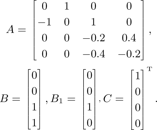
It can be obtained that \({\left\Vert {W(s){G_{owz}}(s)} \right\Vert _{{H_\infty}}} = 1.382\). For the requirement that the weighted H∞ norm of the closed loop system be less than γ = 1, by using LMI method given in Theorem 3 we obtain the control gain matrix K =[−4.977, −2.374, 0.0157, −0.359]. Then, the transfer function of the closed loop system is
$${G_{cwz}}(s) = {{{s^{0.5}} + 0.559} \over {{s^2} + 0.7431{s^{1.5}} + 3.492s + 7.145{s^{0.5}} + 3.105}}$$with the weighted norm \({\left\Vert {W(s){G_{cwz}}(s)} \right\Vert _{{H_\infty}}} = 0.18\). The improvement for H∞ performance of the control system is also shown by the Bode diagram of W(s)G owz (s) and W(s)G cwz (s) in Fig. 2.


Modulus of transformed function \(\tilde G(x)\) in Example 1, where the maximal value of the x ≥ 0 part corresponds to the norm of the original FOS G(s)

Bode diagrams of the weighted open and closed loop systems in Example 3, i.e., W(s)G owz (s) and W(s)G cwz (s), respectively
6 Conclusions
This paper has derived the bounded real lemmas corresponding to L∞ norm and H∞ norm of fractional order systems. Both of them convert the original computations of norms into LMI problems, which can be efficiently solved. The L-BR has no conservatism and yields the exact value of L∞ norm. The H-BR is conservative for H∞ norm computation but can test the stability of FOSs automatically. The synthesis problem of H∞ controller for FOSs has been solved based on the proposed H-BR. Future research subjects will include how to reduce or overcome the existing conservatism in the H∞ norm computation and the H∞ controller synthesis.
References
T. Machado, I. S. Jesus, A. Galhano, J. B. Cunha. Fractional order electromagnetics. Signal Processing, vol. 86, no. 10, pp. 2637–2644, 2006.
T. N. Laskin. Fractional quantum mechanics and Levy path integrals. Physics Letters, vol. 268, no. 4, pp. 298–305, 2000.
I. Podlubny. Fractional Differential Equations, San Diego, USA: Academic Press, 1999.
I. Podlubny. Fractional-order systems and PI λ D μ controllers. IEEE Transactions on Automatic Control, vol. 44, no. 1, pp. 208–214, 1999.
A. Oustaloup, X. Moreau, M. Nouillant. The CRONE suspension. Control Engineering Practice, vol. 4, no. 8, pp. 1101–1108, 1996.
S. Arunsawatwong, Q. Nguyen. Design of retarded fractional delay differential systems using the method of inequalities. International Journal of Automation and Computing, vol. 6, no. 1, pp. 22–28, 2009.
C.M. Monje, Y. Q. Chen, B.M. Vinagre, D. Xue, V. Feliu. Fractional Order Systems and Controls: Fundamentals and Applications, London, England: Springer-Verlag, 2010.
D. Matignon. Stability properties for generalized fractional differential systems. ESAIM: Proceedings, vol. 5, pp. 145–158, 1998.
Y. Li, Y. Q. Chen, I. Podlubny. Mittag-Leffler stability of fractional order nonlinear dynamic systems. Automatica, vol. 45, no. 8, pp. 1965–1969, 2009.
Z. Liao, C. Peng, W. Li, Y. Wang. Robust stability analysis for a class of fractional order systems with uncertain parameters. Journal of the Franklin Institute, vol. 348, no. 6, pp. 1101–1113, 2011.
J. Sabatier, M. Moze, C. Farges. LMI stability conditions for fractional order systems. Computers and Mathematics with Applications, vol. 59, no. 5, pp. 1594–1609, 2010.
S. Liang, C. Peng, Y. Wang. Improved linear matrix inequalities stability criteria for fractional order systems and robust stabilization synthesis: The 0 < α < 1 case. Control Theory and Applications, vol. 30, no. 4, pp. 531–535, 2013.
Y. Wang, S. Liang. Two-DOF lifted LMI conditions for robust D-stability of polynomial matrix polytopes. International Journal of Control, Automation and Systems, vol. 11, no. 3, pp. 636–642, 2013.
Y. H. Lan, W. J. Zhou, Y. P. Luo. Non-fragile observer design for fractional-order one-sided Lipschitz nonlinear systems. International Journal of Automation and Computing, vol. 10, no. 4, pp. 296–302, 2013.
J. G. Lu, Y. Q. Chen. Robust stability and stabilization of fractional-order interval systems with the fractional order α: The 0 < α < 1 case. IEEE Transactions on Automatic Control, vol. 55, no. 1, pp. 152–158, 2010.
R. Malti, M. Aoun, F. Levron, A. Oustaloup. Analytical computation of the H 2 norm of fractional commensurate transfer functions. Automatica, vol. 47, no. 11, pp. 2425–2432, 2011.
L. Fadiga, C. Farges, J. Sabatier, M. Moze. On computation of H ∞ norm for commensurate fractional order systems. In Proceedings of the 50th IEEE Conference on Decision and Control and European Control Conference, IEEE, Orlando, FL, USA, pp. 8231–8236, 2011.
J. Sabatier, M. Moze, A. Oustaloup. On fractional systems H ∞ norm computation. In Proceedings of the 44th IEEE Conference on Decision and Control and European Control Conference, IEEE, Seville, Spain, pp. 5758–5763, 2005.
M. Moze, J. Sabatier, A. Oustaloup. On bounded real lemma for fractional systems. In Proceedings of the 17th IFAC World Congress, IFAC, COEX, Korea, pp. 15267–15272, 2008.
S. Liang, C. Peng, Z. Liao, Y. Wang. State space approximation for general fractional order dynamic systems. International Journal of Systems Science, vol. 45, no. 10, pp. 2203–2212, 2014.
L. Fadiga, J. Sabatier, C. Farges. H ∞ state feedback control of commensurate fractional order systems. In Proceedings of IFAC Workshop on Fractional Differentiation and Its Applications, IFAC, Grenoble, France, vol. 6, pp. 54–59, 2013.
J. Shen, J. Lam. State feedback H ∞ control of commensurate fractional-order systems. International Journal of Systems Science, vol. 45, no. 3, pp. 363–372, 2014.
J. Shen, J. Lam. H ∞ model reduction for positive fractional order systems. Asian Journal of Control, vol. 16, no. 2, pp. 441–450, 2014.
L. Fadiga, C. Farges, J. Sabatier, K. Santugini. H ∞ output feedback control of commensurate fractional order systems. In Proceedings of the European Control Conference, IEEE, Zurich, Switzerland, pp. 4538–4543, 2013.
M. Green, D. J. N. Limebeer. Linear Robust Control, NJ, USA: Upper Saddle River, Prentice-Hall, Inc., 1995.
T. Iwasaki, S. Hara. Generalized KYP lemma: Unified frequency domain inequalities with design applications. IEEE Transactions on Automatic Control, vol. 50, no. 1, pp. 41–59, 2005.
Acknowledgements
The authors would like to thank the anonymous reviewers for their insightful comments which improved the contents of this paper. The authors would also like to thank Dr. Cheng Peng and Dr. Zeng Liao for their suggestive help on this research, and Dr. Xi Zhou for pointing out some mistakes in the previous version of this paper.
Author information
Authors and Affiliations
Corresponding author
Additional information
This work was supported by National Natural Science Foundation of China (Nos. 61004017 and 60974103).
Recommended by Associate Editor James Whidborne
Appendix
Appendix
-
Proof for Lemma 2. Suppose that there exist matrices P, Q > 0 such that LMI (8) holds. Then, it follows from some matrix calculations that
 ((19))
Noting that for any γ ∈ Υ, there hold \({\left[ {\matrix{\lambda \cr 1 \cr}} \right]^{\ast}}\Phi \left[ {\matrix{\lambda \cr 1 \cr}} \right] \geq 0\) and \({\left[ {\matrix{\lambda \cr 1 \cr}} \right]^{\ast}}\Psi \left[ {\matrix{\lambda \cr 1 \cr}} \right] \geq 0\). In addition, since P, Q > 0, we also have H*(λ)PH(λ) > 0 and H*(λ) PH(λ) > 0. Therefore, it follows from these inequalities together with (19) that LMI (7) holds for ∇λ ∈ Υ. □
-
Proof for Lemma 5. Noting that the conjugate transpose does not change the eigenvalues of any matrix, we have σmax(G(s)) = σmax(G*(s)) for any s ∈ C. Meanwhile, since G(s) is the matrix transfer function with real coefficients, there holds G*(s) = G(s*). Therefore, we have \(\sup {\sigma _{\max}}(G({\rm{j}}\theta)) = \mathop {\sup}\limits_{\omega \geq 0} {\sigma _{\max}}(G(- {\rm{j}}\omega)) = \mathop {\sup}\limits_{\omega \leq 0} {\sigma _{\max}}(G({\rm{j}}\omega))\). □

Rights and permissions
About this article

Cite this article
Liang, S., Wei, YH., Pan, JW. et al. Bounded real lemmas for fractional order systems. Int. J. Autom. Comput. 12, 192–198 (2015). https://doi.org/10.1007/s11633-014-0868-4
Received:
Accepted:
Published:
Issue Date:
DOI: https://doi.org/10.1007/s11633-014-0868-4