
Abstract
Purpose
An open-source software system for planning magnetic resonance (MR)-guided laser-induced thermal therapy (MRgLITT) in brain is presented. The system was designed to provide a streamlined and operator-friendly graphical user interface (GUI) for simulating and visualizing potential outcomes of various treatment scenarios to aid in decisions on treatment approach or feasibility.
Methods
A portable software module was developed on the 3D Slicer platform, an open-source medical imaging and visualization framework. The module introduces an interactive GUI for investigating different laser positions and power settings as well as the influence of patient-specific tissue properties for quickly creating and evaluating custom treatment options. It also provides a common treatment planning interface for use by both open-source and commercial finite element solvers. In this study, an open-source finite element solver for Pennes’ bioheat equation is interfaced to the module to provide rapid 3D estimates of the steady-state temperature distribution and potential tissue damage in the presence of patient-specific tissue boundary conditions identified on segmented MR images.
Results
The total time to initialize and simulate an MRgLITT procedure using the GUI was \(<\)5 min. Each independent simulation took \(<\)30 s, including the time to visualize the results fused with the planning MRI. For demonstration purposes, a simulated steady-state isotherm contour \((57\,^{\circ }\hbox {C})\) was correlated with MR temperature imaging (N = 5). The mean Hausdorff distance between simulated and actual contours was 2.0 mm \((\sigma \,=\,0.4\,\hbox {mm})\), whereas the mean Dice similarity coefficient was 0.93 \((\sigma =0.026)\).
Conclusions
We have designed, implemented, and conducted initial feasibility evaluations of a software tool for intuitive and rapid planning of MRgLITT in brain. The retrospective in vivo dataset presented herein illustrates the feasibility and potential of incorporating fast, image-based bioheat predictions into an interactive virtual planning environment for such procedures.
Introduction
Magnetic resonance (MR)-guided laser-induced thermal therapy (MRgLITT) is an emerging minimally invasive approach for ablating targeted volumes of tissue in the brain. In a manner congruent with image-guided biopsy, laser applicators are stereotactically navigated under MR guidance to rapidly deliver heat to the target tissue [1]. MR temperature imaging (MRTI) [2, 3] can be used during delivery of therapy to quantitatively monitor the temperature changes in the volume of interest to estimate the extent of ablation using biological models of damage [4–6]. The primary mechanism of tissue destruction is thermal coagulation leading to thermal necrosis (i.e., death of cells) over the next 24–72 h [7]. This is a highly localized treatment, and unlike the radiation therapy, there are no known associated toxicities (e.g., ionizing radiation) that limit the multiple treatments, making the procedure repeatable up to the tolerance of the patient. Thermal therapy can also be applied in a manner complementary to the conventional approaches and can be used to treat additional focal lesions outside the range of conventional therapy or be used synergistically with local drug delivery [8, 9].
Magnetic resonance (MR)-guided laser-induced thermal therapy (MRgLITT) has been a viable therapeutic option for amenable primary, recurrent, and metastatic intracerebral lesions [10–12] and is being investigated for treating neurological diseases, such as epilepsy [13], and Tourette’s syndrome [14]. Currently, MRgLITT systems for closed-loop MR guidance in the brain are available commercially [11, 15–19]. In addition to providing the ability to monitor critical structures and lesion borders, such software uses the MRTI feedback to monitor the temperature near the applicator surface so that excessive temperatures leading to vaporization and charring do not occur. This provides another essential level of safety to the ablation procedure [19, 20]. However, because the procedure is somewhat invasive and requires stereotaxy to guide applicator placement directly into the tissue through the skull, preoperative planning is a critical component. A common approach is (1) to use a geometrical primitive cylindrical representation of the maximal thermal kill zone overlaid onto the 3D MRI for planning (e.g., contrast-enhanced T1-weighted MR gradient echo images), then (2) to identify a trajectory to the target tissue that avoids critical structures, and finally (3) to put the fiber in a position to deliver therapy as conformal as possible to the target area while avoiding irradiation of nontargeted tissue. However, estimating the potential extent of damage is a challenge if trajectories are oblique with respect to the anatomy, irregularly shaped lesions are targeted, or multiple applicators are employed. Additionally, nearby convective sources of heat transfer, e.g., ventricles, vessels, interfaces, etc., can lead to unexpectedly asymmetric temperature distributions, which deviate from planned treatment of volume.
In order to help maintain the efficacy of MRgLITT procedures under such complex conditions, and begin to fairly evaluate this technology with respect to existing therapeutic options, there is a critical need for patient-specific 3D treatment planning technology. Planning can aid in providing a more optimal initial placement of the applicator for therapy by letting the user to simulate treatment prospectively and visualizing results against the target volume and critical structures [21]. This can help streamline surgical planning and workflow and minimize the likelihood of positioning fibers in a manner inconsistent with therapeutic goals, avoiding the need to reposition/replace applicators or schedule a second treatment. To this end, we introduce an open-source 3D simulation-driven software system for planning MRgLITT in brain. Its graphical user interface (GUI) can facilitate the assessment of different treatment scenarios based on virtual adjustment of laser applicator(s) position/power relative to 3D anatomy and patient-specific bioheat parameters. The software may communicate with a variety of finite element, finite difference, and statistical modeling solution [22–24] techniques for the bioheat transfer equation through the designed interface. In this study, the software was interfaced with a steady-state bioheat solver to simulate different treatment approaches. The results were evaluated retrospectively using data from MRgLITT procedures in patients (N = 5).
Methodology
In this work, a loadable 3D Slicer module was developed as the core component of our software system to provide the neurosurgeon with an interactive GUI to plan the MRgLITT procedure using T1-weighted, T2-weighted, or Flair MRI. The module was named as LITTPlan, and its source code is freely available at the following github repository: https://github.com/ImageGuidedTherapyLab/LITTPlan. More specifically, LITTPlan module is designed to the following:
-
Assist neurosurgeons in navigating all identified critical structure volumes;
-
Visualize simulated heating at the final location of each applicator placement, with respect to adjoining critical structures and heat sinks;
-
Provide greater autonomous regulation and conformal delivery of energy.
-
Visually assess multiple structures in multiple planes to take full advantage of the entirety of digital information returned by the imaging guidance.
-
Provide the neurosurgeon with an intuitive, comprehensive, and dynamic perception of the target region.
A (conceptual) system to accommodate LITTPlan module consists of four main components as shown in Fig. 1. In such a system, multi-faceted intersystem communication can be facilitated via OpenIGTLink, which is an extensible digital messaging library with well-defined protocols for data exchange on local network [25]. OpenIGTLink can provide a standardized mechanism for real-time data flow between different hardware and software components of such systems. Tokuda et al., reported that it can perform data transfer up to 1,024 fps with latency in the order of sub-milliseconds [25], which is sufficient for on-the-fly data transfer in an environment as proposed herein. The operator/surgeon can use 3D Slicer in order to manage image acquisitions, necessary visual processing, and simulate laser application in different scenarios to implement a final strategic treatment plan. Potentially computationally intensive tasks of the solution to the bioheat transfer equation are implemented to run on the computational core and are expected to be responsive to the highly demanding interactive virtual planning environment. Please note that, currently the LITTPlan module communicates with the adapted bioheat transfer solver via an input text file, which includes all the patient-specific laser and treatment parameters.

An overview of the developed LITTPlan module within the MRgLITT workflow is shown. LITTPlan module was built on two correlated tasks, i.e., “Imaging” and “Planning.” T1-weighted contrast-enhanced, T2, and Flair images are used for delineating the target and surrounding critical tissues. In the planning phase, the label maps are created by segmentation and visualized on the GUI. Then, neurosurgeon can set the ablation parameters in addition to locating the applicator and call the finite element solver which in turn gives the calculated isotherm simulation model in near-real-time
Slicer
3D Slicer (or just Slicer) is an open-source, multi-platform (i.e., can work on Windows, Linux, and Mac OS) modular software system for performing highly demanding image analysis, processing, registration, and visualizations tasks [26, 27]. It has been developed by NIH support and used in more than 100 research projects so far [28, 29]. As one of the prominent examples of those projects, Pinter et al. introduced a comprehensive radiation therapy (RT) toolkit for Slicer. This extension allows loading, visualizing, and evaluating complex RT treatment plans on Slicer‘s intuitive GUI [28]. Moreover, Fedorov et al. [30] demonstrated the high potential of Slicer in quantitative image analysis for personalized treatment approaches by means of analyzing multiple use cases taken from the institutions participating in the Quantitative Image Network (QIN) initiative of National Cancer Institute. Slicer offers extensive functionality for overcoming the challenges of developing real-time image guidance research software of MRgLITT, such as visualization and segmentation of anatomical images, 3D registration (rigid, affine, and deformable), image-surface fusion, etc. It can read/write DICOM images, create,
and render volumes and polygonal meshes as well as allowing tool tracking and real-time acquisitions for image-guided interventions. Slicer allows customization and extension in the form of loadable modules. Its GUI-based interactive console allows performing calculations and processes that are highly demanding. Loadable modules can be developed using Python or C++. As shown in Fig. 2, Slicer is based on four layers of software abstraction over the computer hardware. Slicer’s core and custom modules are the main components for facilitating operational tasks such as image loading, processing, registration, transformations, etc., using the open-source programming libraries at one lower level such as Visualization Toolkit (VTK), Insight Segmentation, and Registration Toolkit (ITK) and a cross-platform application platform called QT. VTK is a freely available object-oriented software library for 3D virtual modeling and computer graphics, which is composed of C++ classes and supports a wide range of algorithms and modeling techniques. ITK is also an open-source development framework that provides an extensive set of functionality for image processing. Slicer extends those provided functionalities with the custom C++ modules specifically designed for medical imaging based applications [26, 30]. 3D Slicer version 4.2.2-1 (revision 21513) was used in this study and can be downloaded freely from the following website: http://www.slicer.org/slicerWiki/index.php/Slicer4.

OpenGL pipeline works at the lowest-level software layer for core visualization, while VTK, ITK, QT etc., libraries are included for providing higher-level programmable functionality such as 3D visualization, image processing, and registration. LITTPlan can incorporate with other modules as well as exchanging information with the Core
LITTPlan GUI
LITTPlan GUI has five expandable tab pages, namely: (1) Main, (2) Tissue Parameters, (3) Transformation, (4) Nodes, and (5) Advanced, as shown in Figs. 3 and 4. The “Main” tab provides the minimal functionality needed for planning the treatment. Tissue parameters, i.e., thermal conductivity, tissue perfusion, optical absorption, scattering, and anisotropy, on their corresponding tab, were set to the literature values for each tissue type by default [31, 32] (as listed Table 1). “Transformation” and “Nodes” tabs give the option of rotating and translating the models and the loaded images, whereas “Advanced” tab is used to adjust input/output file names and labelmap color codes. Prior to planning/simulating a treatment, different tissues in the target region (e.g., gray/white matter, edema, CSF, bone, air) as well as potential convective heat sinks, such as nearby vessels, ventricles etc., must be accurately identified by segmenting patient baseline MRI. Once MRI data have been loaded and label maps (segmentations) have been created using Slicer, the step-by-step planning algorithm works as follows (numbered in Fig. 3):
-
1.
Select guiding points Two points represented by spherical fiducial markers are used to locate the laser applicator. The user can create them by clicking on either 3D screen or 2D axial, sagittal, and coronal views to pick first a target point which can be a tumor focus and then an appropriate entrance point on the skull.
Fig. 3 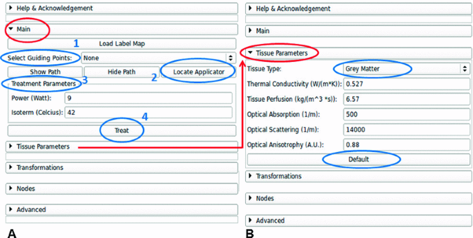
LITTPlan command view has five tab pages. “Main” tab is adequate to perform the operation, while the Tissue Parameters can be modified on the corresponding tab. The optional “Transformations” and “Nodes” tabs are used to rotate and translate the laser applicator, segmentation, 3D model, etc. “Advanced” tab offers extra functionality, e.g., numbering segmentation labels, setting the working folder and setting additional parameters
Fig. 4 
A snapshot of LITTPlan module. On the left is the user command view with the tab pages to plan the operation as well as loading data and processing tools. Right side has four views; three cardinal anatomical planes with registered label maps (segmentations) at the bottom, and a 3D view at the top. User can interact with the mouse to visualize data and models and to position guiding points and applicator(s) as well as to decide an optimum path for the intervention
Table 1 Default tissue parameters -
2.
Locate applicator As seen in Fig. 4, a linear path from the entrance point to the target points is created. A cylindrical model of the laser applicator is then overlaid along this path. The location may be adjusted as needed through manipulation of the fiducial objects.
-
3.
Set treatment parameters User sets laser power in terms of Watts and the isotherm(s) to be calculated in degrees celsius. The provided default values for tissue (i.e., gray/white matter, CSF, tumor, vessel, edema, healthy tissue) parameters can also be adjusted at this step as needed using the interface. Once all the parameters are entered from GUI, “Treat” button can be clicked.
-
4.
Treat All the parameters are read from GUI and sent to the bioheat transfer solver via aforementioned input file. The solution technique for the bioheat transfer returns a 3D isosurface of the tissue damage zone. The 3D damage zone is registered onto MRI and displayed on the GUI (as depicted in Fig. 5 with purple color).


Once the simulation has been completed, the Slicer GUI may be used to save tissue damage as DICOM images for transfer back to an imaging database [26].

An example isotherm simulation, for \(57\,^{\circ }\hbox {C}\) with the power of 10 W, fused on the tissue. a Axial, b Sagittal, c Combined views show the calculated heat (purple)
Steady-state Pennes Bioheat Equation
The LITTPlan module may communicate with a variety of solution techniques for providing estimates of the thermal damage. In particular, we interfaced the LITTPlan module to a steady-state finite element solver of the Pennes Bioheat Equation to simulate the induced heating and expected tissue damage. Bioheat transfer processes in living tissues are significantly influenced by convective heat exchange in the form of blood perfusion through the vascular network. When there is a significant difference between the temperature of the blood and the tissue through which it flows, convective heat transport will occur, altering the temperatures of both the blood and the tissue. The steady-state Pennes’ bioheat equation includes a convective heat transfer term [33] that is proportional to the difference between the local tissue temperature \(T(^{\circ }\hbox {C})\) and the arterial (core) temperature \(T_a(^{\circ }\hbox {C})\) as shown in Eq. 1:
where \({\varvec{k}}\!=\!\hbox {thermal conductivity of tissue}\, (\hbox {Wm}^{-1}\,\hbox {K}^{-1}),\, {{\varvec{q}}}_{\varvec{i}}\!=\! \hbox {Cartesian coordinates (m)},\,w \!=\!\hbox {blood flow} (\hbox {kgm}^{-3}\hbox {s}^{-1})\, {{\varvec{C}}}_{\varvec{b}}= \hbox {specific heat of material}\,(\hbox {Jkg}^{-1}\,^{\circ }\hbox {C}^{-1})\) and \({\varvec{P}}=\) power deposited per unit volume by the laser (\(\hbox {Wm}^{-3}\)).
Estimates for initial bioheat parameters were based on the literature values for the anatomy of interest, Table 1 [31, 32, 34]. Steady-state temperature was calculated, and resulting isotherm estimates of damage were registered as overlays on the treatment planning images. Given the time temperature histories characteristic of laser ablation, the \(57\,^{\circ }\hbox {C}\) isotherm can be used as the threshold to adequately capture damage accrual [31–34]. In other words, we employ the \(57\,^{\circ }\hbox {C}\) isotherm as a surrogate defining the maximum amount of tissue that can be ablated assuming the laser is run until steady-state conditions. Figure 6 shows different components of finite element solution workflow.

The workflow for the finite element solution and Pennes’ bioheat equation
Experimental workflow
The presented pipeline was applied retrospectively to data obtained from five patients during MRgLITT (980 nm laser applicator). First, for each patient, pretreatment MRI data were loaded to Slicer, and the target tissue as well as the surrounding critical structures was segmented semi-automatically using Slicer’s GrowCut algorithm. GrowCut is an efficient algorithm that is based on region growing with cellular automata and can work with a few pixels scribbled in the region of interest by the user and iteratively extracts the foreground and background [35]. The segmentation results of gray matter, white matter, ventricles, and tumor were saved as volumetric label map data. Second, the laser applicator was virtually located, where the actual applicator had been located, by selecting two guiding points, i.e., entrance and target points, represented with aforementioned fiducial markers. The maximum laser power recorded from the delivered therapy was input into the steady-state solver (listed in Table 2). Default tissue parameters were set from the GUI and used as input to the steady-state simulation as well. The isosurface of the \(57\,^{\circ }\hbox {C}\) damage zone predicted by the steady-state solver is overlaid onto the MRI planning data as shown in Fig. 5.
Results
For each patient, the total time to initialize, run, and visualize the simulation registered on MRI was \(<\)5 min. Initialization step included basic environment setup and image segmentation. The whole segmentation process took \(<\)3 min per patient, while each independent realization of the steady-state simulation took \(<\)30 s. Figure 7 shows an example oblique MRI slice acquired during the treatment of the first patient who had been diagnosed with brain metastases (melanoma). This slice was selected in a way that it can show the central long axis cross-section of the laser applicator, the keyhole drilled on the skull, and the maximum amount of tumor and the heating. In this figure, (a) shows the magnitude image of the selected slice, whereas (b) has the temperature image at the hottest time point. Figure 7c, d show zoomed ablation region with the simulated isotherm volume and the corresponding contour projected on the slice to compare with the MRTI output, respectively. Here, the simulation isocontour encircles the maximum region predicted to be ablated, whereas MRTI contour shows the tissue that actually reached the assumed ablation temperature. It was observed that the correspondence between simulation and the real ablation was significant as listed in Table 2. The mean and standard deviation for Hausdorff distance [36] was 2.0 and 0.4 mm between two contours, whereas the mean Dice similarity coefficient (DSC) was 0.93 \((\sigma =0.026)\). The “Coverage” area, which was reported to complement the DSC in this table, denotes the overlap between the areas defined by simulation and MRTI contours, i.e., it is the area of the actual heating that remains within the boundaries of the simulation contour. The minor errors in simulation can be due to segmentation and manual registration inaccuracies as well as the expected uncertainties from MRTI measurements, probe location, fluence, convective, or conductive properties.

a Intraoperative oblique MRI slice showing the tumor and the laser applicator; b MRTI image at the same slice with the hottest time point; c Zoomed into the ablation region with the simulation isosurface registered; d Intersection of the simulation with the slice is created as the isocontour (magenta) of \(57\,^{\circ }\hbox {C}\) for comparison with its corresponding MRTI counterpart (black)
Conclusions and future work
The presented efforts demonstrate the feasibility of incorporating MRI-based predictions of bioheat transfer into an interactive open-source virtual planning environment within a time frame determined by the bioheat transfer solver. The software system presented herein may facilitate MRgLITT planning, within complex scenarios, while simultaneously avoiding damaging critical structures such as the thalamus, mamilothalamic tracts, and fornices. If the actual applicator placement differs from the planned trajectory during surgery, the planning module enables the surgeon to reassess the ablation, with respect to the new location, and decide if it still covers the target or needs repositioning. This knowledge further enables the clinician to refine expectations about achievable ablation and avoids accidental overtreatment as well as allowing the surgeon to determine if the ablation covers the targeted lesion without affecting surrounding tissue and if tails of the tumor are left untreated with the current applicator placement (Fig. 8). The 3D environment for planning the procedure presents opportunities for patient selection and optimizing treatment approach as well as integration with established neuronavigation systems such as Brainsuite (BrainLAB, Inc) via OpenIGTLink. Future work includes a critical study of the tradeoff between computational efficiency and accuracy for a variety of transient, steady-state, and probabilistic bioheat solvers that may be interfaced with the LITTPlan module.

A Multiple ablation example is depicted; a Two target points are selected on the tumor; b Laser applicator is placed to one of the points; c First ablation is simulated; d Second ablation is simulated
References
Stafford RJ, Fuentes D, ElliottAA Weinberg JS, Ahrar K (2010) Laser-induced thermal therapy for tumor ablation. Crit Rev Biomed Eng 38:79–100
Denis de Senneville B, Quesson B, Moonen CT (2005) Magnetic resonance temperature imaging. Int J Hyperth 21:515–531
Rieke V, Butts Pauly K (2008) MR thermometry. J Magn Reason Imaging 27:376–390
Dewhirst MW, Viglianti BL, Lora-Michiels M, Hanson M, Hoopes PJ (2003) Basic principles of thermal dosimetry and thermal thresholds for tissue damage from hyperthermia. Int J Hyperth 19:267–294
McDannold N, Tempany CM, Fennessy FM, So MJ, Rybicki FJ, Stewart EA et al (2006) Uterine leiomyomas: MR imaging-based thermometry and thermal dosimetry during focused ultrasound thermal ablation. Radiology 240:263–272
McNichols RJ, Kangasniemi M, Gowda A, Bankson JA, Price RE, Hazle JD (2004) Technical developments for cerebral thermal treatment: water-cooled diffusing laser fibre tips and temperature-sensitive MRI using intersecting image planes. Int J Hyperth 20:45–56
Schulze PC, Vitzthum HE, Goldammer A, Schneider JP, Schober R (2004) Laser-induced thermotherapy of neoplastic lesions in the brain-underlying tissue alterations, MRI-monitoring and clinical applicability. Acta Neurochir (Wien) 146:803–812
Schwarzmaier HJ, Eickmeyer F, von Tempelhoff W, Fiedler VU, Niehoff H, Ulrich SD et al (2006) MR-guided laser-induced interstitial thermotherapy of recurrent glioblastoma multiforme: preliminary results in 16 patients. Eur J Radiol 59:208–215
Paiva MB, Bublik M, Castro DJ, Udewitz M, Wang MB, Kowalski LP et al (2005) Intratumor injections of cisplatin and laser thermal therapy for palliative treatment of recurrent cancer. Photomed Laser Surg 23:531–535
Schwarzmaier H-J, Eickmeyer F, Fiedler VU, Ulrich F (2002) Basic principles of laser induced interstitial thermotherapy in brain tumors. Med Laser Appl 17:147–158
Schwarzmaier H-J, Eickmeyer F, von Tempelhoff W, Fiedler VU, Niehoff H, Ulrich SD et al (2006) MR-guided laser-induced interstitial thermotherapy of recurrent glioblastoma multiforme: preliminary results in 16 patients. Eur J Radiol 59:208–215
Carpentier A, McNichols RJ, Stafford RJ, Guichard JP, Reizine D, Delaloge S et al (2011) Laser thermal therapy: real-time MRI-guided and computer-controlled procedures for metastatic brain tumors. Lasers Surg Med 43:943–950
Curry DJ, Gowda A, McNichols RJ, Wilfong AA (2012) MR-guided stereotactic laser ablation of epileptogenic foci in children. Epilepsy Behav 24:408–414
Bondarenko E, Iur’eva E, Zykov V, Alekseeva N (1997) The laser therapy of children with Tourette’s syndrome. Zhurnal nevrologii i psikhiatrii imeni SS Korsakova/Ministerstvo zdravookhraneniia i meditsinskoĭ promyshlennosti Rossiĭskoĭ Federatsii. Vserossiĭskoe obshchestvo nevrologov [i] Vserossiĭskoe obshchestvo psikhiatrov 97:29
Rahmathulla G, Recinos PF, Valerio JE, Chao S, Barnett GH (2012) Laser interstitial thermal therapy for focal cerebral radiation necrosis: a case report and literature review. Stereotact Funct Neurosurg 90:192–200
Beccaria K, Canney MS, Carpentier AC (2012) Magnetic resonance-guided laser interstitial thermal therapy for brain tumors. In: Hayat MA (ed) Tumors of the central nervous system. Springer, Amsterdam, pp 173–185
Carpentier A, Chauvet D, Reina V, Beccaria K, Leclerq D, McNichols RJ et al (2012) MR-guided laser-induced thermal therapy (LITT) for recurrent glioblastomas. Lasers Surg Med 44:361–368
Hawasli AH, Ray WZ, Murphy RK, Dacey RG Jr, Leuthardt EC (2012) Magnetic resonance imaging-guided focused laser interstitial thermal therapy for subinsular metastatic adenocarcinoma: technical case report. Neurosurgery 70:332–338
Jones S, Barnett G, Sunshine JL, Griswold M, Sloan A, Phillips MD, Tyc R, Torchia M (2009) First human application of laser interstitial thermal therapy in GBM using MR guided autolitt system. In: Proceedings of the 17th scientific meeting, international society for magnetic resonance in medicine
Sunshine J, Sandhu G, Sloan A, Griswold M (2012) O-030 Laser thermotherapy of malignant brain lesions using MRI for needle guidance and real-time temperature mapping. J NeuroInterv Surg 4:A17–A17
Fahrenholtz S, Fuentes D, Stafford R, Hazle J (2012) Uncertainty quantification by generalized polynomial chaos for MR-guided laser induced thermal therapy. Med Phys 39:3857
Topaloglu U, Yan Y, Novak P, Spring P, Suen J, Shafirstein G, (2008) Virtual thermal ablation in the head and neck using comsol MultiPhysics. In: Proceedings of the COMSOL conference 2008, pp 1–7
Neufeld E, Paulides MM et al (2012) Numerical modeling for simulation and treatment planning of thermal therapy. In: Moros EG (ed) Physics of thermal therapy: fundamentals and clinical applications. CRC Press, Boca Raton
Kirk BS, Peterson JW, Stogner RH, Carey GF (2006) libMesh: a C++ library for parallel adaptive mesh refinement/coarsening simulations. Eng Comput 22:237–254
Tokuda J, Fischer GS, Papademetris X, Yaniv Z, Ibanez L, Cheng P et al (2009) OpenIGTLink: an open network protocol for image-guided therapy environment. Int J Med Robotics Comput Assist Surg 5:423–434
Pieper S, Halle M, Kikinis R (2004) 3D Slicer. In: Biomedical imaging: nano to macro, 2004. IEEE international symposium on, vol 1, pp 632–635
Kikinis R, Pieper S (2011) 3D Slicer as a tool for interactive brain tumor segmentation. Conf Proc IEEE Eng Med Biol Soc 4:6982–6984
Pinter C, Lasso A, Wang A, Jaffray D, Fichtinger G (2012) SlicerRT: radiation therapy research toolkit for 3D Slicer. Med Phys 39:6332
Available: http://www.slicer.org/pages/Slicer_Community
Fedorov A, Beichel R, Kalpathy-Cramer J, Finet J, Fillion-Robin J-C, Pujol S et al (2012) 3D Slicer as an image computing platform for the Quantitative Imaging Network. Magn Reson Imaging 30:1323–1341
Welch AJ, Van Gemert MJ (2010) Optical-thermal response of laser-irradiated tissue. Springer, Berlin
Welch A (1984) The thermal response of laser irradiated tissue. Quantum Electron IEEE J 20:1471–1481
Bergman TL, Lavine AS, Incropera, FP DeWitt D (2011) Introduction to heat transfer, 6th edn. Wiley, Hoboken
Fuentes D, Yusheng F, Elliott A, Shetty A, McNichols RJ, Oden JT et al (2010) Adaptive real-time bioheat transfer models for computer-driven MR-guided laser induced thermal therapy. Biomed Eng IEEE Trans 57:1024–1030
Vezhnevets V, Konouchine V (2005) GrowCut: interactive multi-label ND image segmentation by cellular automata. In: Proceedings of graphicon, pp 150–156
Rockafellar RT, Wets RJ-B (1998) Variational analysis: Grundlehren der mathematischen wissenschaften, vol 317. Springer, Newyork
Acknowledgments
This research is supported in part by the MD Anderson Cancer Center Support Grant CA016672 and the National Institutes of Health (NIH) award 1R21EB010196-01 and Apache Corporation. All opinions, findings, conclusions, or recommendations expressed in this work are those of the authors and do not necessarily reflect the views of our sponsors. The data were acquired in part from Visualase Inc. (Houston, TX, USA). Conflict of interest None
Author information
Authors and Affiliations
Corresponding author
Rights and permissions
About this article
Cite this article
Yeniaras, E., Fuentes, D.T., Fahrenholtz, S.J. et al. Design and initial evaluation of a treatment planning software system for MRI-guided laser ablation in the brain. Int J CARS 9, 659–667 (2014). https://doi.org/10.1007/s11548-013-0948-x
Received:
Accepted:
Published:
Issue Date:
DOI: https://doi.org/10.1007/s11548-013-0948-x