
Abstract
A new method, called augmented blanket with rotating grid (ABRG), has been proposed in our recent work on characterizing roughness and directionality of self-structured surface textures. This is the first method that calculates fractal dimensions (FDs) at individual scales and directions for the entire surface image data and does not require the data to be Brownian fractal. However, before the ABRG method can be used in real applications, effects of atomic force microscope (AFM) imaging conditions on FDs need to be evaluated first. In this paper, computer-generated AFM images with three different resolutions, 48 combinations of tip radii and cone angles, and 15 noise levels were used in the tests. The images represent isotropic self-structured surface textures with small, medium and large motif sizes, and anisotropic surfaces exhibiting two dominating directions. For isotropic surfaces, the ABRG method is not significantly affected (i.e. FDs changes <5 %) by image resolution, tip size (for surfaces with large motifs) and noise (except the level above 8 %). For anisotropic surfaces, the method exhibits large changes in FDs (up to −34 %). The results obtained show that the ABRG method can be effective in analysing the AFM images of self-structured surface textures. However, some precautions should be taken with anisotropic and isotropic surfaces with small motifs.
1 Introduction
Self-structured surface textures are generated by self-assembling rules of molecules on a substrate surface. The self-assembly process is driven by complicated intermolecular and molecular-substrate forces and the resulting textures exhibit recurring topographical features, called motifs, of various shapes, sizes and orientations distributed on the surface in one or more layers. Due to nanoscale dimensions of the motifs and their strong bonding with substrate surface, these textures have many applications in engineering and medicine. For example, they can be used to improve tribological characteristics of micromechanical systems such as micromotors [1], regulate cell membrane penetration of nanoparticles in medical drug delivery systems [2, 3], enhance Raman scattering for monitoring of intracellular events [4], and increase efficiency of optical data-storage devices [5].
For the image acquisition of self-structured surfaces optical [6], scanning electron (SEM) [7], atomic force (AFM), scanning tunnelling (STM) [8], Fourier transform infrared spectroscopy (FTIS) [9] microscopes have been used. AFM is the method of choice [6, 8, 10–12] since it operates in ambient conditions, can image samples in liquid, gas and vacuum environments [13], requires minimal sample preparations, and provides real 3D surface topography data [13, 14].
Roughness of the surfaces has been quantified using basic parameters such as average roughness (R a) [15, 16], root-mean-square roughness (RMS) [7, 12, 16, 17], maximum peak roughness (R max) [16]. Fourier transform [18, 19], box-counting [20] or slit-island methods [21] are also used. However, these methods and parameters calculated provide only a limited information about surface texture. The reason is that they do not quantify surface roughness at different scales and directions. To overcome the limitation, directional fractal signature (DFS) methods have been developed [22]. They quantify surface roughness and directionality using fractal dimensions (FDs) calculated at individual scales and directions. Analysing surface textures using FS is of practical significance since self-structured surfaces are not ideal fractals, i.e. their roughness and directionality vary with scale [23]. Five DFS methods are available, i.e.: FS Hurst orientation transform (FSHOT), variance orientation transform (VOT), blanket with rotating grid (BRG) [22], augmented BRG (ABRG) and blanket with shearing image (BSI) [23]. Previous study showed that the VOT and FSHOT methods are not suitable in the characterization of self-structured surface textures, since the methods require surfaces to be fractal Brownian [23]. In the past study, the ABRG, BRG and BSI methods were evaluated in the measurements of surface roughness and directionality of self-structured surfaces, their capacity for quantifying multi-patterned textures and ability to detect differences between real self-structured surfaces generated with differently polarized laser beams. Images of computer-generated and real self-structured surfaces were used. Results showed that the ABRG is the best performing method. However, if the method is to be of use to real applications, the effects of AFM imaging conditions such as image resolution, tip size and noise on FDs calculated would need to be studied and assessed first.
In the current study, this problem is addressed by evaluating the effects of the AFM imaging conditions using surface images generated by means of a motif-based texture generator (MTG) [23]. The images represent three self-structured isotropic surfaces with motif sizes of ~250, ~350 and ~500 nm, and two anisotropic surfaces exhibiting two dominating directions (i.e. 50° and 140°). The surfaces have a coverage area of 10 μm × 10 μm with a height range of 250 nm. The sizes of motifs, area and range used in this study are similar to those found in real self-structured surfaces [18, 19]. The MTG and image processing techniques were used to construct databases of images with three different resolutions, 48 combinations of tip radii and cone angles, and 15 noise levels.
2 Methods and Materials
2.1 ABRG Method
In the method, FSs, i.e. FDs at individual scales, are calculated in all possible directions in the following steps (more details are given in [23]):
-
1.
An original image is covered by a rotating grid (Fig. 1a, b).
Fig. 1 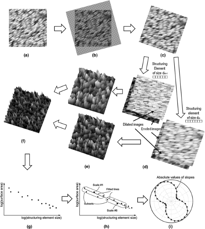
A schematic illustration of the ABRG method. a An original image, b a rotating grid superimposed on the image, c a rotated image, d dilated and eroded images using structuring elements of sizes d m and d m−1, e surface volumes, f a surface area, g a log–log plot, h lines fitted to the subsets and i a rose plot of absolute values of slopes
-
2.
The grid rotates around its centre over the image by predefined directions (between 0° to 180° in steps of 10°) and image pixels covered by it are copied into a matrix, i.e. a new image (Fig. 1c). The size of rotating grid is automatically adjusted for each direction to ensure that all image pixels are covered.
-
3.
Dilated and eroded versions of the matrix are obtained using line structuring elements (SEs) of different sizes (Fig. 1d). Sizes of SEs rank from 3 to 16 pixels.
-
4.
For each direction, surface volumes enclosed between the dilated and eroded images are calculated (Fig. 1e), and then differences between the volumes at two consecutive SE sizes are used to obtain surface areas (Fig. 1f).
-
5.
The areas obtained are plotted against SE sizes in log–log coordinates (Fig. 1g).
-
6.
The plot data points are divided into overlapping sets of five points and a line is fitted to each set (Fig. 1h). The SE size associated with the middle point in each set represents an individual scale.
-
7.
The absolute values of slopes obtained are plotted against direction in polar coordinates (Fig. 1i). The slope S relates to FD as 2 − S. In total there are nine rose plots, i.e. one plot for each scale.

As an example, the ABRG method was applied to AFM images of isotropic and anisotropic self-structured surface textures shown in Fig. 2. The isotropic surface (Fig. 2a) was obtained through the electron-beam evaporation of a gold film [24], while the anisotropic surface (Fig. 2b) was the result of laser irradiation of a molecular azo glass film [19]. The resulting rose plots of slopes (Fig. 3) obtained for the isotropic surface approximate a circle at all scales. This indicates that roughness of the surface does not change considerably with direction. On the contrary, the rose plots obtained for the anisotropic surface show rapid changes of slope values with direction at all scales, i.e. changes in roughness with direction and scale.


Rose plots of slopes at nine scales obtained by means of the ABRG method for the isotropic (asterisk) and anisotropic (circle) self-structured surface texture images shown in Fig. 2a, b, respectively. For the isotropic surface, nine scale numbers correspond to 27.3–72.8 nm in steps of 4.55 nm, and for the anisotropic surface they correspond to 203.4–542.4 nm in steps of 33.9 nm
2.2 MTG
The generator produces texture images of artificial self-structured surfaces [23]. This is achieved by a placement of half-ellipsoid motifs on an empty image in the following four steps:
-
1.
An empty image (i.e. all grey-scale level values are set to zero) is generated and initial coordinates of centres of motifs are defined. The vertical and horizontal distances between centres are denoted by s x and s y , respectively. Each centre is translated in the horizontal and vertical directions by a random number of pixels, and then rotated around the centre of the image by a given angle β. The translation in the two directions is parameterized by a 1 and a 2 scaling factors. Examples of the centres obtained are shown in Fig. 4a.
Fig. 4 
A schematic illustration of the MTG. a An empty image (all pixels set to zero) with centres of motifs (white dots), b motifs placed at the centres, c concatenated motifs and d a cropped image
-
2.
Motifs with given radii (r 1, r 2 in the horizontal and vertical directions, and r 3 in the direction perpendicular to surface plane) are generated and then located at the centres (Fig. 4b).
-
3.
Motifs that overlap each other are concatenated (Fig. 4c).
-
4.
Image of motifs obtained is cropped to a predefined size (Fig. 4d).

2.3 AFM Image Simulation
AFM images are the results of the convolution of surface topography and tip geometry [14]. In the current study, the images were generated through a dilation of artificially generated self-structured surfaces using conically shaped tips of different sizes [25]. Conical tips were chosen since they are axisymmetric. Thus, the image dilation affects surface texture features equally in all directions.
A cross section of the conical tip is shown in Fig. 5a. The tip is a result of the concatenation of a sphere with radius r and a cone with half-cone angle θ. Tip height \( t_{h} \) is given by the following expression:
where d is the distance from the tip apex O,

a Cross section of a geometrical model of a conical tip characterized by radius r and cone angle θ, and b example of a reflected (by tip apex) conical 3D tip model generated with r = 30 nm and θ = 45°
For the dilation of surface, the 3D tip geometry is represented as a 2D matrix of heights \( {\mathbf{T}} \) as follows:
-
1.
An empty matrix \( {\mathbf{T}} \) of size N × N is generated, where \( N = {\text{ceil}}\left( {2*\tan {{\theta}}*\left( {h + \left| {\text{OD}} \right|} \right)} \right) \) and h is the range of surface heights. This ensures that tip heights generated cover the entire range h.
-
2.
Let j = 1.
-
2.1
Let i = 1.
-
2.2
x and y coordinates are calculated in such a way that the tip apex is located in the middle of \( {\mathbf{T}} \), i.e. x = i − N/2 − 0.5 and y = j − N/2 − 0.5.
-
2.3
Distance d of the point (x,y) from the tip apex is calculated, i.e. \( d = \sqrt {x^{2} + y^{2} } \).
-
2.4
If \( d \le N/2 \) then the tip height at the distance d is calculated and stored in the matrix \( {\mathbf{T}} \), i.e. \( {\mathbf{T}}_{j,i} = t_{h} (d) \).
-
2.5
i = i + 1 and go to step 2.2 unless i > N.
-
2.1
-
3.
j = j + 1 and go to step 2.1 unless j > N.
-
4.
The tip is reflected around its apex: \( {\mathbf{T}}_{i,j} = - {\mathbf{T}}_{j,i} \) for all i and j.
An example of a tip generated for r = 30 nm and θ = 45° is shown in Fig. 5b. h was set to 250 nm. A resolution of the matrix \( {\mathbf{T}} \) was assumed to be 1 nm, which is a typical value used in AFM [26].
3 Results
3.1 Effects of Image Resolution
AFM can produce images of different sizes (i.e. different image resolutions) for the same area of self-structured surfaces. Effects of image resolution on FDs calculated by the ABRG method were, therefore, studied. Isotropic and anisotropic surface images with sizes of 512 × 512, 256 × 256 and 128 × 128 pixels were used. These size images of surfaces are typical for AFM.
Images of three isotropic self-structured surfaces were generated with increasing sizes of motifs, i.e. small (~250 nm), medium (~350 nm) and large (~500 nm) sizes. Each surface was represented as 512 × 512 pixel image with 256 grey-scale levels. In the MTG, a 1 and a 2 were equalled to 1, r 3 was set individually for each motif as a random integer number between 0 and 255, and β was set to 0°. To generate small, medium and large motifs r 1 = r 2 = s x = s y were set to 6.4, 9 and 13, respectively. The anisotropic surface with 50° and 140° dominating directions was also generated. For the surface, the following set-up was used: β = 50°, r 1 = r 2 = s x = s y = 6, a 1 = a 2 = 0. Also, for each motif r 3 was selected for groups of four motifs as a random integer number between 0 and 255 and every fifth row of the initial centre coordinates of motifs was deleted. For all surfaces used in this study, the original image of 512 × 512 pixel was reduced to 256 × 256 and 128 × 128 pixels using the block averaging [27]. The generation process of surfaces was repeated 50 times. In total, 600 (= 4 × 50 × 3) images were obtained, i.e. for each resolution 50 images per surface. Examples of isotropic and anisotropic surface images generated with different resolutions are shown in Fig. 6.


Examples of self-structured surface texture images of sizes a, d, g, j 512 × 512 pixels; b, e, h, k 256 × 256 pixels and c, f, j, l 128 × 128 pixels. Surfaces a, d, g are isotropic with small, medium and large motifs, respectively, and surface j is anisotropic with 50° and 140° dominating directions
The ABRG method was first applied to the images of isotropic surfaces with small motifs. For each image resolution, mean FD values were calculated at individual scales in all directions. Scales used by 512 × 512, 256 × 256 and 128 × 128 pixel images are different, i.e. 117.2–273.4 nm in steps of 19.5 nm, 234.4–546.9 nm in steps of 39.1 nm, and 468.8–1093.6 nm in steps of 78.1 nm, respectively. Consequently, 256 × 256 pixel images share two scales with the largest (i.e. 234.4 and 273.4 nm) and smallest (i.e. 468.8 and 546.9 nm) images. For the shared scales, percentage differences between mean FD values obtained for 512 × 512 and 256 × 256 pixel images, and between 128 × 128 and 256 × 256 pixel images were calculated. This procedure was repeated for the remaining surfaces. The differences calculated were displayed against directions in polar coordinates as rose plots (Figs. 7, 8). A grey colour ring represents values between −5 and 5 %.

Effect of image resolution on FDs calculated by the ABRG method for the isotropic self-structured surfaces with small (asterisk), medium (square) and large (triangle) motifs. The markers represent percentage differences between mean values of FDs obtained for a, b 512 × 512 and 256 × 256; and c, d 128 × 128 and 256 × 256 pixel images. The dotted circle denotes 0 % difference and the grey colour ring area represents changes between −5 and 5 %

Effect of image resolution on FDs calculated by the ABRG method for anisotropic self-structured surfaces with 50° and 140° dominating directions. The markers represent percentage differences between mean values of FDs obtained for a, b 512 × 512 and 256 × 256 and c, d 128 × 128 and 256 × 256 pixel images. The dotted circle denotes 0 % difference and the grey colour ring area represents changes between −5 and 5 %
For the isotropic surfaces the percentage differences in mean FD values stay within the grey ring (Fig. 7). Specifically, for the surface with small motifs, the mean FDs calculated for 512 × 512 (128 × 128) pixel images were smaller up to −4.4 % (higher up to 2.2 %) than those calculated for 256 × 256 pixel images. For the surfaces with medium and large motifs, the differences were less than 4.1 %. For the anisotropic surfaces, the differences also stay within the ring, except directions about 140° where they are about −30 % (Fig. 8).
3.2 Effects of Tip Size
To study the effects of tip size, AFM images of the isotropic and anisotropic surfaces were generated for different tip radii r (i.e. 2, 5, 10, 20, 40, 60, 80 and 100 nm) and cone angles θ (i.e. 5°, 15°, 30°, 35°, 40° and 45°). The radii and angles represent a wide range of AFM tips; ranking from the ultra sharp with high aspect ratio (i.e. r = 2 nm, θ = 5°) to the wide with low aspect ratio (i.e. r = 100 nm, θ = 45°). The generation of images was conducted in following several steps:
-
1.
The radius r and cone angle θ are selected.
-
2.
Using MTG, 11,264 × 11,264 pixel and 256 grey-scale levels images of self-structured surfaces with small, medium and large motifs are generated. The pixel size of 1 nm is assumed. MTG parameters are taken from the previous section, with two exceptions, i.e. for the isotropic surfaces r 1 = r 2 = s x = s y are set to 125, 175 and 250, respectively, and for the anisotropic surface r 1 = r 2 = s x = s y = 120.
-
3.
A 2D matrix of tip heights is constructed for the selected r and θ.
-
4.
Each surface image is dilated using the 2D matrix. To eliminate the edge effects, the dilation is performed over a 10,240 × 10,240 pixel area located in the centre of the original surface image.
-
5.
From the area selected on the original image every 40th pixel in the horizontal and vertical directions is copied into an empty image of size 256 × 256 pixels (called an ideal image).
-
6.
Every 40th pixel is also copied from the dilated area into an empty image (called an AFM image).
-
7.
Steps 1 to 6 are repeated 50 times for all possible combinations of the radii and angles (i.e. 48 combinations). This result in 9,600 (= 4 × 48 × 50) AFM and 200 (= 4 × 50) ideal images, i.e. 2400 AFM and 50 ideal images per surface.
As an example, the AFM and ideal images of isotropic and anisotropic surfaces obtained for r = 100 nm and θ = 45° are shown in Fig. 9.

Examples of a, c, e, g ideal and b, d, f, h AFM images (r = 100 nm and θ = 45°) of self-structured surface textures. Surfaces a, c, e are isotropic with small, medium and large motifs, respectively, and surface g is anisotropic with 50° and 140° dominating directions
The ABRG method was applied to the images generated. For each possible combination of r and θ, percentage differences between mean FD values obtained for the AFM and corresponding ideal image were calculated. As an example, rose plots of the differences obtained for isotropic surfaces with small motifs and anisotropic surfaces at different tip radii and cone angle of 5° are shown in Figs. 10 and 11, respectively. For the isotropic surfaces, the plots show that FDs decrease with tip radius. For surfaces with small (medium) motifs the differences were largest, i.e. up to −8 % (−6 %), at small scales. For surfaces with large motifs, differences were below −5 %. Anisotropic surfaces had the differences greater than −5 % at all scales (Fig. 11), with the largest value of approximately −34 % at the largest scale in about 140° direction.

Effect of tip size on FDs calculated by the ABRG method for the isotropic self-structured surfaces with small motifs. The markers represent percentage differences between mean FD values calculated for AFM images obtained using tip with cone angle θ = 5° and radius r = 2 nm (asterisk), 5 nm (square), 20 nm (triangle), 40 nm (circle), 60 nm (rhombus), 100 nm (plus), and the ideal images. The grey colour ring area represents changes between −5 and 0 %

Effect of tip size on FDs calculated by the ABRG method for the anisotropic self-structured surfaces with 50° and 140° dominating directions. The markers represent percentage differences between mean FD values calculated for AFM images obtained using tip with cone angle θ = 5° and radius r = 2 nm (asterisk), 5 nm (square), 20 nm (triangle), 40 nm (circle), 60 nm (rhombus), 100 nm (plus), and the ideal images. The grey colour ring area represents changes between −5 and 0 %
Rose plots of the differences (figures are not shown) were also obtained for cone angles of 15°, 30°, 35°, 40° and 45° and they were similar to those of the 5° cone angle.
3.3 Effects of Noise
AFM images contain instrumental noise originated from mechanical vibrations and electrical signal fluctuation. This noise follows approximately a Gaussian distribution with zero mean [28]. Therefore, the Gaussian noise was added to the images of self-structured surfaces and its effects on FDs calculated were investigated.
256 × 256 pixel images of the self-structured surfaces were generated using the MTG as described in Sect. 3.1. For the isotropic surfaces r 1 = r 2 = s x = s y were set to 3.2, 4.5 and 6.5, respectively, and for the anisotropic surface r 1 = r 2 = s x = s y = 3. For each surface 15 images were generated by adding Gaussian noise at different level, i.e. Gaussian noise with a standard deviation increasing from 1 to 15 % in steps of 1 % of the maximal grey-scale level value. The noise generation process was repeated 50 times. As a result, 3,000 (= 4 × 15 × 50) noise images were obtained, i.e. 200 per each noise level. Examples of isotropic and anisotropic surfaces without and with noise at level of 15 % are shown in Fig. 12.

Examples of self-structured surface texture images a, c, e, g without and b, d, f, h with noise level of 15 %. Surfaces a, c, e are isotropic with small, medium and large motifs, respectively, and surface g is anisotropic with 50° and 140° dominating directions
For each noise level, percentage differences in mean FD values between images with and without noise were calculated. As an example, rose plots of the differences for isotropic surfaces with large motifs are shown in Fig. 13. For the isotropic surfaces, FDs calculated increase proportionally to the noise level. The differences in mean FDs were higher than 5 % for noise levels of 13 % (small motif), 10 % (medium motif) and 9 % (large motif). Isotropic surfaces with medium and large motifs exhibited the largest differences (~13 %) at the first scale. For anisotropic surfaces (figure not shown), the differences in mean FDs are above 5 % for noise level of 4 %; with the largest value of ~26 % in directions around 140°.

Effect of Gaussian noise on FDs calculated by the ABRG method for the isotropic self-structured surfaces with large motifs. Markers represent percentage differences between mean FD values calculated for images with and without noise at noise levels of 1 % (asterisk), 7 % (square), 9 % (triangle), 11 % nm (circle), 13 % (rhombus), and 15 % (plus). The grey colour ring area represents changes between 0 and 5 %
4 Discussion
In this study, effects of AFM image resolution, tip size and noise on the performance of the ABRG method were evaluated. Images of isotropic self-structured surfaces with increasing motif sizes and anisotropic surfaces exhibiting two dominating directions were generated by the MTG. For the isotropic surfaces, the ABRG method is not significantly affected (i.e. FDs changes <5 %) by image resolution, tip size (for surfaces with large motifs) and noise (levels below 9 %). For the anisotropic surfaces the method had large changes in FDs, i.e. up to −34 %.
For different image resolutions the isotropic surfaces had small changes in mean FDs (<5 %). This is partially supported by the results obtained in a previous study, where isotropic porphyrin thin film surfaces were imaged using AFM at image resolutions ranking from 128 × 128 to 1,024 × 1,024 pixels [29]. It was found that changes in the RMS roughness do not vary significantly with the image resolution. For anisotropic surfaces, the image resolution has a significant effect on FDs. The differences in FDs were up to −30 %, especially between 128 × 128 and 256 × 256 pixel images in directions about 140°. At these two resolutions the rose plots of slopes were visually examined. Examples of the surface images are shown in Fig. 6k, l. For the small resolution, 140° dominating direction is the least visible. This is because gaps between stripes of motifs on the 128 × 128 pixel images are blurred and not clearly defined. Subsequently, at low resolution anisotropic surfaces appear to be more isotropic. Hence, AFM images of anisotropic surfaces should not be acquired with resolution lower than 256 × 256 pixels.
Tip size affects the values of FDs calculated. As compared to the ideal images, mean FDs decrease for all surfaces. This agrees with other studies [30, 31]. The decrease in FDs can be explained by the fact that the tip–surface convolution smooths fine details of surfaces. The changes of FD values were greater for tip radii than for cone angles. This is because the tip apex, which size is determined by the tip radius, is the main part of a tip that interacts with surface. This has some support from a previous study in which FDs calculated for fractal surface images were virtually constant over a wide range of the AFM tip aspect ratios [32]. FDs calculated for surfaces with small motifs exhibited largest changes in mean FDs (up to −8 %) at the first scale, followed by FDs calculated for surfaces with medium (up to −6 %) and large motifs (up to −5 %). This can be explained by the fact that the tip–surface convolution is a local operation and it mostly targets small scale surface features. Previous study, in which isotropic fractal surface images with known FD were dilated by tips of different radii [30], showed similar results. Specifically, it was found that the changes in FDs are largest for the rough surfaces, i.e. surfaces with high FD. For the anisotropic surfaces, the differences in FDs were largest (about −34 %) in directions of about 140° at the last scale. Visual comparison of AFM images obtained (e.g. Fig. 9g, h) indicates that the gaps between the stripes of motifs are reduced by the broadening of surface features. Subsequently, the surfaces appear more isotropic on AFM images. Thus, knowing that surfaces are isotropic with small motifs or anisotropic would be helpful in the selection of tip sizes for the analyses with the ABRG method.
FDs increase by more than 5 % at noise levels greater than 8 %. For the isotropic surfaces, the largest increases were found for surfaces with large motifs at small scales (~13 %). This is because the noise adds high frequency components to the smooth areas of large motifs. For anisotropic surfaces, noise causes a rapid increase in the surface roughness (up to 26 %) for groups of the smooth motifs aligned in 140°. Therefore, during the AFM image acquisition all precautions should be taken to reduce the noise level.
AFM image quality can be affected by other factors than those studied in the paper. First, cantilevers with high spring constant can damage a surface [33]. If the constant is low poor phase contrast images can be produced [33]. Second factor is incorrect settings of the feedback loop control which maintains the set force between tip and sample. They can cause inaccurate tracking of the surface and introduce high frequency noise [14]. Third factor is the relation between the sizes of a surface feature and the tip radius. If radii of curvature of surface futures are less than double of tip radius, smoothening of fine surface features can be significant [34]. Finally, there are tips with non-symmetrical shapes (e.g. pyramidal or tetrahedral) and they can produce images of surfaces with features whose degree of dilation changes with direction.
Future work would focus on applications of the ABRG method to images of real self-structured surfaces. One application is the analysis of self-structured surface textures generated by laser irradiation of polymer films. This would aim at understanding of the formation process of the surface textures. Relationships between the textures and the laser irradiation conditions (e.g. laser beam wavelength and polarization) are still not fully determined [18, 19]. Attempts made so far are based on the visual assessment of 2D Fourier transform of the surface images [18, 19]. However, this has a limited use since surface details at individual scales and different directions were not quantified. Using the ABRG method this limitation can be overcome.
5 Conclusions
From the work conducted the following conclusions can be drawn:
-
Effects of AFM imaging conditions (i.e. image resolution, tip size and noise) on FDs calculated by the ABRG method were evaluated.
-
Computer-generated images of isotropic self-structured surfaces with increasing motif sizes and anisotropic surfaces with two dominating directions were generated by the MTG.
-
For isotropic surfaces, FDs do not change considerably (<5 %) with image resolution, tip size (for large motifs) and noise (except levels >8 %). For anisotropic surfaces, changes in FDs could be up to −34 %.
-
The results obtained demonstrate that the ABRG method can be effective in the analysis of AFM images of self-structured surfaces, although precautions are needed for surfaces with small motifs and anisotropic surfaces.
References
Maboudian, R., Ashurst, W.R., Carraro, C.: Tribological challenges in micromechanical systems. Tribol. Lett. 12, 95–100 (2002)
Verma, A., Uzun, O., Hu, Y.H., Hu, Y., Han, H.S., Watson, N., Chen, S.L., Irvine, D.J., Stellacci, F.: Surface structure-regulated cell-membrane penetration by monolayer-protected nanoparticles. Nat. Mater. 7, 588–595 (2008)
Pons-Siepermann, I.C., Glotzer, S.C.: Design of patchy particles using quaternary self-assembled monolayers. ACS Nano 6, 3919–3924 (2012)
Klutse, C.K., Mayer, A., Wittkamper, J., Cullum, B.M.: Applications of self-assembled monolayers in surface-enhanced Raman scattering. J. Nanotechnol. 2012, Article ID 319038 (2012)
Ahmadi-Kandjani, S., Barille, R., Dabos-Seignon, S., Nunzi, J.M., Ortyl, E., Kucharski, S.: Self-induced diffraction grating storage in polymer films. Mol. Cryst. Liq. Cryst. 446, 99–109 (2006)
Nakano, M.: Tribological properties of self-assembled monolayers. In: Biresaw, G., Mittal, K. (eds.) Surfactants in Tribology, vol. 2, pp. 3–15. CRC Press, Boca Raton (2011)
Kaufmann, C., Mani, G., Marton, D., Johnson, D., Agrawal, C.M.: Long-term stability of self-assembled monolayers on electropolished L605 cobalt chromium alloy for stent applications. J. Biomed. Mater. Res. B: Appl. Biomater. 98B, 280–289 (2011)
Kudernac, T., Shabelina, N., Mamdouh, W., Hoger, S., De Feyter, S.: STM visualisation of counterions and the effect of charges on self-assembled monolayers of macrocycles. Beilstein J. Nanotechnol. 2, 674–680 (2011)
Hurst, K.M., Ansari, N., Roberts, C.B., Ashurst, W.R.: Self-assembled monolayer-immobilized gold nanoparticles as durable, anti-stiction coatings for MEMS. J. Microelectromech. Syst. 20, 424–435 (2011)
Miyake, K., Hori, Y., Ikeda, T., Asakawa, M., Shimizu, T., Sasaki, S.: Alkyl chain length dependence of the self-organized structure of alkyl-substituted phthalocyanines. Langmuir 24, 4708–4714 (2008)
Miyake, K., Fukuta, M., Asakawa, M., Hori, Y., Ikeda, T., Shimizu, T.: Molecular motion of surface-immobilized double-decker phthalocyanine complexes. J. Am. Chem. Soc. 131, 17808–17813 (2009)
Bhushan, B., Kulkarni, A.V., Koinkar, V.N.: Microtribological characterization of self-assembled and Langmuir–Blodgett monolayers by atomic and friction force microscopy. Langmuir 11, 3189–3198 (1995)
Russell, P., Batchelor, D., Thornton, J.: SEM and AFM: Complementary Techniques for High Resolution Surface Investigations. Bruker Corporation, Billerica (2010)
Eaton, P., West, P.: Atomic Force Microscopy. Oxford University Press, Oxford (2010)
Faucheux, N., Schweiss, R., Lutzow, K., Werner, C., Groth, T.: Self-assembled monolayers with different terminating groups as model substrates for cell adhesion studies. Biomaterials 25, 2721–2730 (2004)
Zhuang, Y.X., Hansen, O., Knieling, T., Wang, C., Rombach, P., Lang, W., Benecke, W., Kehlenbeck, M., Koblitz, J.: Vapor-phase self-assembled monolayers for anti-stiction applications in MEMS. J. Microelectromech. Syst. 16, 1451–1460 (2007)
Losego, M.D., Guske, J.T., Efremenko, A., Maria, J.P., Franzen, S.: Characterizing the molecular order of phosphonic acid self-assembled monolayers on indium tin oxide surfaces. Langmuir 27, 11883–11888 (2011)
Yin, J.J., Ye, G., Wang, X.G.: Self-structured surface patterns on molecular azo glass films induced by laser light irradiation. Langmuir 26, 6755–6761 (2010)
Wang, X.L., Yin, J.J., Wang, X.G.: Photoinduced self-structured surface pattern on a molecular azo glass film: structure-property relationship and wavelength correlation. Langmuir 27, 12666–12676 (2011)
Lam, K.T., Ji, L.W.: Fractal analysis of InGaN self-assemble quantum dots grown by MOCVD. Microelectron. J. 38, 905–909 (2007)
Consolin, N., Leite, F.L., Carvalho, E.R., Venancio, E.C., Vaz, C.M.R., Mattoso, L.H.C.: Study of poly(o-ethoxyaniline) interactions with herbicides and evaluation of conductive polymer potential used in electrochemical sensors. J. Braz. Chem. Soc. 18, 577–584 (2007)
Wolski, M., Podsiadlo, P., Stachowiak, G.W.: Directional fractal signature analysis of trabecular bone: evaluation of different methods to detect early osteoarthritis in knee radiographs. Proc. Inst. Mech. Eng. H 223, 211–236 (2009)
Wolski, M., Podsiadlo, P., Stachowiak, G.W.: Directional fractal signature analysis of self-structured surface textures. Tribol. Lett. 47, 323–340 (2012)
Love, J.C., Estroff, L.A., Kriebel, J.K., Nuzzo, R.G., Whitesides, G.M.: Self-assembled monolayers of thiolates on metals as a form of nanotechnology. Chem. Rev. 105, 1103–1169 (2005)
Villarrubia, J.S.: Algorithms for scanned probe microscope image simulation, surface reconstruction, and tip estimation. J. Res. Natl. Inst. Stand. Technol. 102, 425–454 (1997)
Russ, J.C.: The Image Processing Handbook. CRC Press, Boca Raton (1999)
Podsiadlo, P., Stachowiak, G.W.: Scale-invariant analysis of wear particle surface morphology. II. Fractal dimension. Wear 242, 180–188 (2000)
Simpson, G.J., Sedin, D.L., Rowlen, K.L.: Surface roughness by contact versus tapping mode atomic force microscopy. Langmuir 15, 1429–1434 (1999)
Hristu, R., Stanciu, S., Stanciu, G., Capan, I., Guner, B., Erdogan, M.: Influence of atomic force microscopy acquisition parameters on thin film roughness analysis. Microsc. Res. Technol. 75, 921–927 (2012)
Mannelquist, A., Almqvist, N., Fredriksson, S.: Influence of tip geometry on fractal analysis of atomic force microscopy images. Appl. Phys. A Mater. Sci. Process. 66, S891–S895 (1998)
Klapetek, P., Ohlidal, I., Bilek, J.: Influence of the atomic force microscope tip on the multifractal analysis of rough surfaces. Ultramicroscopy 102, 51–59 (2004)
Aue, J., DeHosson, J.T.M.: Influence of atomic force microscope tip-sample interaction on the study of scaling behavior. Appl. Phys. Lett. 71, 1347–1349 (1997)
Thormann, E., Pettersson, T., Kettle, J., Claesson, P.M.: Probing material properties of polymeric surface layers with tapping mode AFM: which cantilever spring constant, tapping amplitude and amplitude set point gives good image contrast and minimal surface damage? Ultramicroscopy 110, 313–319 (2010)
Westra, K.L., Thomson, D.J.: Effect of tip shape on surface roughness measurements from atomic-force microscopy images of thin-films. J. Vac. Sci. Technol. B 13, 344–349 (1995)
Acknowledgments
The authors wish to thank the University of Western Australia and the School of Mechanical and Chemical Engineering for their support during preparation of the manuscript.
Conflict of interest
The authors have no conflict of interest for this manuscript.
Author information
Authors and Affiliations
Corresponding author
Rights and permissions
About this article
Cite this article
Wolski, M., Podsiadlo, P. & Stachowiak, G.W. Analysis of AFM Images of Self-Structured Surface Textures by Directional Fractal Signature Method. Tribol Lett 49, 465–480 (2013). https://doi.org/10.1007/s11249-012-0088-4
Received:
Accepted:
Published:
Issue Date:
DOI: https://doi.org/10.1007/s11249-012-0088-4