
Abstract
Energy is the most valuable resource in WSN. As the power storage capability of the tiny WSN is very limited, efficient mechanisms for energy minimization should be implemented to increase the overall lifetime of the network. Efficient clusterization of the area, cluster head selection leads toward the energy minimization of the whole network. Previously very few research works had been reported where the use of serve points had been considered. In this research work, the WSN has been configured depending upon many important parameters like (1) the frequency of serve points in a particular area and (2) WSN node deployment strategy in the target area. The main goal of this paper is to construct an efficient wireless sensor network. The efficiency of the network directly depends on the minimization technique of the consumed energy. So by minimizing the consumed energy an efficient wireless sensor network has been established. In this research, the specific region (target area) has been clustered using a modified K-mean algorithm to fix the position of the sink node. Deployment of WSN nodes in the target area has been done using least distance connect first (LDCF) deployment strategy. The cluster head has been selected for each cluster for each duty cycle. After configuring the WSN by using a modified k-mean algorithm and (LDCF) deployment strategy, a modified metaheuristic hybrid algorithm (GA-SAMP-MWPSO) has been used to get the optimized energy consumption for the network. Ultimately the consumed energy and the total day-life of the network have been calculated. The result has been compared with the existing literature, and it has been noted that the proposed technique yields 15.5544456 day-life of the network where the existing literature’s approach gives 6.333777 day-life of the network. The proposed algorithm delivers a better outcome.
1 Introduction
The wireless sensor network is a distributed network system of numerous sensor nodes and a central sink node over the surveillance area [31]. The sink node works as the controller node to all controlling sensor nodes. The sink node can interact with every node to create the network and establish the path of communication. It transmits as well as receives data to and from the dominant nodes. This type of network system can be considered a multi-hop communication system [27]. Nowadays this type of WSN is being used in various fields like warfield, modern-day army assistance, agriculture, meteorology, health monitoring, pollution monitoring, humidity monitoring, smart city, smart home and much environmental monitoring.
The sensor node consists of mainly five units like a sensing unit, a data storage unit, a power storage unit, a communication unit and a tiny processing unit. Specific type sensors are mounted on the nodes to sense the behavior of the external environment. The type of sensor varies depending upon the application area. Here sensing unit acts as the input device of the network. The tiny processor processes the input data and produces the processed data. Now the data storage unit comes into the picture and it is used to store the processed data into the local storage unit of the node. The data storage capacity of the WSN nodes is very limited. The communication unit is used to transmit and receive a limited amount of processed data to neighboring nodes or sink nodes. The power storage unit is used to supply power to every unit of the WSN node. This independent battery power supply is used to make the node alive.
As battery-powered energy is the most valuable as well as a limited resource in WSN, an energy-efficient network should be constructed to increase the overall lifetime of the network. The minimization of energy consumption is one of the challenging jobs in the field of WSN. The construction of an energy-efficient network depends on many basic factors like clusterization of the area, cluster head selection, shortest path selection algorithm, nature of WSN (static or dynamic) used, etc. If these criteria are taken into account, then an efficient WSN may be constructed. The motivation of this paper is to establish efficient energy minimized WSN using modified GA-SAMP-MWPSO and modified K-mean clustering algorithms with LDCF deployment strategy.
The WSN is divided into two categories based on its nature: static WSN [12] and dynamic WSN [40]. The locations of the WSN nodes in a static WSN are permanent once they are deployed. In the case of static WSN, the network topology is fixed. The locations of the WSN nodes in a dynamic WSN are not permanent. As in dynamic WSN, the nodes are moveable objects so the topology of the network is also dynamic. The communication network is developed using either static or dynamic WSN, depending on the needs. In this experiment, a static WSN has been used, with fixed and permanent coordinates for both the sink node [4] and WSN nodes. Sensor nodes are placed to cover the target region or the surveillance area [8] in a typical WSN architecture. The deployment of WSN may be either in a planned way or randomly. In this experiment, the WSN nodes are deployed using the least distance connect first (LDCF) deployment strategy. Depending upon the sensors mounted on the WSN, nodes sense various environmental information like pollution in the air, humidity in the air, heat from the fire, unwanted movement in the battlefield, warehouse, etc. The acquired data are processed and WSN nodes try to send it to the sink node using either a single-hop or multi-hop network communication path.
In this research work, the target area has been clustered depending upon the position of the serve points. In this experiment, the “serve points” means the points which will be served by WSN nodes. These “serve points” are randomly generated in the target area. After generating random serve points, the clusterization process is carried out with the help of the modified K-mean unsupervised machine learning [18, 37, 38] algorithm to fix the position of the sink node. Depending upon the positions of serve points, there may be multiple clusters as well as multiple sink nodes. After getting the position of sink nodes of different clusters, the connection lines between sink nodes and different serve points of each cluster have been established as well as the boundary of every cluster is determined with the help of different boundary serve points. After that, the WSN nodes are deployed using the least distance connect first (LDCF) deployment strategy. After the deployment step, the indexing of every WSN node is done. At the time of deployment, each cluster is divided into sub-cluster, and in this experiment, the structure of the sub-cluster is square. The reason for making the structure of the sub-cluster as aquare is to minimize the number of hops between serve points and sink nodes in the communication path. As it has been treated as a square so the diagonal communication between two or more wireless sensor nodes is also possible which will boost to minimize the communication path traversing as well as it will help to minimalize the energy consumption of a WSN. It can be assumed that the square sub-clusters are inscribed in circles which is the actual coverage area of a wireless sensor node. The coverage area of each square sub-cluster will be less but to minimize the energy consumption it will help. Generally, the radius (R) of the coverage area of a wireless censored node is 87 m [13]. Then the length of the side of the square sub-cluster will be \(\sqrt{2}R\) = 123.03 m. WSN nodes will be deployed within a smaller circular area of a radius of 1.52 m. This smaller circular area is concentric with the outer circular area (i.e., actual coverage area of a WSN node). This smaller circular area is acting as a tolerance level of dispersed of actual WSN nodes. For allowing this tolerance level the accepted length of the sides of square sub-cluster becomes 120 m and the square with green boundary in Fig. 1 shows the actual considerable coverage area of each square sub-cluster.

Area Coverage of each Square Sub-Cluster
The whole area can be virtually clustered using square sub-clusters. It is shown in Fig. 2. Depending on the position of serve Points, out of all square sub-clusters, some square sub-clusters have been taken into actual consideration. After that, within each selected square sub-cluster, three WSN nodes have been deployed within the inner circle which is concentric to the outer circle. The sensors sense the environment and gather the data and also process those data. Those processed data reach the sink node by traversing from one square sub-cluster to another and to do so a network of square sub-clusters and sink nodes has been created. Now from every square sub-cluster, a sub-cluster-head (SCH) is chosen randomly. In this paper, our objective is to minimize the energy consumption of a WSN. The traversal path is being minimized to cover every serve point by establishing a communication path between square sub-clusters and the sink nodes. The information traversed through the communication path between the serve point and sink node is a multi-hop [1] (between square sub-clusters) communication path.

Clusterization of the whole area using Square Sub-Cluster
1.1 Contribution
The contributions of the paper are as follows:
-
In this research, an energy minimized wireless sensor network has been constructed. To do so least distance connect first (LDCF) deployment strategy, modified K-mean algorithm and a noble hybrid algorithm, genetic algorithm–self-adaptive multi-population-based mean-weighted particle swarm optimization (GA-SAMP-MWPSO) has been used.
-
The hybridization of algorithms, GA and SAMP-MWPSO, has been carried out and the GA-SAMP-MWPSO algorithm has been developed to prolong the sustainability of the network by minimizing the energy consumption in the WSN.
-
The genetic algorithm (GA) has been used for its efficient search capability of finding global optimized value using its powerful robust operators (crossover, mutation, selection). So, in this research to get the best possible solution for the defined problem, the GA has been used.
-
The entire population has been split into two groups. The GA algorithm is applied to one set of populations. The SAMP-MWPSO method has been used on the other set of populations. The SAMP-MWPSO algorithm further segregates the assigned populations into multiple populations. The self-adaptive characteristic of the algorithm (SAMP) is used to screen the population, based on the qualitative nature of the populations; the higher the quality of the population, the better the solution. SAMP's higher-quality populations are supplied into the MWPSO algorithm, increasing the likelihood of a better outcome. The solution set of GA and SAMP-MWPSO is compared to get even better results.
-
Previously, no researcher has concentrated on the self-adaptive nature of the hybrid algorithm (GA-SAMP-MWPSO) to achieve a better quality population set for the minimization of the consumed energy of the WSN, and it has been observed that the suggested algorithm outperforms the present literature [8].
In Sect. 2, the Literature Survey indicates the related work about WSN by different researchers. In Sect. 3, the Solution Methodology has been discussed to illustrate how a modified K-mean clustering algorithm is effective to choose the position of a sink node for certain serve points to provide service. A deployment strategy named least distance connect first (LDCF) has been discussed here. Also, in this section, the modified GA-SAMP-MWPSO has been discussed to minimize energy consumption. In Sect. 4, the Problem Formulation has been discussed. In Sect. 5, the Numerical Data Analysis has been introduced to display the data in terms of tables. In Sect. 6, the Result Analysis has been carried out to show the “number of days” the WSN can sustain. At last, in Sect. 7, the Conclusion has been drawn with the scope for future work.
2 Literature survey
After going through a detailed study, it has been observed that many researchers, engineers and scientists have done so much researches and contributed a lot in the area of WSN to construct the efficient WSN concerning energy optimization, and some works are as follows:
Randhawa and Jain [25] presented a multi-objective function for minimizing the average consumed energy of WSNs as well as the cost of data transmission across clusters. Pandey and Hegde [23] have proposed an energy-efficient transmission method. This strategy enhances network life and energy efficiency. Banerjee et al. [7, 8] proposed a hybrid optimization algorithm using a single objective function to address the consumed energy and coverage area optimization problem. The research work by Jayarajan and Prabhu [14] focuses on energy conservation and highlights many aspects affecting energy consumptions in WSNs. It is realized that on increasing cluster numbers, the radio transmission distance decreases, and the possibility of energy enhancement increases. Ouchitachen et al. [22] proposed an algorithm that reduces energy consumptions and the lifetime of the network has been increased. Here the network is divided into some clusters, and then, sensors have been selected depending on the best performance. The performance of the sensors is dependent on residual energy for communication with the base stations. It has been noticed that various metaheuristic algorithms help to enhance the lifetime of the network. The research work by Sharma and Arora [30] provides an overview of different existing metaheuristic strategies for extending network lifespan.
Solaiman [32] tried to minimize energy consumption by doing load balancing between WSN nodes. The authors used the K-mean algorithm with particle swarm optimization (PSO) algorithm to select the cluster head (CH) within the clusters and authors showed 49% improvement over the LEACH protocol. In WSN, the K-mean algorithm is used for various purposes. El Mezouary et al. [10] used the K-mean clustering algorithm to create energy-aware clusters for wireless sensor networks. Mydhili et al. [21] recommended a multi-scale parallel K-mean clustering algorithm for cloud-assisted IOT based on machine learning. The choice of K value in the K-mean algorithm is crucial. It is found that in 2018, Marutho et al. [19] conclude that the elbow method can be used to optimize the number of clusters (K) on the K-mean clustering method. Alsheikh [3] published a machine learning methodology for wireless sensor networks, algorithms, strategies and implementations in 2014. In 2015, for outlier identification in WSN, Ayadi et al. [5] proposed machine learning approaches. This approach contributes to an important technique for building an effective WSN. Ghate and Vijayakumar [11] suggested machine learning in WSN for data aggregation in 2018. In 2019, a survey was suggested by Kumar et al. [16] on machine learning algorithms for wireless sensor networks.
The deployment strategy of the WSN nodes has a vital role in power consumption in the network and battery life to achieve a better WSN. The coverage hole can be formed by the haphazard placement of sensor nodes, and as a result, data could not be reached to the sink node using a certain path, and eventually, if the data have to take a different path, then more energy can be needed. Rahman et al. [24] have explored how deployment strategy could influence WSN performance. Aznoli and Navimipour [6] investigated several problems and aspects associated with sensor node deployment.
The proper selection process of Cluster Head (CH) leads toward energy-efficient WSN. Rao et al. [26] have proposed a particle swarm optimization (PSO)-based energy-efficient cluster head selection algorithm. Vijayalakshmi and Anandan [33] proposed a mechanism to choose cluster head (CH) using PSO and tabu search algorithms to improve the life span of WSN. Alghamdi [2] have proposed a hybrid clustering algorithm for the optimal selection of cluster heads to enhance the lifetime of WSN. In 2015, a hybrid algorithm is proposed by Wang et al. [34] for solving the “large error problem” of WSN. The poor location accuracy using the least square technique is proposed in the literature. Shankar et al. [29] using a modern search algorithm, i.e., monkey search algorithm, suggested a hybrid method for optimal cluster head selection in WSN.
It has been observed that hybridized algorithms [15] provide better results in various fields. In Midya et al. [20] proposed a hybrid optimization algorithm for resource allocation and task scheduling and it has been observed that in terms of energy consumption the hybrid optimization algorithm works better than the non-hybrid algorithm. Bangyal et al. [9] proposed a hybridization algorithm, TW-BA, that has a higher convergence rate and produces more consistent results than non-hybridized algorithms.
From the literature study, it has been found that in this research area the researcher can develop an efficient hybrid algorithm to minimize the consumed energy of the network. The efficiency of the network can be expressed in terms of total day-life durability. The durability of the network depends on limited battery-powered energy storage. If the consumed energy is minimized, then the durability of the network is maximized. As a result, the network remains operational for a longer time. So, the efficiency of the network directly depends on the minimization technique of the consumed energy. A thorough review of the aforementioned research papers and publications revealed that very little effort has been made to address the issue of developing energy-efficient WSNs utilizing hybrid algorithms and machine learning algorithms.
3 Solution methodology
The main goal of this research paper is to establish an energy-efficient WSN. The solution methodology of this research work has been described as follows:
-
1.
Generating of random population (serve points) and indexing of serve points.
-
2.
Determining the suitable number of Clusters (K) needed for clustering the whole population using the Elbow method (intra-cluster sum square (ICSS)) of the modified K-mean algorithm.
-
3.
Determining the centroid(s) (position of sink node(s)) of the population using the clustering (modified K-mean) algorithm.
-
4.
Establishing the virtual connections and deployment of WSN nodes within the convex hull for each cluster of the target area:
-
a.
Establishing virtual connections between the centroid (sink nodes) and serve points.
-
b.
Deployment of WSN nodes in the target area has been done using LDCF, i.e., least distance connect first deployment strategy.
-
c.
Indexing of deployed WSN nodes in the convex hull for each cluster of the target area.
-
a.
-
5.
Selection of cluster head: When the energy level of the cluster head is below the threshold value then a new cluster head is selected from the group of previously unselected WSN nodes randomly.
-
6.
A modified GA-SAMP-MWPSO algorithm has been applied for the optimization of consumed energy.
-
7.
Energy minimization and the number of day-saving have been calculated for the whole WSNs.
The following is a detailed description of the solution methodology of the research work.
-
Step 1: Generating of random population (serve points) and indexing of serve points:
Randomness is an efficient property to distribute some population unevenly in a given target area. In this process, a randomness function has been used to generate a population of serve points within a feasible range. The number of serve points in the feasible range represents the total number of locations for which WSN nodes will be deployed within a given target area.
-
Step 2: Determining the suitable number of Clusters (K) needed for clustering the whole population:
To determine the suitable number of Clusters (k) the K-mean clustering method is run on the population for a range of values for k and calculate the distortion and inertia for each value of k in the given range. To calculate distortion the intra-cluster sum square (ICSS) distances from each point to its center have been calculated.
-
Step 3: Determining the centroid(s) (position of sink node(s)) of the population using the clustering (modified K-mean) algorithm:
In this step, the position of the sink node is determined. Using the modified K-mean clustering algorithm the target area has been clustered into K clusters. The centroid of every cluster represents the position of the sink node. The reason behind this type of strategy is that, if the position of the sink node is fixed at the centroid of the different clusters, then it will be easy to monitor every serve points.
-
Step 4: Establishing the virtual connections and deployment of WSN nodes within the convex hull for each cluster of the target area: This step is further divided into three steps:
-
a.
Establishing virtual connections between the centroid (sink nodes) and serve points.
In this step, the convex hulls of all the clusters have been determined. For each convex hull, a virtual connection between the centroid (sink node) and supervised serve points has been established to keep track of the serve points under the centroid (sink node).
-
b.
Deployment of WSN nodes in the target area have been done using LDCF, i.e., least distance connect first deployment strategy.
For each convex hull of the clusters, WSN nodes have been deployed in such a way that the target area can be covered with a fewer number of nodes. For that, least distance connect first (LDCF) deployment strategy has been applied. The LDCF calculates the number of hops and the distance between serve points and the sink nodes of each convex hull. To calculate the number of hops, the total number of square sub-clusters present in the route from the serve point to its sink node is measured. For example, in Fig. 3 it is shown that the hop count from the service points SP1, SP2, SP3 to sink node are 4, 7, 6, respectively.
For calculating network coverage from every serve point to sink node, three types of things have been observed: (a) Two consecutive Square sub-clusters are connected horizontally; (b) two consecutive Square sub-clusters are connected vertically; and (c) two consecutive Square sub-clusters are connected diagonally. The vertical, horizontal and diagonal length of the square sub-cluster is 120 meter, 120 meters and 170 meters, respectively. The maximum network area coverage from the serve point SP1 to the sink node is calculated as 480 meters (120 + 120 + 120 + 120). The network coverage from the service points SP2, SP3 to sink node is calculated as 530 (120 + 120 + 170 + 120) meters, 410 (120 + 120 + 170) meters, respectively. It is shown in Fig. 4.
Fig. 3 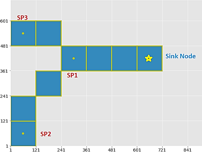
Used Square Sub-Clusters for establishing the communication path between serve points (SP1, SP2, SP3) and the sink node
Fig. 4 
Communication path between serve points and sink node
-
c.
Indexing of deployed WSN nodes in the convex hull for each cluster of the target area:
Index of WSN nodes has been carried out to keep track of the WSN nodes.
-
a.
-
Step 5: Selection of cluster head from the group of previously unselected WSN nodes randomly.
-
Step 6: A modified GA-SAMP-MWPSO algorithm has been applied for the optimization of consumed energy.
-
Step 7: Energy minimization and the number of day-saving have been calculated for the whole WSNs.


To establish an energy-efficient wireless sensor network, three algorithms have been proposed:
-
A.
Modified K-mean clustering algorithm (for selection of sink node for the WSN)
-
B.
The least distance connect first (LDCF) deployment strategy.
-
C.
Modified GA-SAMP-MWPSO algorithm (for energy minimization of efficient WSN)
-
A.
The Modified K-mean Clustering Algorithm:
- Input::
-
: n “serve points”
- Output::
-
Position of k sink nodes
- Step 1: :
-
Selection of K, which is the number of pre-decided “physical clusters”
- Step 2: :
-
Instead of selecting initial k random arbitrary “serve points” as centroids of k clusters, the modified k-mean algorithm uses the median value to select k initial centroids (“serve points”) for the k clusters.
- Step 3: :
-
Calculate the distance between each “serve point” and centroids of the k clusters.
- Step 4: :
-
Assign each serve point to that cluster that has the nearest centroid.
- Step 5: :
-
Recalculate the new mean value of all the positions of the serve points for each cluster.
- Step 6: :
-
Repeat through Step-3 to Step-5 until any of the following stopping criteria is met-
-
The newly formed centroid is not changed.
-
The maximum number of “iterations” is reached. The “iteration” is generally set to a high number and it depends upon the permissible configuration time of the WSN.
-
- Step 7: :
-
Centroids of k clusters denote the position of the k sink nodes. Returns k sink nodes.
-
B.
The Least Distance Connect First (LDCF) deployment strategy:
- Input::
-
A set of Convex Hull with serve points, A set of sink nodes for each Convex Hull
- Output::
-
Locations where WSN can be deployed
- Step 1::
-
For each Convex Hull do the following:
- Step 1.1::
-
For each serve point under the selected Convex Hull find out dy, dx, DTS
dy = No. of hop between serve point and sink node (C) in the Y direction
dx = No. of hop between serve point and sink node (C) in the X direction
DTS = SQRT(dy^2 + dx^2)
- Step 1.2::
-
Sort all the serve points in increasing order of DTS value in a List, LSorted, and set the status of all serve points as U (Unvisited)
- Step 1.3::
-
Select the U status serve point from the list LSorted which has a minimum value and change the status of the selected serve point as T (Temporarily Selected).
- Step 1.4::
-
Find the minimum distance between Temporarily Selected serve point (T) and Selected serve points (SS) and sink node (C).
- Step 1.5::
-
Connect Temporarily Selected serve point (T) with either Selected serve points (SS) or sink node (C) depending on the minimum distance value and store the connection information in LDCF_Path. Change the status of Temporarily Selected serve point (T) as Selected serve point (SS).
- Step 2::
-
Return LDCF_Path, which holds the locations where WSN can be deployed.
- Step 3::
-
End
-
III.
The Modified GA-SAMP-MWPSO Algorithm
In this experiment, the genetic algorithm (GA) has been hybridized with the particle swarm optimization (PSO) algorithm. The GA is such a kind of evolutionary process which takes multiple generations before the global optimal solution is obtained. Not only that, but the population can become stuck in a local optimal value, resulting in premature convergence. During the population process, it is desirable to construct a robust feature and a high convergence rate. To achieve a trade-off between convergence and robustness, the algorithm modified GA has been combined with the modified particle swarm optimization (PSO) algorithm, and the modified GA-SAMP-MWPSO algorithm has been proposed. In this section, first genetic algorithm (GA), then particle swarm optimization (PSO) algorithm and finally modified GA-SAMP-MWPSO algorithm have been discussed.
3.1 The genetic algorithm (GA)
A genetic algorithm is such a technique of optimization [35, 36, 39] in which the bio-inspired mechanism is imitated to solve problems of optimization. The optimization problem can be explained by a single objective or multi-objective function. Reliability optimization problems can be solved using a genetic algorithm [28]. The genetic algorithm used in the research work is inspired by the research work of Sahoo et al. [28].
The modified genetic algorithm can be explained by the below-mentioned operators.
-
(a)
power crossover operator
-
(b)
non-uniform mutation operator
-
(c)
Selection operator
The power crossover operator is explained in Fig. 5. The power crossover is a modern crossover technique where the real part of the problem can be handled very efficiently by this operator.

Flowchart of power crossover
The convergence into local optima is always a challenging problem in any metaheuristic algorithm and to get rid of it one can use an efficient mutation operator like the non-uniform mutation technique. This mutation technique is also used to handle floating points variable used in the mixed-integer optimization problem. The non-uniform mutation technique is explained in Fig. 6.

Flowchart of non-uniform mutation
In Fig. 7, the flowchart of the GA has been explained step by step.

Flowchart of the Genetic algorithm
3.2 The particle swarm optimization (PSO) algorithm
In 1995, Kennedy, Eberhart and Shi first discovered particle swarm optimization (PSO), a unique metaheuristic algorithm inspired by the behavior of real swarm. It is a metaheuristic search algorithm that is built on the notion of "individual experience and social interaction." [28]. In PSO, every object is known as a particle and each particle is a possible solution to the particular problem of optimization. Each particle is provided with a randomized velocity, and all particles pass through the search space. A noble PSO technique, named self-adaptive multi-population-based mean-weighted particle swarm optimization (SAMP-MWPSO), has been proposed. Unlike GA’s crossover and mutation operators, the PSO uses the update operator for updating of “Velocity” vector of each particle for the relocation of the particle. In this research work, the basic PSO algorithm has been modified with the help of the update operator. By varying and controlling the range of weighting coefficient of the velocity vectors (personal and social influence vectors) the decision of the best particle position is determined.
The population is fed into an algorithm named self-adaptive multi-population (SAMP). The SAMP algorithm divides the population into n equal-sized subpopulations and each of these subpopulations is passed to the mean-weighted particle swarm optimization (MWPSO) algorithm. The MWPSO algorithm returns the solution for each subpopulation. During the SAMP algorithm’s selection process, the selection operator determines whether the returned solution from the MWPSO algorithm is acceptable or not by comparing the new solution to the prior solution. The decision or selection process of SAMP leads to finding the best particle’s position. This decision-making factor makes the algorithm flexible for controlling velocity vectors to achieve the best global particle position in the future.
The weighting coefficients, used in the mean-weighted particle swarm optimization (MWPSO) algorithm, are the mean value of different randomly generated weighting coefficients in the allowable range. The mean-weighted approach, in the MWPSO algorithm, promotes the uniformity among divergent random velocity vectors and assists the particle to converge into the uniform global best position.
3.3 Algorithm of self-adaptive multi-population-based mean-weighted particle swarm optimization (SAMP-MWPSO)
- Step 1::
-
Initialize the total populations as PS-MWPSO(t) and termination criterion (i.e., the maximum round of fitness function evaluations, repetition of fitness function value for a certain time, etc.).
- Step 2::
-
Calculate the primary candidate solutions (“initial solution”) using the “fitness function” for the problem.
- Step 3::
-
The entire population is segregated using a new operator called the segregation operator. The whole population is segregated into an equal n number of “subpopulations” depending upon the quality of the solutions.
- Step 4::
-
Each “subpopulation” uses the mean-weighted particle swarm optimization (MWPSO) for modifying the solutions in each subpopulation independently.
- Step 5::
-
In the selection phase, the selection operator is used where the modified solutions are accepted if the new solution is improved than the previous solution.
- Step 6::
-
If any of the following stopping conditions are satisfied, then report the best optimal solution; otherwise, go to Step 3.
-
the maximum round of fitness function evaluations is completed.
-
the repetition of fitness function value for a certain time is noticed
-
- Step 7::
-
End.
3.4 Algorithm of mean-weighted particle swarm optimization (MWPSO)
- Step 1::
-
Initialize the population size and the total number of generations to a finite number.
- Step 2::
-
Set iteration number as t = 0.
- Step 3::
-
Set the “particles” of the current population as P(t).
- Step 4::
-
Compute “fitness functions value” for each particle from P(t).
- Step 5::
-
Search for the “global best particle” (Pg) consuming the “best fitness value.”
- Step 6::
-
Repeat the following steps until the termination criterion is met:
Apply MWPSO update operator for the population P(t). Consider that Pg is the best particle in population P(t).
- Step 6.1::
-
Calculate the “velocity” of each particle using the following equation:
$$V_{i}^{t + 1} = V_{i}^{t} + \alpha \cdot (p_{i}^{t} - p_{i}^{local} ) + \beta \cdot (p_{i}^{t} - p_{i}^{global} )$$where Vit denotes the “velocity” of the ith particle at time instance t and similarly Vit+1 denotes the “velocity” of the ith particle of time instance t+1, i.e., next time instance. α and β are weighting coefficients and pit, pilocal and piglobal give the idea about the current position of the ith particle, the local best position and global best position, respectively. The value of α and β has been calculated separately by taking the mean value of P(t) number of random values within the range 0–2.
- Step 6.2::
-
Obtain a new position in P(t) using the following equation:
$$p_{i}^{t + 1} = p_{i}^{t} + V_{i}^{t + 1}$$where pit and pit+1denote the position of the ith “particle” at time instance t and t + 1, respectively, and Vit+1 denotes the “velocity” of the ith particle at time instance t + 1.
- Step 6.3::
-
Update the position of the best particle in P(t) and find the global best particle.
- Step 7::
-
Validate the termination condition. If the termination condition is not true, then go to Step 6; otherwise, go to Step 8.
- Step 8::
-
Display the value of “position vector” and “fitness value” of the “global best particle.”
- Step 9::
-
End.
3.5 Proposed hybrid algorithm: GA-SAMP-MWPSO
This article describes a “hybrid algorithm,” by merging two metaheuristic algorithms, namely GA and a distinct type of modified PSO, i.e., “self-adaptive multi-population-based mean-weighted particle swarm optimization” (SAMP-MWPSO). The PNW(t) is the initial “population size.” The initial population, PNW(t), is subdivided into two subgroups: The first 50% of the population assigned for GA (PGA(t)), and the rest of the 50% assigned for SAMP-MWPSO (PSS-MWPSO(t)), i.e., PNW(t) = PGA(t) + PS-MWPSO(t).
3.6 Algorithm: GA-SAMP-MWPSO
- Step 1::
-
Set population size [PNW(t)], crossover rate, mutation rate.
- Step 2::
-
Set t = 0.
- Step 3::
-
Initialize simultaneously chromosome and particles of the population for GA and SAMP-MWPSO, respectively.
- Step 4::
-
Calculate the “fitness function value” for each chromosome of PGA(t) and “fitness function value” for every particle of PS-MWPSO(t).
- Step 5::
-
Repeat the following steps until the termination criterion is met:
- 5.1::
-
Increase the time variable, i.e., t = t + 1
- 5.2::
-
Apply GA for population PGA(t).
-
Apply power crossover and non-uniform mutation operators upon PGA(t) to produce a new population PGA(t + 1).
-
Find the current best chromosome (PGAc) from the current population PGA(t) and also maintain the global best chromosome (PGAg)
-
Compare the current best chromosome (PGAc) with the global best chromosome (PGAg) and store the better one in (PGAP).
-
- 5.3::
-
Apply SAMP-MWPSO for PS-MWPSO(t)
-
Self-adaptive multi-population (SAMP) has been used to achieve a higher-quality population.
-
Compute the “velocity vector” of each particle of PS-MWPSO(t)
-
Get the new position of each particle of PS-MWPSO(t).
-
Find the current best particle position (PS−MWPSOc) for the current population PS-MWPSO(t)
-
Modify the current best solution (PS−MWPSOc) using the “mean-weighted” strategy to the basic PSO algorithm to get the global best solution (PS−MWPSOg).
-
- Step 6::
-
Compare the two best global solutions (PGAg, PS−MWPSOg), achieved from steps 5.2 and 5.3, to get the best global solution (Pg).
- Step 7::
-
Validate the termination condition. If the termination condition not true, then go to Step 5; otherwise, go to Step 8.
- Step 8::
-
Display the value of the fitness function, best global solution (Pg).
- Step 9::
-
End.
The block diagram of the GA-SAMP-MWPSO algorithm is given below (Fig. 8).

Block diagram of GA-SAMP-MWPSO algorithm
The stepwise implementation of the Solution Methodology of this research work has been depicted in Figs. 9, 10, 11, 12, and 13. Here the number of physical clusters has been taken as 5. To know the suitable number of the physical cluster the algorithms have been run many times and the elbow method suggests the number of physical clusters in a range of 4–6.

Randomly generated serve points in the target area

Serve points with their centroids (the position of sink nodes denoted by red-colored asterisk *)

Serve points linked with centroids (sink nodes)

Serve points linked with centroids within the convex hull of each physical cluster

Established Communication Network using Square Sub-Clusters
Figures 9, 10, 11, 12 and 13 show the development of WSN step by step. In the same way, the network has also been established for other numbers of physical clusters to observe the various parameters like the number of WSN nodes required, the number of hops required, and so on. Figure 14 collectively shows six established communication networks for 6 different physical clusters.

Six established networks for six different physical clusters (from physical cluster number 1 to physical cluster number 6)
4 Problem formulation
In this paper, the main problem can be segregated into 2 parts: (1) construction of an efficient WSN using the K-mean algorithm and (2) energy minimization of WSN using metaheuristic hybrid algorithm (GA-SAMP-MWPSO). The second problem has been considered a nonlinear problem. The energy consumption was measured and reduced using the following equations [7] during stable data transmission between cluster head (CH) to cluster head (CH) and cluster head (CH) to sink node (SN).
Subject to,
d \(\le\) do, for free space propagation model and d > do for two-ray ground propagation model. where do is the threshold transmission distance.
Where
For two-ray ground propagation model
In this research, the distance between two nodes has been considered in between allowable range, i.e., 50–100 m [17]. The problem can therefore be described as an objective function as follows:
For two-ray ground propagation model
\({E}_{{\rm Amplifier}}^{{\rm CH}-{\rm CH}}\) = Energy needed to maintain an appropriate "signal-to-noise ratio (SNR)" for the transmission of “data packets" between two head-to-head cluster heads for amplification.
\({E}_{{\rm Amplifier}}^{{\rm SN}-{\rm CH}}\) = Energy needed to maintain an appropriate "signal-to-noise ratio (SNR)" for the transmission of “data packets" between two head-to-head sink nodes and cluster heads for amplification.
\({E}_{{\rm Electronic}-{\rm energy}}^{{\rm CH}-{\rm CH}}\) = During the transmission between two neighboring cluster heads, the amount of power deterioration.
\({E}_{{\rm Electronic}-{\rm energy}}^{{\rm SN}-{\rm CH}}\) = During the transmission between adjacent cluster head and sink node, the amount of power deterioration.
Etx = The volume of energy consumed at the time of transfer of “data packets” by each node.
Erx = The amount of energy consumed at the time of receiving of “data packets” by each node.
The following equation is used to calculate the distance between two cluster heads.
where (px1, py1) and (px2, py2) are two head-to-head WSN node coordinates and dxy is the distance determined between two neighboring WSN nodes. The notation dxy and d are the same.
Etr = Amount of energy consumption by a single node for two-ray ground propagation.
For minimization of consumed energy, the proposed GA-SAMP-MWPSO algorithm has been used, and the optimized path has been established as shown in Figs. 9, 10, 11, 12 and 13. The proposed method is tested using the data of Table 1 using the GA-SAMP-MWPSO algorithm and obtained the optimized path for the network for minimizing energy consumption. After forming the network, the longevity of the network has been calculated in terms of day-life.
5 Numerical data analysis
Table 1 has been used to denote the input values used for different parameters in the experiment. The parameters have been used while maintaining the synchronization with the existing literature [17]. In Table 1, different units for energy (Joule and Pico-Joule) were used. Therefore, all measurements were taken in Pico-Joule to ensure uniformity. Now with the help of Eqs. 1–23, the energy consumption by all WSN nodes is calculated.
6 Numerical data representation
Equation No 1 has been used with the help of a hybrid GA-SAMP-MWPSO algorithm to minimize the energy consumed by the optimized WSN. Now the numerical data of results are being represented with the help of tabular format as depicted in Table 2. In Table 1, different units (Joule, Nano-Joule and Pico-Joule) were used, and to maintain uniformity, all calculations have been done in Pico-Joule in Table 2. The number of nodes required to configure WSN and the total number of day-life are two parameters, which have been chosen to compare the value obtained by the experiment in this paper and the existing literature [7].
Considering several parameters related to energy the sustainable days of the whole WSN have been calculated for the different number of physical clusters. The result has been generated by referencing the existing literature [7]. In the existing literature, random deployment and area-wise clustering processes have been used, whereas in the current paper modified K-mean clustering algorithm and LDCF deployment strategy has been used to configure the WSN and GA-SAMP-MWPSO hybrid algorithm has been proposed to minimize the consumed energy.
The experimental findings have been tallied with the research literature [7], GA algorithm and PSO algorithms, and it has been found that the proposed methodology yields 15.5544456 day-life of the network where other approaches give 6.333777 day-life, 8.39 day-life and 7.49 day-life of the network, respectively. Furthermore, the suggested technique requires just 23 WSN nodes to configure the network, whereas the existing literature's algorithm requires 49 WSN nodes, the GA algorithm requires 65 WSN nodes, and PSO requires 58 WSN nodes. The proposed algorithm produces a satisfactory result.
7 Result analysis
When this research work is compared with other literature [7], then it is found that our experiments have yielded better results than other papers.
7.1 Applying random deployment strategy and area-wise clustering process
By applying random deployment strategy and area-wise clustering process, the calculations of the energy saved are shown in Table 2. Considering the initial energy as 1 Joule per node, the day-life has been calculated
where Es = Energy consumed and 1 day = 86,400 s.
Putting the value of ES as 1,756,090,368, we get 6.333777229 day-life for the existing literature [7, 8].
So, this network can sustain up to 6.333777229 days, i.e., 6–7 days.
7.2 Applying least distance connect first (LDCF) deployment strategy and K-mean clustering process
By applying least distance connect first (LDCF) deployment strategy and K-mean clustering process, the calculations of the energy saved are shown in Table 2. Considering the initial energy as 1 Joule per node, the day-life has been calculated
where Es = Energy consumed and 1 day = 86,400 s.
Putting the value of ES as 1,523,432,979.25, we get 15.5544456 day-life in this paper.
So, this network can sustain up to 15.5544456 days, i.e., 15–16 days.
7.3 Statistical analysis
The target area has been physically clustered, and within the physical cluster, the WSN has been configured. The number of physical clusters has been varied from 1 to 7. It means the same target area has been clustered once, twice, thrice, four times, five times, six times and seven times, and the following parameters have been monitored.
-
a.
Total no. of square sub-clusters needed to configure the network
-
b.
Total no. of hops needed to accomplish communication path
-
c.
The total coverage area of the configured network
To get sufficient information on the above-mentioned parameters, for each physical cluster, the proposed algorithm has been executed 50 times. After running the algorithm 50 times for each cluster, the acquired information on the above-mentioned parameters has been summarized in Table 3. Table 3 gives the following information.
-
Minimum and maximum number of square sub-clusters needed to configure the network
-
Minimum and maximum number of hops needed to accomplish communication path
-
Minimum and maximum coverage area of the configure the network
According to the first row of Table3, for physical cluster number1, a minimum of 117 hops and a maximum of 178 hops are required to configure the network. On average, 146 hops are needed to configure the network. In the same way, it can be noticed that for physical cluster number1, a minimum of 23 Square Sub-Clusters and a maximum of 34 square sub-clusters are required to configure the network. On average, 30 square sub-clusters are needed to configure the network. For physical cluster number1, the minimum and maximum network coverage areas are 14,463 m2 and 21,850 m2, respectively.
Each row of Table 3 gives the information about the number of hops, the number of square sub-cluster, coverage area in maximum, minimum, mean and median format. Each row of Table 4 tries to depict more information (in a frequency diagram format) on the number of hops, number of square sub-cluster.
Rows 1–7 of Table 4 represent the frequency diagram for physical cluster numbers 1–7, respectively. The frequency diagram of the first row and first column of Table 4 shows that for physical cluster number 1, the network has been configured only 1 time (out of 50 runs) utilizing 23 square sub-clusters. Similarly, it can be noticed that out of 50 runs 13 times network has been configured utilizing 26–29 square sub-clusters. Out of 50 runs, 27 times network has been configured utilizing 30–32 square sub-clusters. Out of 50 runs, 9 times network has been configured utilizing 33–34 square sub-clusters. So, it can be said that 1, 13, 27, 9 times network has been configured utilizing 23–25, 26–29, 30–32, 33–34 square sub-clusters, respectively.
The frequency diagram of the first row and second column of Table 4 shows that for physical cluster number 1, the network has been configured only 2 times (out of 50 runs) utilizing 110–124 hops. Similarly, it can be noticed that out of 50 runs 7 times network has been configured utilizing 125–138 hops. Out of 50 runs, 28 times network has been configured utilizing 139–152 hops. Out of 50 runs, 10 times network has been configured utilizing 153–166 hops. Out of 50 runs, 3 times network has been configured utilizing 167–180 hops. So, it can be said that 2, 7, 28, 10, 3 times network has been configured utilizing 110–124,125–138, 139–152, 153–166 and 167–180 hops, respectively.
In the above section, the observation of the number of required square sub-cluster and the number of required hops for the physical cluster number 1 has been illustrated. The reader can easily understand the other observation from physical clusters no 2 to 7 in the same way.
8 Conclusion
The main goal of this paper is to construct an efficient wireless sensor network. The efficiency of the network can be expressed in terms of total day-life durability. The durability of the network depends on limited battery-powered stored energy. If the consumed energy is minimized, then the durability of the network is maximized. As a result, the network remains operational for a longer time. So, the efficiency of the network directly depends on the minimization technique of the consumed energy. From the existing literature, it is revealed that very little effort has been made to address the issue of developing energy-efficient WSNs utilizing hybrid algorithms with machine learning algorithms. In this research work, a modified K-mean algorithm from the machine learning domain has been used to select the suitable position of the sink node within the cluster. The position of the sink node helps to minimize the cumulative communication distance from the sink node to every serve point. This minimization of the cumulative communication distance helps to minimize the consumed energy of the whole WSN. The LDCF deployment strategy also helps to minimize the consumed energy of the whole WSN. After configuring the WSN by using a modified K-mean algorithm and LDCF deployment strategy, a modified metaheuristic algorithm (GA-SAMP-MWPSO) has been used to find the optimized energy consumption for the network. The result has been compared with the existing literature and it has been noted that the proposed technique yields 15.5544456 day-life of the network where the existing literature’s approach gives 6.333777 day-life of the network. The proposed algorithm delivers a better outcome theoretically. The best result set has been chosen among all the obtained results considering various parameters (equivalent distribution, the number of iterations, maximum energy consumption) within the permissible range. The Fuzzy logic can be used in the future to include uncertainty into experimental results, making the scenario more realistic. The current study has solely used the two-ray propagation model. In the future, the free space propagation model can be used to improve the research work.
Availability of data and material
Authors have the required data and supporting materials.
References
Abdulla AE, Nishiyama H, Yang J, Ansari N, Kato N (2012) HYMN: A novel hybrid multi-hop routing algorithm to improve the longevity of WSNs. IEEE Trans Wirel Commun 11(7):2531–2541
Alghamdi TA (2020) Energy efficient protocol in wireless sensor network: optimized cluster head selection model. Telecommun Syst 74:1–15
Alsheikh MA, Lin S, Niyato D, Tan HP (2014) Machine learning in wireless sensor networks: algorithms, strategies, and applications. IEEE Commun Surv Tutor 16(4):1996–2018
Arora S, Singh S (2017) Node localization in wireless sensor networks using butterfly optimization algorithm. Arab J Sci Eng 42(8):3325–3335
Ayadi H, Zouinkhi A, Boussaid B, Abdelkrim MN (2015) Machine learning methods: outlier detection in WSN. In: 2015 16th International Conference on Sciences and Techniques of Automatic Control and Computer Engineering (STA). IEEE, pp 722–727
Aznoli F, Navimipour NJ (2017) Deployment strategies in the wireless sensor networks: systematic literature review, classification, and current trends. Wirel Pers Commun 95(2):819–846
Banerjee A, Das V, Biswas A, Chattopadhyay S, Biswas U (2021) Development of energy efficient and optimized coverage area network configuration to achieve reliable WSN network using meta-heuristic approaches. Int J Appl Metaheuristic Comput 12(3):1–27
Banerjee A, Das V, Mitra A, Chattopadhyay S, Biswas U (2021b) A power optimization technique for wsn with the help of hybrid meta-heuristic algorithm targeting fog networks. In: Intelligent and cloud computing. Springer, Singapore, pp 105–123
Bangyal WH, Ahmed J, Rauf HT (2020) A modified bat algorithm with torus walk for solving global optimisation problems. Int J Bio-Inspired Computa 15(1):1–13
El Mezouary R, Choukri A, Kobbane A, El Koutbi M (2015) An energy-aware clustering approach based on the k-means method for wireless sensor networks. In: International symposium on ubiquitous networking. Springer, Singapore, pp 325–337
Ghate VV, Vijayakumar V (2018) Machine learning for data aggregation in WSN: a survey. Int J Pure Appl Math 118(24):1–12
Jain SR, Thakur NV (2015) Overview of cluster based routing protocols in static and mobile wireless sensor networks. In: Information systems design and intelligent applications. Springer, New Delhi, pp 619–626
Jang WS, Healy WM (2010) Wireless sensor network performance metrics for building applications. Energy Build 42(6):862–868
Jayarajan J, Prabhu S (2016) Comparison of energy minimization techniques in wireless sensor networks. In: 2016 International Conference on Global Trends in Signal Processing, Information Computing, and Communication (ICGTSPICC). IEEE, pp 593–598
Khattak A, Asghar MZ, Ishaq Z, Bangyal WH, Hameed IA (2021) Enhanced concept-level sentiment analysissystem with expanded ontological relations for efficient classification of user reviews. Egypt Inform J 22:455–471
Kumar DP, Amgoth T, Annavarapu CSR (2019) Machine learning algorithms for wireless sensor networks: a survey. Inf Fus 49:1–25
Lande SB, Kawale SZ (2016) Energy Efficient routing protocol for wireless sensor networks. In: 2016 8th International Conference on Computational Intelligence and Communication Networks (CICN). IEEE, pp 77–81
Liu S, Yu M, Li M, Xu Q (2019) The research of virtual face based on deep convolutional generative adversarial networks using tensorflow. Phys A 521:667–680
Marutho, D., Handaka, S. H., & Wijaya, E. (2018). The determination of cluster number at k-mean using elbow method and purity evaluation on headline news. In: 2018 international seminar on application for technology of information and communication. IEEE, pp 533–538
Midya S, Roy A, Majumder K, Phadikar S (2018) Multi-objective optimization technique for resource allocation and task scheduling in vehicular cloud architecture: a hybrid adaptive nature inspired approach. J Netw Comput Appl 103:58–84
Mydhili SK, Periyanayagi S, Baskar S, Shakeel PM, Hariharan PR (2019) Machine learning-based multi-scale parallel K-means++ clustering for cloud-assisted internet of things. Peer-to-Peer Netw Appl 13:1–13
Ouchitachen H, Hair A, Idrissi N (2017) Improved multi-objective weighted clustering algorithm in wireless sensor network. Egypt Inform J 18(1):45–54
Pandey OJ, Hegde RM (2018) Low-latency and energy-balanced data transmission over cognitive small world WSN. IEEE Trans Veh Technol 67(8):7719–7733
Rahman AU, Alharby A, Hasbullah H, Almuzaini K (2016) Corona based deployment strategies in wireless sensor network: a survey. J Netw Comput Appl 64:176–193
Randhawa S, Jain S (2019) MLBC: Multi-objective load balancing clustering technique in wireless sensor networks. Appl Soft Comput 74:66–89
Rao PS, Jana PK, Banka H (2017) A particle swarm optimization based energy efficient cluster head selection algorithm for wireless sensor networks. Wireless Netw 23(7):2005–2020
Rhim H, Tamine K, Abassi R, Sauveron D, Guemara S (2018) A multi-hop graph-based approach for an energy-efficient routing protocol in wireless sensor networks. HCIS 8(1):1–21
Sahoo L, Banerjee A, Bhunia AK, Chattopadhyay S (2014) An efficient GA–PSO approach for solving mixed-integer nonlinear programming problem in reliability optimization. Swarm Evol Comput 19:43–51
Shankar T, Karthikeyan A, Sivasankar P, Rajesh A (2017) A hybrid approach for optimal cluster head selection in WSN using leach and monkey search algorithms. J Eng Sci Technol 12(2):506–517
Sharma D, Arora B (2021) Hybridization of energy-efficient clustering and multi-heuristic strategies to increase lifetime of network—a review. Innov Inf Commun Technol (IICT-2020) 2021:387–392
Shukla A, Tripathi S (2020) An effective relay node selection technique for energy efficient wsn-assisted iot. Wirel Pers Commun 112(4):2611–2641
Solaiman B (2016) Energy optimization in wireless sensor networks using a hybrid k-means pso clustering algorithm. Turk J Electr Eng Comput Sci 24(4):2679–2695
Vijayalakshmi K, Anandan P (2019) A multi objective Tabu particle swarm optimization for effective cluster head selection in WSN. Clust Comput 22(5):12275–12282
Wang F, Wang C, Wang Z, Zhang XY (2015) A hybrid algorithm of GA+ simplex method in the WSN localization. Int J Distrib Sensor Netw 11(7):731894
Xu Q (2013) A novel machine learning strategy based on two-dimensional numerical models in financial engineering. Math Probl Eng 2013:1–6
Xu Q, Wu J, Chen Q (2014) A novel mobile personalized recommended method based on money flow model for stock exchange. Math Probl Eng 2014:1–9
Xu Q, Huang G, Yu M, Guo Y (2020) Fall prediction based on key points of human bones. Phys A Stat Mech Appl 540:123205
Xu Q, Wang Z, Wang F, Gong Y (2019) Multi-feature fusion CNNs for Drosophila embryo of interest detection. Phys A Stat Mech Appl 531:121808
Xu Q, Wang F, Gong Y, Wang Z, Zeng K, Li Q, Luo X (2019) A novel edge-oriented framework for saliency detection enhancement. Image Vis Comput 87:1–12
Yuan X, Elhoseny M, El-Minir HK, Riad AM (2017) A genetic algorithm-based, dynamic clustering method towards improved WSN longevity. J Netw Syst Manage 25(1):21–46
Acknowledgements
We would like to thank the officials of the “Journal of Supercomputing” for giving us the opportunity of submitting this manuscript.
Funding
This study was not funded by any organization.
Author information
Authors and Affiliations
Contributions
Every author has contributed significantly.
Corresponding author
Ethics declarations
Competing interests
The authors declare that they have no competing interests.
Additional information
Publisher's Note
Springer Nature remains neutral with regard to jurisdictional claims in published maps and institutional affiliations.
Rights and permissions
About this article

Cite this article
Banerjee, A., De, S.K., Majumder, K. et al. Construction of energy minimized WSN using GA-SAMP-MWPSO and K-mean clustering algorithm with LDCF deployment strategy. J Supercomput 78, 11015–11050 (2022). https://doi.org/10.1007/s11227-021-04265-7
Accepted:
Published:
Issue Date:
DOI: https://doi.org/10.1007/s11227-021-04265-7