
Abstract
In the field of welding process control, on-line monitoring of welding quality based on multi-sensor information fusion has attracted more attention. In order to recognize the penetration state of the Keyhole mode Tungsten Inert Gas welded joint in real time, an acoustic and visual sensing system was established in this paper. The acoustic and visual features that characterize the penetration state of the welded joints in 34 dimensions were extracted and the variation of the acoustic signal and the keyhole geometry were analyzed. In addition, the weighted scoring criterion based on the Fisher distance and the maximum information coefficient (Fisher–MIC) and Support Vector Machine (SVM) model based on cross-validation (CV) are designed as the feature selection method. The feature selection method can evaluate the penetration recognition accuracy of different feature subsets. The experiment results show that the maximum recognition accuracy was 97.1655%, which was performed by the 10-dimension optimal feature subset and the CV–SVM model with particle swarm optimization (PSO–CV–SVM). It is proved that the selected acoustic and visual features can well characterize the penetration state of the welded joints, and the feature selection method and PSO–CV–SVM model have superior performance.
1 Introduction
K-TIG welding is a new deep penetration welding method which can form a keyhole. The keyhole achieves dynamic equilibrium under large arc pressure that is formed by high current (300–1000 A), liquid metal static pressure and surface tension in the keyhole. K-TIG welding can weld plates of 3–16 mm in a single pass with double-sided forming. However, because of the effect of the thermal accumulation and the errors of machining and assembly, it is difficult to ensure good penetration of all welded joints in an actual welding environment. Therefore, the quality of the welded joints can be better guaranteed only when the penetration state of the welded joints was recognized in real time.
In order to monitor welding quality in real time, the primary task is to obtain features characterizing the welding quality. Therefore, various sensors are used to capture welding process signals, such as voltage sensors [1], vision sensors [2,3,4], spectral sensors [5, 6], acoustic sensors [7,8,9], etc. For the above mentioned sensors, the application of acoustic sensing or visual sensing for penetration control and defect detection has attracted wide attention. During K-TIG welding, the arc acoustic signal has advantages of good real-time performance, which can reflect the internal changes of the arc and molten pool, but it is susceptible to electromagnetic interference and the influence of the workpiece deformation. It is especially suitable for real-time monitoring of welding quality. Although the visual sensor can directly reflect the geometry of the keyhole, it is susceptible to arc, electromagnetic interference. Tarn et al. has proved that acoustic and visual signals are complementary and the combination of them has a great significance to realize intelligent welding [10]. But so far, studies on K-TIG welding have only been limited to the welding process and keyhole stability [11,12,13], and there is no study on the recognition of weld penetration. The strong arc light and electromagnetic interference during K-TIG welding bring great challenges to extracting penetration features. Therefore, recognizing weld penetration during K-TIG welding is worthy of further study.
Considering that the welding process is time-varying and single-sensing mode can only obtain local information, acoustic and visual information were fused in this paper to obtain intrinsic feature subsets that characterize the penetration state, thereby improving the reliability of the sensing system and penetration state recognition accuracy. At present, multi-sensor information fusion is widely used in robotics [14], intelligent transportation [15], factory monitoring [16] and other fields. In the field of welding quality control, Chen et al. [17,18,19] used fusion theories of D-S evidence theory and weighted average coefficient theory to fuse various sensing information in pulsed TIG welding, realizing penetration identification of joints. Lee et al. [20]. integrated various information in ultrasonic welding to characterize the quality of welded joints. However, most studies in this field have strong subjectivity in feature selection, and have not investigated the characterization and recognition capabilities of different feature types and quantities for penetration states. Therefore, the feature selection theory in pattern recognition was introduced to study the influence of the dimension of feature subsets on the accuracy of penetration recognition, and as low dimensions of feature subsets as possible were used to reasonably characterize the penetration state of welded joints.
In this paper, acoustic and visual sensing were combined to construct a practical dual sensing system. The acoustic and visual features were extracted from multiple perspectives and the variations in the acoustic and visual signal during K-TIG welding were analyzed. Feature selection method was used to find the optimal feature subset and reduce the feature redundancy. The PSO–CV–SVM model was proposed to automatically recognize the penetration state of welded joints and then the highest accuracy was obtained on the optimal feature subset. The results show that the penetration state of welded joints can be well characterized and recognized by using feature selection and penetration modeling. In addition, a higher recognition accuracy can be obtained by fusing multiple sensing information than that of single sensing information.
2 Experimental Setup
As shown in Fig. 1, the experimental system consists of four modules: a robot module, a K-TIG welding module, a control module and a sensing module. The sensing module is mainly composed of a CCD and a microphone. The CCD camera is equipped with a narrow-band pass filter whose central wavelength is 810 nm, bandwidth is 40 nm, and transparency is about 80%.The observation is toward the rear of the weld pool, and the viewing angle is set to 35°. The distance from the center of the camera lens to the object plane is around 200 mm. The microphone is omnidirectional capacitance MP201 microphone, which has the frequency response from 20 Hz to 20 kHz. It was fixed with the angle of 80° over the backside of the workpiece, 100 mm away from the center of the back weld. Meanwhile, the NC1004 signal conditioner is used as an auxiliary equipment. Acoustic and visual signal acquisition is triggered synchronously by an industrial control unit, and the acquisition frequency is 42 kHz and 14 f/s, respectively.

Dual sensing system for K-TIG welding
Workpieces of 304 stainless steel with dimensions of 300 × 200 × 11.8 mm were used in the experiments. The butt joint gap was 1 mm without a groove, as shown in Fig. 2. A large number of experiments were carried out to obtain different penetration states by changing welding current generated by a welding power source whose output current is continuous DC. According to the width of the backside bead of the workpiece, the penetration state of welded joints can be divided into three categories, namely, partial penetration (width < 1 mm), full penetration (1 mm ≤ width <2.5 mm) and excessive penetration (width ≥2.5 mm), as shown in Fig. 3. It was found that the partial penetration occurred as the welding current was 500A. When the welding current increased to 580A, the molten pool was easy to collapse, which led to excessive penetration. Therefore, the range of welding current selected in this investigation was between 500 and 580 A. Experimental parameters are shown in Table 1.

Schematic diagram of the weld groove

Schematic diagram of penetration states. a Partial penetration. b Full penetration. c Excessive penetration
3 Feature Extraction and Analysis
As depicted in Fig. 4, 28 acoustic features and 3 visual features were extracted respectively. Considering that the time sequence and heat accumulation have effects on the welding process, the first-order difference of the three visual features were seen as new features and a 34-dimension feature set was finally obtained.

Flow chart of feature extraction
3.1 Acoustic Feature Extraction
3.1.1 Preprocessing of Acoustic Signals
The acoustic signal is a non-stationary random signal. Every 3000 sampling points of the acoustic sequence were recorded as one frame to meet the requirement of processing accuracy, and the corresponding analysis duration and weld length were 0.0714 s and 0.2500 mm, respectively. The sample points corresponding to the acoustic signals, which changed drastically during the arcing and extinction phases, were discarded. The effective acoustic signal was obtained as shown in Fig. 5a. It can be seen that the amplitude of the sound increases as the welding current increases. For a better analysis of the acoustic signal frequency, the DC offset was removed according to Eq. (1). Figure 5b shows the signal after removing the DC offset.

Acoustic signal before and after removing DC offset. a The effective acoustic signal. b Acoustic signal after removing DC offset
where \(x_{i}\) and \(x_{i}^{'}\) are the values of each frame before and after the removing DC offset, n is the total number of data in each penetration state.
In order to filter out noises, FFT spectrum was firstly calculated with the results shown in Fig. 6. According to statistics results, the first 95% of the total amplitude is within 0–18 kHz. And several obvious spectral lines are included in the spectrum, which proves that there is a definite periodic oscillation signal in the acoustic signals during K-TIG welding. Although the spectrum of the acoustic signals contains a large number of components with small amplitude, which may be related to the welding equipment, shielding gas flow and environmental noises, it has no effect on the characteristic analysis of the arc acoustic signals [21, 22].

FFT spectrum of the acoustic signal
According to the above analysis, a method combining sliding median filtering of 1 × 5 rectangular window and Butterworth low-pass filtering with a stop frequency of 18 kHz is designed. The acoustic signal after denoising is shown in Fig. 7. Compared with Fig. 5b, it can be seen obviously that some high-frequency mutation points have been filtered out by using this method.

Acoustic signal after denoising
3.1.2 Feature Extraction
In order to overcome the subjectivity and blindness during the process of feature extraction, a variety of possible related features were extracted. Some features in the time domain were extracted, such as the mean, root mean square (RMS), variance and kurtosis. They were selected to characterize the mean amplitude, effective value, intensity of change and distribution characteristics, respectively. And the analysis of frequency spectrum for acoustic signal in different penetration states was carried out. Figure 8 shows the FFT spectrum and partially amplified spectrum within 0–2 kHz for the acoustic signals. It can be seen that under different penetration states, the low-frequency components gradually change from a multi-peak pattern to a single peak pattern. However, the characteristic frequency of high-frequency components gradually increases. This is mainly because the energy is concentrated on high frequencies when the penetration state changes. In addition, the characteristic frequencies with obvious spectral line family are mostly concentrated in 0–2 kHz, 2–4 kHz and 6–8 kHz. Therefore, FFT amplitude spectrum was divided into 6 segments: 0–2 kHz, 2–4 kHz, 4–6 kHz, 6–8 kHz, 8–14 kHz and 14–20 kHz. And then the mean, RMS, variance and kurtosis were calculated in each segment. Figure 9 shows RMS corresponding to different frequency bands, which indicates that different frequency bands have different changing trends for the same penetration state. The first four segments are sensitive to changes in the penetration state. And only frequency bands within 2–4 kHz and 4–6 kHz corresponding to RMS can be used to clearly distinguish three kinds of penetration state.

FFT spectrums corresponding to different penetration states. a Partial penetration. b Full penetration. c Excessive penetration

RMS corresponding to different frequency bands with the two dotted green vertical lines denoting current transition points (Color figure online)
3.2 Image-Based Keyhole Feature Extraction
In the acquired images, the keyhole is approximately oval in shape, and the gray values of the pixels directly below the keyhole are very similar to those of the keyhole, which is caused by the tail flame of plasma gas. In order to comprehensively characterize the variations of the keyhole, the area of the keyhole, eccentricity and exit deviation [23] were extracted to characterize the size, shape and location of the keyhole. A camera calibration experiment was performed to obtain the mapping relation between image pixels and real distance, where Kx = 0.0200 mm/pixel and Ky = 0.0385 mm/pixel.
According to the characteristics of the gray image of the keyhole, a 5 × 5 disc-shaped structural element was used to perform the morphological erosion in the fixed ROI. And then multi-level threshold segmentation method was adopted to obtain the binary image of the keyhole. The method was implemented by Eq. (2) and Eq. (3),
where f(x, y) denotes the gray value of the original image, h(x, y) and g(x, y) denote the gray value at the image coordinate (x, y) after two segmentation, \(T_{1} = 240\), \(T_{2}\) is the threshold calculated by the Otsu method for h(x, y).
The Otsu method can be expressed as Eq. (4),
where \(T\) is the threshold of segmentation, \(\omega_{0} \left( T \right)\) and \(\omega_{1} \left( T \right)\) are the ratio of the target pixels and background pixels to the number of pixels whose gray value is greater than 0 in h(x, y); \(u_{0} \left( T \right)\) and \(\mu_{1} \left( T \right)\) are the average gray values of the target pixels and the background pixels, respectively, \(\upmu\) is the average value of pixels whose gray value is greater than 0 in h(x, y).
The optimal threshold \(T_{2}\) is obtained by the maximum \(\sigma_{B}^{2} \left( T \right)\) and the segmented image is shown in Fig. 10b. After the above steps, the keyhole image is accurately segmented from the background. Finally, the complete keyhole edge was extracted by fitting an ellipse to the binary image using a least-squares method, and three features were extracted in the last step, such as area, eccentricity and deviation.

The procedure of the keyhole image processing. a ROI. b Multi-level threshold segmentation. c Ellipse fitting (Color figure online)
The procedure of keyhole image processing and keyhole images under different currents are shown in Figs. 10 and 11, respectively. In Figs. 10c and 11, the red asterisks denote the boundary points of keyhole images obtained by scanning binary images every 15 lines, and the green curves denote the fitted ellipse whose centers are denoted as blue asterisks. At the same time, in Fig. 11, the arrow with the label of v indicates the welding direction.

Keyhole images under different currents. a 500A. b 540A. c 580A (Color figure online)
3.3 Analysis on Variation of the Acoustic and Visual Signals
In Fig. 12, the two dotted green vertical lines denote current transition points. It can be seen that the two kinds of signal have the same trend, but the former changes more sharply with the different penetration and is more sensitive to current. At the same time, the keyhole area can better distinguish partial penetration and full penetration, but it is not suitable to distinguish the first two classes from the third one because of its instability during excessive penetration, while the acoustic signal is just the opposite. It indicates heterogeneous signal combinations from different sensors have some complementarity to better distinguish all penetration states. In order to further analyze the similarity between the keyhole area and the acoustic signal, cross-correlation analysis was performed on the acoustic signal, the keyhole area and the differential signals of the two, and four cross-correlation coefficients were obtained. For each coefficient, the cross-correlation coefficient between the keyhole area and acoustic signal is the largest. As shown in Fig. 13, the maximum value of 0.8581 appears at the zero delay, indicating that the two signals are almost synchronous and changing in the same direction.

Keyhole area and acoustic signal

Cross-correlation analysis
As the welding current increases, the area of the keyhole increases, and the amplitude of the acoustic signal increases synchronously. The mechanism of this phenomenon may be qualitatively analyzed by Eq. (5),
where I is the amplitude of the acoustic signal, p is the arc plasma pressure, ρ is the air density, v is the velocity of the acoustic signal in the air.
As the current increases, the amount of heat input into the keyhole increases, leading keyhole area becoming larger [24], which indirectly increases the volume of metal vapor and plasma jetting into the air from the backside of the workpiece. Then we expect the I to increase as well when the other variables are substantially unchanged.
Studying the frequency distribution of the acoustic signal as shown in Fig. 8, within 0–2 kHz, it seems that there are little changes in partial penetration and full penetration, but the spectral characteristics change from multi-peak to single-peak and the maximum amplitude of the characteristic frequency becomes significantly larger when excessive penetration. And within 2–20 kHz, there are not so much frequency shift or magnitude change of characteristic frequency.
4 Feature Selection and Penetration Recognition
In pattern recognition, high-dimension features can easily cause “dimensional disasters”. And most scholars qualitatively analyze the correspondence between features and penetration states, subjectively selecting some relevant features or fusing all extracted features, which will inevitably reduce the versatility and robustness of the algorithm [25, 26]. Therefore, the incorporated filtering and packaging methods were used to find the optimal feature subset in order to recognize the penetration state. The normalized Fisher distance and MIC of the 34-dimension feature were calculated, and the weighted scores with corresponding weights assigned to 0.8 and 0.2 were obtained and sorted from high to low. Based on the CV–SVM model, the correspondence between different feature subsets and recognition accuracy was obtained. Finally, using the optimal feature subset as the input of PSO–CV–SVM model, penetration recognition and model validation were performed. And the process of feature selection was shown in Fig. 14.

Flow chart of feature selection
4.1 Feature Selection Based on Weighted Scoring Criteria and CV–SVM
Fisher distance is a feature subset evaluation criterion that is universally used. The maximum and normalized Fisher distance of 3 Fisher distances for each feature was taken as the Fisher distance. Apart from the divisibility of samples, the relevance of features and categories are also considered. Traditionally, mutual information is used to evaluate correlation, and its definition is shown in Eq. (6),
where x and y are two related random variables, p(x, y), p(x) and p(y) are the corresponding probabilities, respectively.
However, this calculation has higher time complexity and lower accuracy. Therefore, MIC was introduced as an improved method [27], the definition of which is shown in Eq. (7),
where I(X; Y) is obtained by dividing the entire X and Y axis into sections as the approximate value of I(x; y), B is the maximum number of sections in the X and Y axis.
The ranking results of the top 15 features are shown in Table 2. It can be seen that different features have different sensitivity to the change of the penetration state. The features with high scores mainly focus on the features of the acoustic signal in time domain and the features within 0–2 kHz and 8–14 kHz in the frequency domain. Compared with mean amplitude, RMS and variance, kurtosis is not suitable for characterizing the penetration states of the welded joints. Because it mainly describes the distribution characteristics of the acoustic waveform. It is known that the acoustic waveform changes a lot during the welding process, especially at the time of partial penetration and excessive penetration, so kurtosis fails to characterize the real welding process. Therefore, it is required that the selected features are not only sensitive to the change of the penetration state, but also have consistent stability.
After feature sorting, it was still impossible to evaluate the relationship between the dimension of feature subsets and the accuracy of penetration recognition. Therefore, the multiple features were fused for further subset selection based on the CV–SVM model. The search strategy of “Sequential Forward Selection” was adopted, namely, new features were selected one by one from the sorted features to form a new feature subset. As shown in Fig. 15, the mean accuracy of 10-fold cross-validation was used as the evaluation criterion to analyze the sensitivity of different feature subsets. From the figure, with the increase of the dimension of feature subset, on the one hand, the recognition accuracy may decrease due to the correlation between features; on the other hand, the processing time and feature redundancy are increased. When the dimension is 10, the highest recognition accuracy is 89.7959% without optimized. And when the dimension is 7–14, more than 85% of the recognition accuracy can be obtained. Therefore, the dimension of the feature subset is not as high as possible, but there is an ideal dimension window, i.e., 7–14. At the same time, it can be concluded that higher classification accuracy can be obtained by fusing two kinds of sensing information.

Recognition accuracy at different subset dimensions
4.2 Recognition of Penetration
In order to accurately recognize the penetration state of welded joints, a recognition model based on PSO–CV–SVM was established by applying acoustic and visual features. There are four main steps:
- 1.
Acquiring training and testing dataset
Referring to Fig. 15, the top 10 features in Table 2 was finally selected as inputs. Experiments were sequentially performed on the same workpiece according to the parameters of Table 1, and the bead appearances of the welds were obtained as shown in Fig. 16. During the whole welding process, the penetration state is from partial penetration to full penetration and then to excessive penetration. At the beginning of welding, the current is small, the back weld width is small and the penetration state is partial penetration and discontinuous. As the welding current increases, the back weld width increases slowly and the middle section of the weld is fully penetrated. However, at the end of the welding, due to the excessive current, the back weld width increases significantly and the weld is excessively penetrated. A total of 980 valid samples were extracted, and the numbers of partial penetration, full penetration, and excessive penetration samples were 294, 392 and 294, respectively, which were donated by category labels “1”, “2” and “3”. Each cycle of ten cycles, 882 samples in the whole sample set were randomly selected as training samples, and the remaining 98 were used as testing samples.

Bead appearances of the welds. a–c the front side, d–f the back side
- 2.
Preprocessing training and testing dataset
Since the input and output have different dimensions and ranges, normalization processing is required. All features are linearly normalized to [0, 1] according to Eq. (8),
where \(x_{origin} {\text{and }}x_{new}\) are the features before and after normalization, \(x_{max} {\text{and }}x_{min}\) are the maximum and minimum values of each feature.
- 3.
Model parameters selection and optimization
As an intelligent modeling method, SVM model shows many advantages in finding globally optimal solutions for problems with small training samples, high dimension and non-linearity. For a multiclass problem, the kernel function is usually used to map data into high-dimension space. The radial basis function (RBF), which is flexible and widely used, was employed here as the kernel function, and its expression is shown in Eq. (9),
where x is any point in space, \(x_{c}\) is the center of the kernel function, σ is the amplitude of Gaussian function.
For RBF kernel, c and σ are two most important parameters, which determine the performance of the SVM model. In this paper, PSO was used to quickly select c and σ, and 10-fold cross-validation method was used to then obtain penetration accuracy with more robustness. The accuracy obtained by CV–SVM in the training set was used as the fitness function value of PSO, the population and individual speeds in the particle swarm were continuously updated. The parameters of PSO were set as shown in Table 3. And then, the value of c and σ with the highest test accuracy on the respective subsets were determined. Finally, the PSO–CV–SVM model was built by using the optimal parameters.
- 4.
Recognition results
The test accuracy of CV–SVM model was 89.7959%. After PSO iterative optimization, the accuracy of 97.1655% was obtained, and the parameters of PSO–CV–SVM model were: c = 4.7682, σ = 1.4134. The testing and PSO results are shown in Figs. 17 and 18, respectively. The results show that the model can effectively recognize and classify the penetration state of the welded joints. At the same time, the classification accuracy of partial penetration and full penetration is lower, mainly because some features in the state of partial penetration and full penetration overlap largely during state transition.

Testing results

PSO results
4.3 Model Verification
Using the dataset obtained in Sect. 4.2.1, principal component analysis (PCA) and CV–SVM model were respectively compared with the methods proposed in this paper, respectively, verifying the effectiveness of Fisher–MIC and PSO method.
- 1.
PCA was performed on the 34-dimension feature set, and the accumulated contribution rate of the first nine principal components reaches 99.9998%. The feature dimension selected by the Fisher–MIC method was 7–14. The comparison between PCA and Fisher–MIC was shown in Table 4. It is obvious that the Fisher–MIC method can achieve better recognition performance, mainly because PCA is unsupervised and can obtain better results only in large samples.
Table 4 Comparison of two feature selection methods - 2.
As shown in Fig. 19 and Table 5, compared with the CV–SVM model, the recognition accuracy and stability of PSO–CV–SVM model are better, indicating that PSO has a significant optimization effect on the SVM model. The main reason is that optimized parameters of PSO–CV–SVM model can better control the trade-off between accuracy and generalization ability than that of default parameters.
Fig. 19 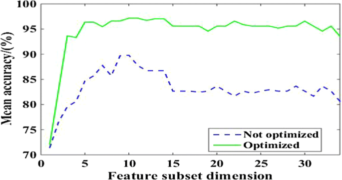
Comparison of accuracy before and after PSO
Table 5 Comparison of two models

5 Conclusions
-
1.
An acoustic and visual sensing system was established to acquire acoustic and visual information, and then the 34-dimension feature characterizing the penetration state of welded joints were designed by fusing the acoustic and visual information.
-
2.
Through experiments and analysis, changes in the penetration state of welded joints during K-TIG welding lead to regular variations of features that characterize acoustic and visual signals. In particular, frequency shift and magnitude changes of characteristic frequency in the spectrum of the acoustic signal were found in this investigation.
-
3.
In view of the limitation of the traditional feature selection methods, a weighted scoring criterion based on Fisher–MIC and CV–SVM model was proposed. The 34-dimension feature subset was reduced to a 10-dimension subset, which not only reduced the redundancy of the feature subset, but also improved the recognition accuracy. In addition, it was proved that the feature selection method proposed in this paper was better than the traditional PCA, which may provide a reference to the feature selection in other welding processes.
-
4.
PSO–CV–SVM model was proposed to improve the performance of the penetration state recognition, and the highest recognition accuracy in this study is 97.1655%, which means that this model can be used in online penetration control.
References
Zhang, S. B., & Zhang, Y. M. (2001). Efflux plasma charge-based sensing and control of joint penetration during keyhole plasma arc welding. Welding Journal, 80(7), 157s–162s.
Luo, M., & Shin, Y. C. (2015). Estimation of keyhole geometry and prediction of welding defects during laser welding based on a vision system and a radial basis function neural network. International Journal of Advanced Manufacturing Technology, 81(1–4), 263–276.
Cui, S. L., Liu, Z. M., Fang, Y. X., Luo, Z., Manladan, S. M., & Yi, S. (2017). Keyhole process in K-TIG welding on 4 mm thick 304 stainless steel. Journal of Materials Processing Technology, 243, 217–228.
Liu, Z., Wu, C. S., & Gao, J. (2013). Vision-based observation of keyhole geometry in plasma arc welding. International Journal of Thermal Sciences, 63(63), 38–45.
Han, G. M., Yun, S. H., Cao, X. H., & Li, J. Y. (2004). Acquisition and pattern recognition of spectrum information of welding metal transfer. Chinese Journal of Mechanical Engineering, 24(3), 699–703.
Zhang, Z., Chen, H., Xu, Y., Zhong, J., Lv, N., & Chen, S. (2015). Multisensor-based real-time quality monitoring by means of feature extraction, selection and modeling for Al alloy in arc welding. Mechanical Systems and Signal Processing, 60–61, 151–165.
Lv, N., Xu, Y., Zhang, Z., Wang, J., Chen, B., & Chen, S. (2013). Audio sensing and modeling of arc dynamic characteristic during pulsed Al alloy GTAW process. Sensor Review, 33(2), 141–156.
Pal, K., Bhattacharya, S., & Pal, S. K. (2010). Investigation on arc sound and metal transfer modes for on-line monitoring in pulsed gas metal arc welding. Journal of Materials Processing Tech, 210(10), 1397–1410.
Čudina, M., Prezelj, J., & Polajnar, I. (2008). Use of audible sound for on-line monitoring of gas metal arc welding process. Metalurgija, 47(2), 81–85.
Tarn, J., & Huissoon, J. (2005). Developing psycho-acoustic experiments in gas metal arc welding. In IEEE International Conference on Mechatronics and Automation, 2005 (pp. 1112–1117 Vol. 1112).
Feng, Y., Luo, Z., Liu, Z., Li, Y., Luo, Y., & Huang, Y. (2015). Keyhole gas tungsten arc welding of AISI 316L stainless steel. Materials and Design, 85, 24–31.
Liu, Z. M., Fang, Y. X., Cui, S. L., Yi, S., Qiu, J. Y., Jiang, Q., et al. (2017). Keyhole thermal behavior in GTAW welding process. International Journal of Thermal Sciences, 114, 352–362.
Cui, S., Shi, Y., Sun, K., & Gu, S. (2017). Microstructure evolution and mechanical properties of keyhole deep penetration TIG welds of S32101 duplex stainless steel. Materials Science and Engineering A, 709, 214–222.
Ma, J., Susca, S., Bajracharya, M., Matthies, L., Malchano, M., & Wooden, D. (2012). Robust multi-sensor, day/night 6-DOF pose estimation for a dynamic legged vehicle in GPS-denied environments. In IEEE International Conference on Robotics and Automation (pp. 619–626).
Sattar, F., Karray, F., Kamel, M., Nassar, L., & Golestan, K. (2016). Recent advances on context-awareness and data/information fusion in ITS. International Journal of Intelligent Transportation Systems Research, 14(1), 1–19.
Sung, W. T. (2010). Multi-sensors data fusion system for wireless sensors networks of factory monitoring via BPN technology. Expert Systems with Applications, 37(3), 2124–2131.
Chen, B., Wang, J., & Chen, S. (2010). Prediction of pulsed GTAW penetration status based on BP neural network and D-S evidence theory information fusion. International Journal of Advanced Manufacturing Technology, 48(1–4), 83–94.
Zhang, Z., & Chen, S. (2017). Real-time seam penetration identification in arc welding based on fusion of sound, voltage and spectrum signals. Journal of Intelligent Manufacturing, 28(1), 207–218.
Chen, B., & Chen, S. (2010). A study on applications of multi-sensor information fusion in pulsed-GTAW. Industrial Robot, 37(2), 168–176.
Lee, S. S., Kim, T. H., Hu, S. J., Cai, W. W., Li, J., & Abell, J. A. (2012). Characterization of joint quality in ultrasonic welding of battery tabs. Journal of Manufacturing Science and Engineering, 135(2), 2186–2199.
Wang, J. F., Chen, B., Chen, H. B., & Chen, S. B. (2009). Analysis of arc sound characteristics for gas tungsten argon welding. Sensor Review, 29(3), 240–249.
Tam, J. (2008). Methods of characterizing gas-metal arc welding acoustics for process automation. Waterloo: University of Waterloo.
Liu, Z. M., Fang, Y. X., Cui, S. L., Luo, Z., Liu, W. D., Liu, Z. Y., et al. (2016). Stable keyhole welding process with K-TIG. Journal of Materials Processing Technology, 238, 65–72.
Wu, D., Huang, Y., Chen, H., He, Y., & Chen, S. (2017). VPPAW penetration monitoring based on fusion of visual and acoustic signals using t-SNE and DBN model. Materials and Design, 123, 1–14.
Wang, J. F., Yu, H. D., Qian, Y. Z., Yang, R. Z., & Chen, S. B. (2011). Feature extraction in welding penetration monitoring with arc sound signals. Proceedings of the Institution of Mechanical Engineers Part B Journal of Engineering Manufacture, 225(9), 1683–1691.
Zhang, Y. M., & Zhang, S. B. (1999). Observation of the keyhole during plasma arc welding. Welding Journal, 78(2), 53S–58S.
Reshef, D. N., Reshef, Y. A., Finucane, H. K., Grossman, S. R., Mcvean, G., Turnbaugh, P. J., et al. (2011). Detecting novel associations in large data sets. Science, 334(6062), 1518.
Acknowledgements
This project was finically supported by the Science and Technology Planning Project of Guangdong Province (Grant No. 2015B010919005), Science and Technology Planning Project of Guangzhou City (Grant No. 201604046026), and National Natural Science Foundation of China (Grant No. 51374111).
Author information
Authors and Affiliations
Corresponding author
Rights and permissions
About this article

Cite this article
Zhu, T., Shi, Y., Cui, S. et al. Recognition of Weld Penetration During K-TIG Welding Based on Acoustic and Visual Sensing. Sens Imaging 20, 3 (2019). https://doi.org/10.1007/s11220-018-0224-9
Received:
Revised:
Published:
DOI: https://doi.org/10.1007/s11220-018-0224-9