
Abstract
Crop monitoring through remote sensing techniques enable greater knowledge of average variability in crop growth. Canopy sensors help provide information on the variability of crop through the use of vegetation indices. The objective of this work was to compare the potential and performance of three vegetation indices used for monitoring soybean variability with canopy sensors was compared. The optimal time for sensor readings was determined during the soybean crop development stages. Also, the quality of the readings between vegetation indices [the normalized difference vegetation index (NDVI), normalized difference red-edge (NDRE), and inverse ratio (IRVI)] was compared through control charts and the saturation detection index. The experimental design was based on statistical quality control and comprised 65 sampling points within a 30 × 30 m grid. At 30, 45, 60, 75, and 90 days after sowing (DAS), the parameters used as quality indicators, such as fresh and dry biomass, canopy width, chlorophyll index, plant height, yield, and the vegetation indices were assessed using canopy sensors. The optimal time for canopy sensor readings, based mainly on the NDRE, was at 45 and 60 DAS. The lower variability exhibited by NDRE led to higher process quality when compared with those for NDVI and IRVI. The control charts proved to be promising in identifying the moment when saturation occurs for the indices more susceptible to saturation, such as the NDVI.
Introduction
Remote sensing is an important technique in agricultural monitoring, and is mainly used to provide estimates of crops yields, identify new agricultural areas, and monitor crops throughout the development cycle (Rudorff et al. 2010). According to do Amaral and Molin (2014), canopy sensors are useful tools for detecting variability in sugarcane fields.
These techniques can be used to obtain information about crops rapidly and non-destructively (Shiratsuchi et al. 2014). Additionally, these tools have become very relevant for obtaining and processing field data and are used to perform important tasks such as weather forecasting, water need assessment in plants, and disease and pest detection. According to Molin et al. (2015), the use of sensors, both in terms of application and equipment, has demonstrated the greatest potential for development in precision agriculture (PA). All these applications are based on the spectral behavior of the crops.
The spectral response of agricultural crops is influenced by the physical characteristics of the canopy and a series of plant biochemical factors. The following plant biochemical factors are related to agronomic parameters: canopy architecture; leaf chemistry; and leaf pigments such as carotenes, anthocyanins, chlorophyll a and b, and xanthophyll (Abdel-Rahman and Ahmed 2008). These factors influence the physiological processes related to either plant development or absorption of electromagnetic radiation (Martins and de Galo 2015). One way to evaluate the canopy spectral response is through vegetation indices.
Vegetation indices are mathematical formulas based on various band combinations within the electromagnetic spectrum. An understanding of the spectral behavior of vegetation is fundamental to interpreting the indices. The methods employed to evaluate canopy characteristics using vegetation indices are increasingly becoming relevant as these processes can be carried out in a non-destructive manner (Richards 1993), making it possible to perform several analyses at different stages of crop development (Jones and Vaughan 2010).
There are several types of vegetation indices that can be used among them: NDRE and NDVI, which are widely used in agriculture, but NDVI is saturated when the crop shows high physiological potential and as verified by Grohs et al. (2009) NDVI saturation happens with the increase of biomass. Taskos et al. (2015), when comparing NDRE with NDVI results in presenting a red-edge band, showed that NDRE was less susceptible to saturation as compared to NDVI. There is still a lack in the literature of studies that present methods for identifying NDVI saturation. In particular there is a problem in detecting at what point in the growth stage of the crop this problem occurs. If it were clearwhen the moment of this saturation occurs, then other indices can be used to solve this problem.
A wide range of terrestrial sensors, either active or passive, are now being used to produce vegetation indices for monitoring of biophysical properties and photosynthetic activity (Thenkabail et al. 2000; Hansen and Schjoerring 2003). Among terrestrial sensors, canopy sensors have been used as a tool to detect spatial and temporal crop variability.
Canopy reflectance has been used to evaluate the status of agricultural crops, such as wheat and corn, and to assist in management practices during crop development. However, there is little research on the use of canopy reflectance in the study and production of soybean (Miller et al. 2018).
Canopy sensors can be used for evaluating plant characteristics using the principles of canopy and leaf reflectance. The near-infrared (NIR) region (700 to 1 300 nm) is affected by canopy structure and leaf density (Kumar and Silva 1973) while chlorophyll shows higher absorption at wavelengths in the red and blue regions (Lichtenthaler and Buschmann 2001). In addition, the red-edge region (680 to 750 nm) is considered to be the inflection point between the red and NIR wavelengths of the spectrum and is sensitive to changes in chlorophyll content (Gitelson et al. 1996), which is related to the gross primary yield of terrestrial plants (Gitelson et al. 2006).
Research using canopy sensors has been conducted mainly for variable rate nitrogen application in sugarcane (Amaral et al. 2018), suitable nitrogen application in wheat crop (Cao et al. 2017), wheat yield forecast (Guo et al. 2018), nitrogen fertilizer recommendation (McFadden et al. 2018) among other research. However, research involving the correlation of the IR of these sensors with field-measured biophysical variables and the assessment of the quality of vegetation indices in a timely manner has not been proposed.
A statistical technique used in industry and that has been applied in agriculture for process quality evaluation is the statistical quality control (SQC), from this technique it is possible. In agriculture, SQC has been used to monitor and identify causes of variability in agricultural processes, providing improved operations through the identification of faults/errors found during work enabling their correction and as can be seen in soybean mechanized harvesting work (Menezes et al. 2018), groundnut sowing as a function of soil texture (Zerbato et al. 2017), groundnut sowing and harvesting (dos Santos et al. 2018), and mechanized coffee harvesting (Tavares et al. 2018) and among others.
There are no reports of the use of Statistical Process Control (SPC) to understand the spatial and temporal variability of biophysical variables and vegetation indices, especially of proximal remote sensors. Assuming that NDVI saturation occurs when the vegetation index (VI) stabilizes and cannot detect the variability of vegetation it was hypothesized that with the use of control charts, it is possible to detect when this saturation occurs.
The objectives of this study were: (i) to compare the potential and performance of the three vegetation indexes in monitoring soybean variability using canopy sensors in relation to the biophysical characteristics of the crop, showing which ones can be used during crop development, which is resistant to saturation; (ii) to determine the optimal timings for readings during the crop developmental stages, that allows detection of the optimum time for the use of the sensor in the crop through this index allowing the producer time saving and greater knowledge of the spatial and temporal variability; and (iii) to facilitate saturation detection vegetation indices through the control charts, for the remote sensing area showed great potential for identification at the moment of NDVI saturation, being a very promising result, since this index is more recommended for its use in the early stages of plant development, which can be seen in this work.
Materials and methods
Description of the experimental area
Temporal and spatial analysis of terrestrial remote sensing was performed in a Brazilian agricultural area (Fig. 1). The study was conducted between October 2016 and February 2017, which is the soybean crop season in the São Paulo State University (Unesp), School of Agricultural and Veterinarian Sciences, Jaboticabal, located near 21° 15′ 19.6″ S and 48° 15′ 38.5″ W, in the State of São Paulo, Brazil, in order to investigate temporal variability in the vegetation indices. The soil of the experimental area is classified as a Red Latosol, according to Embrapa (2013). The regional climate is Aw (tropical with a dry winter), according to the Köppen climate classification (Alvares et al. 2013), with an average temperature of 22.2 °C.

Location of the experimental area in the municipality of Jaboticabal, State of São Paulo, Brazil
The rainy season usually occurs between October and March and the annual average rainfall is 1 424 mm (Silva 2013). Pluviometric data corresponding to the study period for the experimental area has been presented in Fig. 2.

Source: DAVIS meteorological station of the Instrumentation, Automation and Processing Laboratory in the Department of Rural Engineering, Unesp/Fcav, Jaboticabal, State of São Paulo, Brazil
Monthly mean rainfall from October 2016 to February 2017, in Jaboticabal, State of São Paulo, Brazil.
Experimental design
The experimental design was based on the Statistical Quality Control method (SQC; Montgomery 2009), comprising 65 sampling points in a 30 × 30 m grid. Figure 1 shows the location of the experimental area.
At 30, 45, 60, 75, and 90 days after sowing (DAS), the parameters considered as quality indicators were evaluated by monitoring the soybean biophysical characteristics, such as fresh (or wet) and dry biomass, canopy width, chlorophyll index, plant height, and yield. The yield parameters were only evaluated at the end of the cycle, at 90 DAS (stage R6). Three vegetation indices were used to collect data: the normalized difference vegetation index (NDVI), normalized difference red-edge index (NDRE), and inverse ratio vegetation index (IRVI). Canopy sensors were used to collect data in order to correlate them with the biophysical characteristics of soybean, and to compare the potential and performance of the three vegetation indexes in monitoring soybean variability using canopy sensors during the soybean development stages.
Each sampling point or plot constituted of two lines, each 5 m long and spaced 0.45 m apart, creating 4.5 m2 of useful area per point. All evaluations were performed at all points while monitoring the spatiotemporal variability of the soybean crop. Both morphological variables and vegetation indices were collected at all sampling points (total, 65 points; Fig. 1). These points were spaced evenly from the 30 × 30 m sample grid. The evaluated period was at 30, 45, 60, 75, and 90 days after sowing (DAS). The GreenSeeker and Optrx canopy sensors were used only at the sampling points; the sensors were carried to each plot and were used above the canopy of the soybean crop. The 65 sampling points were georeferenced using a Trimble 6 global navigation satellite system (GNSS) and receiver composed of a high precision antenna, an integrated GPS receiver, and real-time kinematic (RTK) positioning signal (Trimble 2013; Embratop 2017).
Equipment
A seeder (COP Suprema; TATU Marchesan, São Paulo, Brazil), coupled to a tractor (MF 7180; Massey Ferguson, Brazil) was used for sowing. Spacing between rows was maintained at 0.45 m, and the sowing density was 24 m−1 seeds (cultivar TMG 7060 IPRO). Fertilization was incorporated to the side of the crop row during sowing, using 300 kg ha−1 (N–P–K formulation, 04–20–20). On the day of sowing, soil moisture in the 0–20 cm layer was found to be around 15.38%.
Active canopy sensors
Figure 3 shows the evaluation periods of the experiment with respect to the soybean crop growth stages. The sensor readings were obtained for the plant canopy, according to Grohs et al. (2011).

The GreenSeeker® active optical canopy sensor is a Trimble 500 model (Trimble, Sunnyvale, CA) sensor that emits radiation at two wavelengths, the NIR (770 nm) and the red (660 nm) regions, with a bandwidth of about 25 nm (Povh et al. 2008; Amaral et al. 2015). The sensor captures light reflected by plants and calculates the NDVI (Motomiya et al. 2014). In this study, measurements were taken for both NDVI and IRVI, similar to Kapp Júnior et al. (2016), in order to evaluate the canopy sensor efficiency. The sensor readings were maintained at a working height between 0.6 and 0.7 m as, according to the manufacturer’s instructions (Trimble), the recommended working height for the GreenSeeker sensor is between 0.6 and 1.2 m from the target (plant).
The OptRx® active optical canopy sensor is an Ag Leader ACS430 model (Ag Leader, 2202 South Riverside Drive, Ames, IA 50010, USA). It is possible to use this sensor to obtain measurements for both NDRE and NDVI. However, it was only used to measure NDRE as NDVI was measured using GreenSeeker. The height of the sensor readings was the same as that of GreenSeeker (between 0.60 and 0.70 m above the canopy), with a reading range at 60% of the reading height. According to Ag Leader Technology (2011), this sensor emits its own light, which measures the reflectance of specific electromagnetic waves. This measured reflectance indicates the chlorophyll and biomass content, allowing the sensor to obtain the vegetation index.
The Laboratory of Machines and Agricultural Mechanization—LAMMA (São Paulo State University (Unesp), School of Agricultural and Veterinarian Sciences, Jaboticabal, State of São Paulo, Brazil) created a means of transportation the OptRX sensor (Fig. 4) for use in field experiments, to enable monitoring of the growing stages of the crop. This transportation support was based on a model developed by Professor Brenda V. Ortiz, University of Auburn (Alabama, USA). A bicycle was used as support, enabling transportation of the GreenSeeker and Crop Circle active optical sensors for field surveys (Carneiro et al. 2017).

The transport used for carrying the OptRX sensor for field data collection, made by the Laboratory of Machines and Agricultural Mechanization (LAMMA)
Vegetation indices
The vegetation indices evaluated in this study were NDVI and IRVI, obtained by GreenSeeker, and NDRE, obtained by OptRX. Table 1 shows the calculations for each index.
The NDVI was calculated using the red (660 nm) and infrared (770 nm) bands (Povh et al. 2008); the IRVI was calculated using bands in the region of 650 and 770 nm (Kapp Júnior et al. 2016); and the NDRE was measured using the 790 and 720 nm bands (Fitzgerald et al. 2006).
Quality indicators
The following variables were evaluated.
-
Plant height and canopy width (Fig. 5a). The scale used was graded in meters, canopy width was measured from one end of the plant to the other and plant height was measured from ground level to the highest point of the plant. The measurements were carried out randomly within the plot, with three measurements per plot and line (Fig. 5b).
Fig. 5 
The measurements were carried out randomly within the plot, with three measurements per line and plot
A diagram was prepared for the evaluated variables. To facilitate understanding, the two large groups were separated, namely, the biophysical characteristics of the plant and the vegetation index (Fig. 6).
Fig. 6 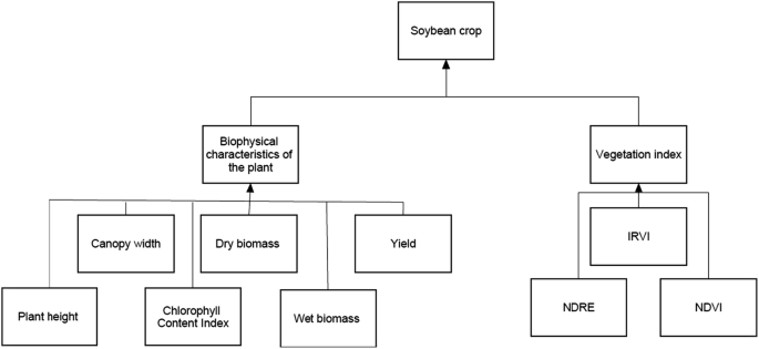
Diagram of the variables analyzed
-
Fresh and dry biomass were collected only from the above-ground of the plant. The samples were obtained using a 0.25 m2 (0.5 × 0.5 m) frame (Fig. 6a). Sampling was conducted per row, for 1 m per point in two rows such that each of these rows was 5 m in length (Fig. 5b). After placing the frames in each of the two rows of the sampling point, the plant was cut at the ground level with the aid of a knife. The aerial part of the soybean was taken, and the roots were discarded. The collected plants were placed in paper bags and weighed to obtain the wet mass (fresh biomass, Fig. 7a), after which the samples were placed in a greenhouse with air circulating at 65 °C for 72 h (Gobbi et al. 2009; Grohs et al. 2009) in order to dry the samples (dry biomass, Fig. 7b). Finally, the dried samples were weighed in a semi-analytical balance (model BL 3200H) to obtain the dry mass.
Fig. 7 
In each collection, wet (a) and dry (b) biomass per sample
-
Chlorophyll index This was obtained using a CCM-200 plus Chlorophyll Content Meter (Marconi, Piracicaba, São Paulo, Brazil) with an accuracy of ± 1 CCI (chlorophyll content index) unit. The readings were performed on three sheets per point and collected randomly; three readings were made per sheet in order to improve data precision.
-
Grain yield The frame used had an area of 0.45 m2, within which plants were cut close to the ground level, before being harvested using a plot combine, which was a Wintersteiger Seedmech Nursey Master Elite® model (Wintersteiger South America, 80240120 Curitiba, PR, Brasil), and then cleaned. Subsequently, the grains were weighed and the data transformed into kg ha−1 (Bertolin et al. 2010).


Statistical analyses
In this study, statistical quality control was managed using control charts, descriptive analysis, and correlation using the Pearson correlation coefficient. Statistical Quality Control, one of the most used tools in the Statistical Process Control (SPC) application, was used to analyze the quality indicators using individual control charts. This tool has been used in several studies, including studies by Chioderoli et al. (2012), Zerbato et al. (2013), and Voltarelli et al. (2015), among others, to enable the monitoring of variation in data over time.
Control charts of individual values were prepared using upper (LSC) and lower (LIC) control limits and the arithmetic mean. These limits were obtained by the mean and standard deviation of the parameter values, with LIC = the mean minus three times the standard deviation, and LSC = the mean plus three times the standard deviation (Toledo et al. 2008). In a normal distribution, 99.7% of the observations are within + or − 3 standard deviations from the mean (Minitab 2017).
Descriptive analyses are simple numerical procedures used to summarize, analyze, organize, and describe the important aspects of a feature set observed in the sample (Pérez-Vicente and Ruiz 2009). Correlation analysis was conducted to verify the behavior of the quality indicators (vegetation indices, fresh and dry biomass, chlorophyll index, canopy width, plant height, and yield). This coefficient is used to measure the intensity, strength, or degree of the linear relationship between two random variables (Stevenson 2001; Bunchaft and Kellner 2002; Barbetta et al. 2004; Kazmier 2007; Ferreira 2009).
The coefficient sign indicates the direction of the correlation and can determine the presence of a linear correlation (Cruz and Regazzi 1997; Cruz and Carneiro 2003; Hair et al. 2005). The values of the correlation coefficient can vary from − 1 to 1, and the higher the value is, the stronger the relationship between the variables is. When the value is close to 0, there is no linear relationship between the variables. However, a value of 1 indicates a perfect linear relationship (Minitab® Support, 2019).
Correlation is one of the statistical analyzes widely applied in the remote sensing area, since it presents the standardized data, is dimensionless and it is also possible to verify the linear relationship between two continuous variables (Minitab 18, 2019), which in this work were the characteristics biophysical studies with vegetation indices. Dancey and Reidy (2006); and Barbetta (2006) describe the classification for the Pearson correlation coefficient: r = 0.10 to 0.30 (weak); r =0.40 to 0.6 (moderate); r = 0.70 to 1 (strong). Thus in this work it was verified which of the biophysical characteristics of the crop that most relate to the vegetation indices.
Spatial and temporal variability maps
The spatial and temporal variability maps were made using the QGIS software, where it was possible to create the maps through the real database collected in the field. The deterministic interpolator Inverse of the Squared Distance (IDW) was used to create the geofields for each biophysical and remote sensing variables collected in the samples area of the crop in the field, allowing visualization and monitoring during soybean crop growth stages (Molin et al. 2015).
where: Z—estimated value for a given point; n—number of neighboring sampling points used in the estimation; Zi—value observed at the sampling point; di—distance between the sampling point and the estimated point (Zi and Z).
Results and discussion
The results and discussion of this study are discussed in the same section. To facilitate the understanding of this section the themes under study are divided into four topics: (i) control charts of individual values, verifying the variability of the process and detecting the processes of reading the vegetation indexes with higher quality; (ii) the descriptive analysis complementing the control charts by dispersion and position values; (iii) correlation between the biophysical variables of the crop and the vegetation indices, observing the optimal time for its use in the field and identifying the indices most correlated with the morphological variables of the soybean; and (iv) maps of spatial and temporal variability for monitoring the growth stages of the soybean crop.
Control of individual values
Using the control charts (Fig. 8) and descriptive analyses, it was possible to monitor the temporal variability of the indices (NDVI, IRVI, and NDRE) as well as the performance of these indices through the canopy sensors. NDRE demonstrated a higher process quality due to its lower variability as compared to NDVI and IRVI, and the lowest values for the coefficients of variation and dispersion.

Control charts showing individual values for the vegetation indices (NDVI, NDRE and IRVI) at 30, 45, 60, 75, and 90 DAS. UCL upper control limit, LCL lower control limit, \(\overline{X}\), average, DAS days after sowing, NDVI normalized difference vegetation index, NDRE normalized difference red-edge index, IRVI inverse ratio vegetation index
In their evaluation of several stages of soybean crop development in 2015 and 2016, Miller et al. (2018) used a canopy sensor with NDRE in order to verify the usefulness of this index for the crop, rather than using NDVI, given the limitations of the latter. The authors concluded that NDRE can be used in conditions in which the vegetative canopy has a higher biomass, and that active canopy sensors can overcome the limitations of passive sensors, such as sensor reading time and interference from cloud presence. This was also observed in the control charts that were produced in this study, in which NDRE presented a higher resistance to saturation readings than did NDVI. In addition, the control charts demonstrated their use as an excellent tool for visualizing the period in which NDVI saturation occurred.
As shown in Fig. 8a, there was a saturation in the NDVI values at 75 and 90 DAS (R4 and R6 stages) as the increase in biomass (Fig. 9b) interfered with the accuracy of the readings (Fig. 7a). The control charts of NVDI showed that there is almost no variability in the process (Fig. 9a), though there was some variability for the wet biomass (Fig. 9b). This indicates the importance of the tool in identification of the saturation point of this index. In two separate studies, Cao et al. (2015, 2016) stated that one of the challenges when using the GreenSeeker sensor is that saturation becomes problematic for NDVI during high and medium biomass conditions. Hence, NDVI is not considered suitable for areas of high yield.

Control charts showing individual values for the NDVI wet biomass at 30, 45, 60, 75, and 90 DAS. UCL upper control limit, LCL lower control limit, \(\overline{X}\), average, DAS days after sowing, NDVI normalized difference vegetation index, NDRE normalized difference red-edge index, IRVI inverse ratio vegetation index
The problem with NDVI saturation was observed by Mutanga and Skidmore (2004), who estimated pasture biomass based on vegetation indices, such as NDVI, calculated using the NIR and red bands. However, they found that these indices had limitations in high density vegetation because of saturation. The same authors indicated that, when the canopy is of high density, pasture biomass can be estimated using wavelengths located in the red-edge region, as these are more accurate than standard NDVI.
The United States Geological Survey (USGS, 2015) proposed that the reason for the saturation problem associated with NDVI saturation is that NDVI is based on a scale of values ranging from − 1 to 1, with the highest values being between 0.6 and 0.9 for dense vegetation. However, Huete et al. (2002) reported that this index begins to lose sensitivity with increase in vegetation density.
The points outside the control limits can be explained by leaf characteristics that interfere with their reflectance, such as the spaces occupied by air and water, pigmentation, and cellular structures, all of which affect the wavelength of incident radiation (Gates et al. 1965). Gausman and Allen (1973) reported on the influence of other factors, such as leaf age, light conditions, maturation, water content, senescence, nodal position, and pubescence.
Bernardes (1987) classified the factors related to the absorption of solar radiation and interception as physiological (functional character, i.e., plant age, nutrients, and leaf water content) and morphological (related to the spatial organization of the leaves, that is, leaf insertion angle, vertical and horizontal leaf distribution, and plant cover density).
Descriptive analysis
Descriptive analyses were performed to verify the spatiotemporal variability of the variables. Table 2 shows the dispersion of the values, which varied significantly over time because the ability of leaves to perform photosynthesis increased from seedling emergence until physiological maturity, while the photosynthetic rate significantly reduced until complete maturation of the plant (Moreira 2012). The same author reported that photosynthesis is related to the amount of radiation absorbed in the visible spectrum (red and blue bands), and senescent leaves reflect more strongly in the visible spectrum than young leaves.
In addition, while increased photosynthesis causes plants to absorb more in the red region as the canopy develops, the reflected radiation also increases in the NIR region (Jensen 2011). This infrared energy is not utilized by photosynthesis, but is used by the plant for molecular vibration or heating (Moreira 2012). In the present study, it possible to observe this behavior of the energy derived from the visible and NIR bands due to the use of these bands in calculating the three indices (Table 1).
The spectral behavior of the vegetation can be influenced by the substrate type and canopy architecture (Novo 2008). This was observed by Luiz and Epiphanio (2001) in spectral behavior of soybean, which was affected by soil reflectance as full soil cover was not achieved, therefore causing a reduction in reflectance. Therefore, at 30 DAS in the initial stages of this study, the coefficient of variation and dispersion values were higher as compared to those of other periods due to the influence of the soil and canopy width.
There has been a considerable increase in the number of studies on the impact of various factors on vegetation spectral behavior, such as canopy variables, data acquisition geometry, canopy height and shape, and practices relating to agriculture and species (Kimes 1983; Guyot, 1984; Valeriano 1992; Gleriani 1994; Ferri 2002; Galvão et al., 2004a, b, 2005, 2006).
Pearson correlation coefficient
Pearson coefficient correlation analysis (Table 3) showed that the strongest correlations occurred at 45 and 60 DAS (V5 and V6 stages) due to the higher physiological development potential of the crop. Hence, the indices were better correlated with the agronomic parameters (fresh and dry biomass, canopy width, chlorophyll index, plant height, and yield).
do Amaral and Molin (2014) also concluded that the most satisfactory canopy sensor results can be acquired and measured when sufficient biomass has accumulated, such as at the end of crop development. The sensors usually show lower sensitivity in their evaluation due the excessive accumulation of biomass as compared to earlier developmental stages. This was also observed in the present study, at 75 and 90 DAS (stages R4 and R6).
The lowest values were observed at 30 DAS (stage V3), and could be due to the influence of the higher soil exposure and smaller canopy width, as compared to the later stages. Moreira (2012) stated that a canopy is considered incomplete when the crop is at the beginning of its vegetative development, because the percentage of vegetation cover on the soil is low and reflected radiation is therefore partly derived from the soil and partly from the vegetation. Hence, low correlation values were obtained in this study because of the influence of the soil on sensor readings.
The parameters that showed the best correlations were fresh and dry biomass, canopy width, the chlorophyll index, and plant height, mainly with respect to NDRE. Similar results were obtained by Portz et al. (2012), who used a canopy sensor at wavelengths in the red-edge and NIR regions and found an improvement in the sensor performance in predicting nitrogen and biomass absorption. do Amaral and Molin (2014) observed that the amount of sugarcane biomass had a higher influence on sensor readings as compared to leaf pigment.
Canopy sensors are an efficient tool for predicting yield (Raun et al. 2001; Teal et al. 2006; Lofton et al. 2012). However, in the present study the correlation values for yield were low. This can be explained by the findings of Raun et al. (2005), Kitchen et al. (2010), and do Amaral and Molin (2014) , who reported on the various uncontrollable factors that can affect yield, thereby influencing the relationship between yield and canopy sensors (such as pest attack, climatic stress, and crop management).
NDRE presented the best correlation values in comparison with NDVI and IRVI. Cao et al. (2015, 2016) and Amaral et al. (2015) observed that vegetation indices using wavelengths in the red-edge region are able to overcome the saturation problem experienced when using NDVI. Ma et al. (2001) found that growth conditions may affect the association of NDVI with soybean yield. For example, optimal conditions may result in improved germination and rapid soil cover for capturing solar radiation, but dry and cold planting can delay emergence and lead to a decreased yield.
Typically, most soils covered by plants exhibit peak absorption at wavelengths in the red region. Hence, NDVI loses its sensitivity to biomass change, which may reflect on yield results (Povh et al. 2008). Li et al. (2010a) and Cao et al. (2015), while evaluating the performance of canopy sensors for wheat crop, observed that the amount of biomass caused saturation problems when using NDVI.
The effect of saturation is related to the built-in normalization effect of calculating the vegetation index, and the type of band chosen (Van Niel and McVicar 2004; Gnyp et al. 2014). Saturation problems can be reduced by using wavelengths with a similar penetration in the plant canopy (Van Niel and McVicar 2004) or similar vegetation index rates (Gnyp et al. 2014).
IRVI has been used to predict biomass in areas with a high vegetative intensity as this index is less susceptible to saturation (Hatfield and Prueger 2010; Li et al. 2010b; Bolfe et al. 2012). NDVI uses the NIR region to estimate crop yield by analyzing biomass composition, and methods based on NDVI that obtain data using reflectance have been widely used in recent years. However, the red-edge band may provide a better fit for models that predict soybean yield (Mourtzinis et al. 2014).
Recent studies have demonstrated the superiority of NDRE models, which yield a 28% increase in the coefficient of determination (R2) when compared with models that use wavelengths in the red region (Eitel et al. 2010). The red-edge band penetrates deeply into the plant canopy and is sensitive to chlorophyll in the upper biomass of the canopy, overcoming the saturation problem inherent in NDVI, and is therefore the preferred vegetation index (Li et al. 2014). Eitel et al. (2010) observed that using the red-edge region increased the ability to estimate variations in chlorophyll content (r2 > 0.73) from when the red-edge was not used (r2 = 0.57).
In addition, it was observed in this study that NDVI and IRVI were inversely proportional to each other (Table 3). This has been explained in a study by Kapp Júnior et al. (2016), who showed that the chlorophyll concentration in leaf tissue influences wavelength reflection in the visible spectrum, and that the lower the application of nitrogen to the plant, the lower the chlorophyll level and solar radiation absorption in the visible range, leading to an increased IRVI and decreased NDVI. Motomiya et al. (2009) also reported that lower amounts of nitrogen input cause a decrease in the leaf expansion rate and chlorophyll and reduces crop development. Therefore, the optimal time to take canopy sensor readings, mainly based on NDRE, was at 45 and 60 DAS (V5 and V6 stages), because of the superior correlations between quality indicators (vegetation indices vs. fresh and dry biomass, canopy width, chlorophyll index, yield, and maturation) during the soybean development stages (Table 3).
Spatial and temporal variability maps
In addition to the above topic, this section contains the spatial–temporal variability maps of the variables. Figures 10 and 11 show that an increase in biomass is associated with the development of the crop, and the values corresponding to 90 DAS (Figs. 10e and 11e) were the highest values of wet and dry biomass. However, a low amount of biomass was observed at some places of the map, which can be explained by the presence of terraces, where there was the accumulation of water after precipitation, as a physical barrier made runoff difficult, affecting soybean growth.

Spatiotemporal distribution of fresh or wet biomass variable (kg ha−1) using IDW (Inverse of squared distance)

Spatiotemporal distribution of the dry biomass variable (kg ha−1) using IDW (Inverse of the squared distance)
The spatial and temporal variability of soybean during crop growth has been shown in Figs. 12, 13, and 14. Few areas had small canopy-width plants and lower plant heights, which can be seen at 30 DAS, as the plant was in the initial stages and had a lower leaf area index (Fig. 14a). As the sowing operation was carried out without the use of autopilot, issues such as machinery trampling plants during the field operations of the soybean, presence of short lines, absence of plants in certain locations due to the difficulty of carrying out the sowing operation without the use of autopilot, absence of systematization of the area, presence of faults and double-spacing, and water accumulation were observed in field when there were the terraces.

Spatiotemporal distribution of the variable canopy width (cm) using IDW (Inverse of the squared distance)

Spatiotemporal distribution of the plant height variable (cm) using IDW (Inverse of the squared distance)

Spatiotemporal distribution of the chlorophyll index variable (CCI) using IDW (Inverse of the squared distance)
The variability of NDVI, NDRE, and IRVI vegetation indices for soybean crop is shown in Figs. 14, 15 and 16. In the early stages of the plant, the index readings were affected, showing high spatial variability (Fig. 15). Moreira (2012) explain that this occur because the crop has a low percentage of vegetation cover of the soil, and a noise is captured by the sensor because part of the reflectance is from the plant and the other from soil. Similar trends were also found by Povh et al. (2008), where the initial stages of the culture were influenced by the soil as a consequence of the failure in the emergence of the plants, due to the low leaf area index. However, the same authors reported that it is possible to accurately determine variation in biomass with the greater development of the above ground biomass due to the better closure of the canopy. (Fig. 17)

Spatiotemporal distribution of the NDVI variable using IDW (Inverse of the squared distance)

Spatiotemporal distribution of the variable NDRE using IDW (Inverse of the squared distance)

Spatiotemporal distribution of the variable IRVI using IDW (Inverse of the squared distance)
In the spatiotemporal distribution maps, the index that showed the better performance was the NDRE, while the NDVI had a saturation problem, and the IRVI did not show good performances, as some map locations showed differences between the readings of NDRE and NDVI indices with IRVI. As for the saturation problem of NDVI, Zanzarini et al. (2013) observed that the NDVI had this limitation factor due to the increase in biomass with fast saturation, according to the growth stage of the crop, reducing the accuracy of the reading due the saturation problem this vegetation index.
Liu (2006) found, using satellite images, that the maximum value of saturation was 0.84. Figure 15c shows that some areas had values between 0.785 and 0.833. In Fig. 15d, there is no variance between the values, since it was seen that NDVI reached saturation at 75 and 90. Hence, NDVI is more suitable in the early stages of. However, the NDRE did not present this problem because this index is not susceptible to saturation. Taskos et al. (2015), when comparing reading efficiency between NDRE and NDVI for grape culture, found that NDRE was less susceptible to saturation than NDVI because of the wavelength in the red-edge region.
Conclusions
By using the control charts, it was found that the lower variability of NDRE resulted in a higher process quality as compared to those for NDVI and IRVI, and it also presented the lowest values for the coefficients of variation. The control charts are valuable tools to identify the moment when saturation occurs for the saturation indexes that are more susceptible to saturation, as was the case with NDVI. Control charts have shown great potential in the visual detection of saturation, which is a problem encountered by the researchers, especially when using red wavelengths such as NDVI. Through the charts it is possible to observe the temporal behavior of the indices knowing at what moment it can be used accurately and when there is its saturation. Given this, new statistical tools are being applied to improve the temporal analysis of remote sensing, since normally the data from the reflectance of objects has nonlinear behavior.
Maps of temporal and spatial variability, NDRE showed better performance, NDVI had a saturation problem, and IRVI did not show good performance possibly because it was obtained by the red and near infrared bands, demonstrating that in the wavelength in red it presented limitation in the final stages of cultivation, and in the red-egde band it was less susceptible to saturation than in the red area.
To capture the spatial variability of soybean crop using canopy sensors, readings should be taken after the plants have completely covered the soil. Overall, the results showed that the optimal time was at 45 and 60 DAS (V5 and V6 plant development stages), based mainly on NDRE, due to the better correlations between quality indicators compared to other stages of soybean development.
In future work, statistical process control may possibly be applied to monitor the quality and variability of other vegetation indices and biophysical characteristics. Meanwhile, it was observed in this article in both control charts and maps, they showed similar results, further emphasizing the adoption of remote sensing charts as a promising statistical tool as has already been found in other areas of agrarian sciences.
References
Abdel-Rahman, E. M., & Ahmed, F. B. (2008). The application of remote sensing techniques to sugarcane (Saccharum spp. hybrid) production: A review of the literature. International Journal of Remote Sensing, 29(13), 3753–3767. https://doi.org/10.1080/01431160701874603.
Ag Leader Technology. (2011). Precision point blog. Retrieved September 13, 2017, from http://www.agleader.com/blog/optrx-crop-sensors-a-tech-support-perspective/.
Alvares, C. A., Stape, J. L., Sentelhas, P. C., de Gonçalves, J. L. M., & Sparovek, G. (2013). Köppen’s climate classification map for Brazil. Meteorologische Zeitschrift, 22(6), 711–728. https://doi.org/10.1127/0941-2948/2013/0507.
Amaral, L. R., Molin, J. P., Portz, G., Finazzi, F. B., & Cortinove, L. (2015). Comparison of crop canopy reflectance sensors used to identify sugarcane biomass and nitrogen status. Precision Agriculture, 16(1), 15–28. https://doi.org/10.1007/s11119-014-9377-2.
Amaral, L. R., Trevisan, R. G., & Molin, J. P. (2018). Canopy sensor placement for variable-rate nitrogen application in sugarcane fields. Precision Agriculture, 19(1), 147–160. https://doi.org/10.1007/s11119-017-9505-x.
Barbetta, P. (2006). Estatística aplicada as ciências sociais. Florianópolis: Editora UFSC.
Barbetta, P. A., Reis, M. M., & Bornia, A. C. (2004). Estatística para cursos de engenharia e informática (2nd ed., p. 410). São Paulo, SP: Atlas.
Bernardes, M. S. (1987). Fotossíntese no dossel das plantas cultivadas. In P. R. Castro (Ed.), Ecologia da produção agrícola (p. 249). Piracicaba, SP: Associação Brasileira para Pesquisa da Potassa e do Fosfato.
Bertolin, D. C., de Sá, M. E., Arf, O., Furlani Junior, E., de Colombo, A. S., & de Carvalho, F. L. B. M. (2010). Aumento da produtividade de soja com a aplicação de bioestimulantes. Bragantia, 69(2), 339–347.
Bolfe, E. L., Batistella, M., & Ferreira, M. C. (2012). Correlação de variáveis espectrais e estoque de carbono da biomassa aérea de sistemas agroflorestais. Pesquisa Agropecuária Brasileira, 47(9), 1261–1269.
Bunchaft, G., & de Kellner, S. R. O. (2002). Estatística sem mistérios (4th ed., Vol. 2, p. 303). Petrópolis, RJ: Vozes.
Buschmann, C., & Nagel, E. (1993). In vivo spectroscopy and internal optics of leaves as basis for remote sensing of vegetation. International Journal of Remote Sensing, 14, 711–722. https://doi.org/10.1080/01431169308904370.
Cao, Q., Miao, Y., Feng, G., Gao, X., Li, F., Liu, B., et al. (2015). Active canopy sensing of winter wheat nitrogen status: An evaluation of two sensor systems. Computers and Electronics in Agriculture, 112, 54–67. https://doi.org/10.1016/j.compag.2014.08.012.
Cao, Q., Miao, Y., Feng, G., Gao, X., Liu, B., Liu, Y., et al. (2017). Improving nitrogen use efficiency with minimal environmental risks using an active canopy sensor in a wheat-maize cropping system. Field Crops Research, 214, 365–372. https://doi.org/10.1016/j.fcr.2017.09.033.
Cao, Q., Miao, Y., Shen, J., Yu, W., Yuan, F., Cheng, S., et al. (2016). Improving in-season estimation of rice yield potential and responsiveness to topdressing nitrogen application with Crop Circle active crop canopy sensor. Precision Agriculture, 17(2), 136–154. https://doi.org/10.1007/s11119-015-9412-y.
Carneiro, F. M. (2018). Sensores de dossel no monitoramento da variabilidade temporal das culturas da soja e do amendoim. 122 f. Tese (Doutorado) - Curso de Agronomia (Produção Vegetal), Universidade Estadual Paulista (Unesp), Faculdade de Ciências Agrárias e Veterinárias, Jaboticabal, Jaboticabal. Disponível em: https://repositorio.unesp.br/handle/11449/155945. Accessed 6 Dec 2019.
Carneiro, F. M., Zerbato, C., Menezes, P. C., Girio, L. A. S., Oliveira, M. F., & Furlani, C. E. A. (2017). Sensoriamento Terrestre. Revista Cultivar Máquinas, 15, 20–21.
Chioderoli, C. A., da Silva, R. P., de Noronha, R. H. F., Cassia, M. T., & dos Santos, E. P. (2012). Perdas de grãos e distribuição de palha na colheita mecanizada de soja. Bragantia, 71(1), 112–121. https://doi.org/10.1590/s0006-87052012005000003.
Ciampitti, I.; Shoup, D.; & Duncan, S. (2014). Late planting of soybeans: Management considerations. Retrieved May 31, 2018, from https://webapp.agron.ksu.edu/agr_social/eu_article.throck?article_id=1429.
Cruz, C. D., & Carneiro, P. C. S. (2003). Modelos biométricos aplicados ao melhoramento genético (p. 585). Viçosa, MG: UFV.
Cruz, C. D., & Regazzi, A. J. (1997). Modelos biométricos aplicados ao melhoramento genético (2nd ed., p. 390). Viçosa, MG: UFV.
Dancey, C., & Reidy, J. (2006). Estatística Sem Matemática para Psicologia: Usando SPSS para Windows (3rd ed., p. 608). Artmed: Porto Alegre.
Novo, E. M. L. M. (2008). Sensoriamento Remoto: Princípios e aplicações (p. 363). São Paulo: Ed. Blucher.
do Amaral, L. R., & Molin, J. P. (2014). The effectiveness of three vegetation indices obtained from a canopy sensor in identifying sugarcane response to nitrogen. Agronomy Journal, 106(1), 273–280.
dos Santos, A. F., da Silva, R. P., Zerbato, C., de Menezes, P. C., Kazama, E. H., Paixão, C. S., et al. (2018). Use of real-time extend GNSS for planting and inverting peanuts. Precision Agriculture. https://doi.org/10.1007/s11119-018-9616-z.
Eitel, J. U., Keefe, R. F., Long, D. S., Davis, A. S., & Vierling, L. A. (2010). Active ground optical remote sensing for improved monitoring of seedling stress in nurseries. Sensors (Basel Switzerland), 10(4), 2843–2850. https://doi.org/10.3390/s100402843.
Embrapa—Empresa Brasileira de Pesquisa Agropecuária. (2013). Sistema Brasileiro de Classificação de Solos (3rd ed. Rev. ampl., p. 353). Brasília, DF: Empresa Brasileira de Pesquisa Agropecuária (Embrapa).
Embratop. Receptor GPS Trimble R6 (L1/L2). 2017. Retrieved November 30, 2018, from http://www.embratop.com.br/produto/receptor-gps-trimble-r6-l1-l2/.
Ferreira, D. F., & Carneiro, D. F. (2009). Estatística básica (2nd ed., p. 664). Lavras, MG: UFLA.
Ferri, C. P. (2002). Utilização da reflectância espectral para a estimativa de pigmentos fotossintéticos em dosséis de soja [Gycine max (L.), Merril]. p. 173. (INPE-8983-TDI/814). Tese (Doutorado em Sensoriamento Remoto)—Instituto Nacional de Pesquisas Espaciais, São José dos Campos.
Fitzgerald, G. J., Rodriguez, D., Christensen, L. K., Belford, R., Sadras, V. O., & Clarke, T. R. (2006). Spectral and thermal sensing for nitrogen and water status in rainfed and irrigated wheat environments. Precision Agriculture, 7, 233–248. https://doi.org/10.1007/s11119-006-9011-z.
Galvão, L. S., Almeida-Filho, R., & Vitorello, I. (2004a). Spectral discimination of hydrothermally altered-materials using ASTER short-wave infrared bands: Evaluation in a tropical savannah environment. International Journal of Applied Earth Observation and Geoinformation, 7(2), 107–114. https://doi.org/10.1016/j.jag.2004.12.003.
Galvão, L. S., Formaggio, A. R., & Tisot, D. A. (2005). Discriminação de variedades de cana-de-açúcar com dados hiperespectrais do sensor Hyperion/EO-1. Revista Brasileira de Cartografia, 57(1), 7–14.
Galvão, L. S., Formaggio, A., & Tisot, D. A. (2006). The influence of spectral resolution on discriminating Brazilian sugarcane varieties. International Journal of Remote Sensing, 27(4), 769–777. https://doi.org/10.1080/01431160500166011.
Galvão, L. S., Ponzoni, F. J., Epiphanio, J. C. N., Formaggio, A. R., & Rudorff, B. F. T. (2004b). Sun and view angle effects on NDVI determination of land cover types in the Brazilian Amazon region with hyperspectral data. International Journal of Remote Sensing, 25(10), 1861–1879. https://doi.org/10.1080/01431160310001598908.
Gates, D. M., Keegan, H. J., Chleter, J. C., & Weidner, V. R. (1965). Spectral properties of plants. Applied Optics, 4(1), 11–20. https://doi.org/10.1364/AO.4.000011.
Gausman, H. W., & Allen, W. A. (1973). Optical parameters of leaves of 30 plant species. Plant Physiology, 52(1), 57–62.
Gitelson, A. A., Merzlyak, M. N., & Lichtenthaler, H. K. (1996). Detection of red edge position and chlorophyll content by reflectance measurements near 700 nm. J. Plant Physiology., 148, 501–508. https://doi.org/10.1016/S0176-1617(96)80285-9.
Gitelson, A. A., Viña, A., Verma, S. B., Rundquist, D. C., Arkebauer, T. J., Keydan, G., et al. (2006). Relationship between gross primary production and chlorophyll content in crops: Implications for the synoptic monitoring of vegetation productivity. Journal of Geophysical Research. https://doi.org/10.1029/2005JD006017.
Gleriani, J. M. (1994). Influência do solo e de fundo e da geometria da radiação na resposta espectral da cultura do feijão. p. 87. (INPE-5632-TDI/556). Dissertação (Mestrado em Sensoriamento Remoto)—Instituto Nacional de Pesquisas Espaciais, São José dos Campos.
Gnyp, M. L., Miao, Y., Yuan, F., Ustin, S. L., Yu, K., Yao, Y., et al. (2014). Hyperspectral canopy sensing of paddy rice aboveground biomass at different growth stages. Field Crops Research, 155, 42–55. https://doi.org/10.1016/j.fcr.2013.09.023.
Gobbi, K. F., Garcia, R., Garcez Neto, A. F., Pereira, O. G., Ventrella, M. C., & Rocha, G. C. (2009). Características morfológicas, estruturais e produtividade do capim-braquiária e do amendoim forrageiro submetidos ao sombreamento. Revista Brasileira de Zootecnia, 38(9), 1645–1654. https://doi.org/10.1590/S1516-35982009000900002.
Grohs, D. S., Bredemeier, C., Mundstock, C. M., & Poletto, N. (2009). Modelo para estimativa do potencial produtivo em trigo e cevada por meio do sensor GreenSeeker. Engenharia Agrícola, 29(1), 101–112. https://doi.org/10.1590/S0100-69162009000100011.
Grohs, D. S., Bredemeier, C., Poletto, N., & Mundstock, C. M. (2011). Validação de modelo para predição do potencial produtivo de trigo com sensor óptico ativo. Pesquisa Agropecuária Brasileira, 46(4), 446–449. https://doi.org/10.1590/S0100-204X2011000400015.
Guo, C., Zhang, L., Zhou, X., Zhu, Y., Cao, W., Qiu, X., et al. (2018). Integrating remote sensing information with crop model to monitor wheat growth and yield based on simulation zone partitioning. Precision Agriculture, 19(1), 55–78. https://doi.org/10.1007/s11119-017-9498-5.
Guyot, G., Hanocq, J. F., Lepne, T., Malet, P., & Verbrugghe, M. (1984). Étude des potentialities de SPOT poor suiure la evolution de couverts de céréales. L’Espace Geographique, 3, 257–264.
Hair, J. F., Anderson, R. E., Tatham, R. L., & Black, W. C. (2005). Análise multivariada de dados (5th ed., p. 593). Porto Alegre, RS: Bookman.
Hansen, P., & Schjoerring, J. (2003). Reflectance measurement of canopy biomass and nitrogen status in wheat crops using normalized difference vegetation indices and partial least squares regression. Remote Sensing of Environment, 86(4), 542–553. https://doi.org/10.1016/S0034-4257(03)00131-7.
Hatfield, J. L., & Prueger, J. H. (2010). Value of using different vegetative indices to quantify agricultural crop characteristics at different growth stages under varying management practices. Remote Sensing, 2(2), 562–578. https://doi.org/10.3390/rs2020562.
Huete, A., Didan, K., Miura, T., Rodriguez, E. P., Gao, X., & Ferreira, L. G. (2002). Overview of the radiometric and biophysical performance of the MODIS vegetation indices. Remote Sensing of Environment, 83(1–2), 195–213. https://doi.org/10.1016/S0034-4257(02)00096-2.
Jensen, J. R. (2011). Sensoriamento remoto do ambiente: uma perspectiva em recursos terrestres. 2. ed. São José dos Campos, SP: Parênteses. p. 598. Tradução de: Epiphanio, J. C. N.; Formaggio, A. R., Santos, A. R. dos, Rudorff, B. F. T., Almeida, C. M. de, & Galvão, L. S.
Jones, H. G., & Vaughan, R. A. (2010). Remote sensing of vegetation: Principles, techniques and applications (p. 353). Oxford: Oxford University Press.
Kapp Júnior, C., Guimarães, A. M., & Caires, E. F. (2016). Use of active canopy sensors to discriminate wheat response to nitrogen fertilization under no-tillage. Engenharia Agrícola, 36(5), 886–894. https://doi.org/10.1590/1809-4430-Eng.Agric.v36n5p886-894/2016.
Kazmier, L. J. (2007). Estatística aplicada à administração e economia (p. 392). Porto Alegre, RS: Bookman.
Kimes, D. S. (1983). Dynamics of directional reflectance factor distributions for vegetation canopies. Applied Optics, 22(9), 1364–1372. https://doi.org/10.1364/AO.22.001364.
Kitchen, N. R., Sudduth, K. A., Drummond, S. T., Scharf, P. C., Palm, H. L., Roberts, D. F., et al. (2010). Ground-based canopy reflectance sensing for variable-rate nitrogen corn fertilization. Agronomy Journal, 102(1), 71–84. https://doi.org/10.2134/agronj2009.0114.
Kumar, R., & Silva, L. (1973). Light ray tracing through a leaf cross section. Applied Optics, 12, 2950–2954. https://doi.org/10.1364/AO.12.002950.
Li, F., Miao, Y., Chen, X., Zhang, H., Jia, L., & Bareth, G. (2010a). Estimating winter wheat biomass and nitrogen status using an active crop sensor. Intelligent Automation and Soft Computing, 16(6), 1221–1230.
Li, F., Miao, Y., Feng, G., Yuan, F., Yue, S., Gao, X., et al. (2014). Improving estimation of summer maize nitrogen status with red edge-based spectral vegetation indices. Field Crops Research, 157, 111–123. https://doi.org/10.1016/j.fcr.2013.12.018.
Li, F., Miao, Y., Henning, S. D., Gnyp, M. L., Chen, X., Jia, L., et al. (2010b). Evaluating hyperspectral vegetation indices for estimating nitrogen concentration of winter wheat at different growth stages. Precision Agriculture, 11(4), 335–357. https://doi.org/10.1007/s11119-010-9165-6.
Lichtenthaler, H. K., & Buschmann, C. (2001). Chlorophylls and carotenoids: Measurement and characterization by UV–vis spectroscopy, current protocols in food analytical chemistry (pp. F4.3.1–F4.3.8). New York: Wiley.
Liu, W. T. H. (2006). Aplicações de sensoriamento remoto (2nd ed., p. 908). Campo Grande: UNIDERP.
Lofton, J., Tubana, B. S., Kanke, Y., Teboh, J., Viator, H., & Dalen, M. (2012). Estimating sugarcane yield potential using an in-season determination of normalized difference vegetative index. Sensors (Basel Switzerland), 12(6), 7529–7547. https://doi.org/10.3390/s120607529.
Luiz, A. J. B., & Epiphanio, J. C. N. (2001). Amostragem por pontos em imagens de sensoriamento remoto para estimativa de área plantada por município. In SIMPÓSIO BRASILEIRO DE SENSORIAMENTO, 10., 2001, Foz do Iguaçu. Anais… São José dos Campos: INPE, 2001, p.111-118. CD-ROM, On-line. ISBN 85-17-00016-1. (INPE-8212-PRE/4001).
Ma, B. L., Dwyer, L. M., Costa, C., Cober, E. R., & Morrison, M. J. (2001). Early prediction of soybean yield from canopy reflectance measurements. Agronomy Journal, 93(6), 1227–1234. https://doi.org/10.2134/agronj2001.1227.
Martins, G. D., & de Galo, M. L. B. T. (2015). Caracterização espectral da cana-de-açúcar infectada por nematoides e migdolus fryanus por espectrorradiometria de campo. Boletim de Ciências Geodésicas, 21(4), 783–796. https://doi.org/10.1590/S1982-21702015000400046.
McFadden, B. R., Brorsen, B. W., & Raun, W. R. (2018). Nitrogen fertilizer recommendations based on plant sensing and Bayesian updating. Precision Agriculture, 19(1), 79–92. https://doi.org/10.1007/s11119-017-9499-4.
Menezes, P. C. D., Silva, R. P. D., Carneiro, F. M., Girio, L. A. D. S., Oliveira, M. F. D., & Voltarelli, M. A. (2018). Can combine headers and travel speeds affect the quality of soybean harvesting operations? Revista Brasileira de Engenharia Agrícola e Ambiental, 22(10), 732–738. https://doi.org/10.1590/1807-1929/agriambi.v22n10p732-738.
Miller, J. J., Schepers, J. S., Shapiro, C. A., Arneson, N. J., Eskridge, K. M., Oliveira, M. C., et al. (2018). Characterizing soybean vigor and productivity using multiple crop canopy sensor readings. Field Crops Research, 216, 22–31. https://doi.org/10.1016/j.fcr.2017.11.006.
Minitab 18. Suporte ao Minitab 18: Distribuição normal. 2017. Retrieved October 2, 2017, from https://support.minitab.com/pt-br/minitab/18/help-and-how-to/probability-distributions-and-random-data/supporting-topics/distributions/normal-distribution/.
Minitab 18. Suporte ao Minitab®18: Visão geral de Correlação. 2019. Retrieved October 1, 2019, from https://support.minitab.com/pt-br/minitab/18/help-and-how-to/statistics/basic-statistics/how-to/correlation/before-you-start/overview/.
Molin, J. P., Amaral, L. R., & Colaço, A. F. (2015). Sensoriamento e sensores. In J. P. Molin, L. R. Amaral, & A. F. Colaço (Eds.), Agricultura de precisão (cap. 5, pp. 119–153). São Paulo, SP: Oficina de Textos.
Montgomery, D. C. (2009). Introduction to statistical quality control (6th ed., p. 754). Hoboken: Wiley.
Moreira, M. A. (2012). Fundamentos do sensoriamento remoto e metodologias de aplicação (4th ed., atual. e ampl., p. 422). Viçosa, MG: UFV.
Motomiya, A. V. A., Molin, J. P., & Chiavegato, E. J. (2009). Utilização de sensor óptico ativo para detectar deficiência foliar de nitrogênio em algodoeiro. Revista Brasileira de Engenharia Agrícola e Ambiental, 13(2), 137–145. https://doi.org/10.1590/S1415-43662009000200005.
Motomiya, A. V. A., Valente, I. M. Q., Molin, J. P., Motomiya, W. R., Biscaro, G. A., & Jordan, R. A. (2014). Índice de vegetação no algodoeiro sob diferentes doses de nitrogênio e regulador de crescimento. Semina: Ciências Agrarias, 35(1), 169–178. https://doi.org/10.5433/1679-0359.2014v35n1p169.
Mourtzinis, S., Rowntree, S. C., Suhre, J. J., Weidenbenner, N. H., Wilson, E. W., Davis, V. M., et al. (2014). The use of reflectance data for in-season soybean yield prediction. Agronomy Journal, 106(4), 1159–1168. https://doi.org/10.2134/agronj13.0577.
Mutanga, O., & Skidmore, A. K. (2004). Narrow band vegetation indices overcome the saturation problem in biomass estimation. International Journal of Remote Sensing, 25(19), 3999–4014.
Pérez-Vicente, S., & Ruiz, M. Expósito. (2009). Descriptive statistics. Allergologia et Immunopathologia, 37(6), 314–320. https://doi.org/10.1016/j.aller.2009.10.005.
Portz, G., Molin, J. P., & Jasper, J. (2012). Active crop sensor to detect variability of nitrogen supply and biomass on sugarcane fields. Precision Agriculture, 13(1), 33–44. https://doi.org/10.1007/s11119-011-9243-4.
Povh, F. P., Molin, J. P., Gimenez, L. M., Pauletti, V., Molin, R., & Salvi, J. V. (2008). Comportamento do NDVI obtido por sensor ótico ativo em cereais. Pesquisa Agropecuária Brasileira, 43(8), 1075–1083. https://doi.org/10.1590/S0100-204X2008000800018.
Raun, W. R., Solie, J. B., Johnson, G. V., Stone, M. L., Lukina, E. V., Thomason, W. E., et al. (2001). In-season prediction of potential grain yield in winter wheat using canopy reflectance. Agronomy Journal, 93(1), 131–138. https://doi.org/10.2134/agronj2001.931131x.
Raun, W. R., Solie, J. B., Stone, M. L., Martin, K. L., Freeman, K. W., Mullen, R. W., et al. (2005). Optical sensor-based algorithm for crop nitrogen fertilization. Communications in Soil Science and Plant Analysis, 36(19–20), 2759–2781. https://doi.org/10.1080/00103620500303988.
Richards, J. A. (1993). Remote sensing digital image analysis: An introduction (p. 340). Berlin: Springer-Verlag Berlin Heidelberg.
Rouse, J. W., Haas, R. H., Schell, J. A., & Deering, D. W. (1973). Monitoring vegetation systems in the great plains with ERTS. In Third earth resources technology satellite-1 symposium (Vol. 1, pp. 309–330).
Rudorff, B. F. T., Aguiar, D. A., Silva, W. F., Sugawara, L. M., Goltz, E., Aulicino, T. L. I. N., et al. (2010). Uso de imagens de satélites de sensoriamento remoto para mapear a área cultivada com cana-de-açúcar no estado de São Paulo—safra 2009/10 (p. 46). São José dos Campos, SP: INPE.
Shiratsuchi, L. S., Brandão, Z. N., Vicente, L. E., de Victoria, D. C., Ducati, J. R., de Oliveira, R. P., et al. (2014). Sensoriamento Remoto: conceitos básicos e aplicações na Agricultura de Precisão. In A. C. C. de Bernardi, J. M. de Naime, A. V. de Resende, L. H. Bassoi, & R. Y. Inamasu (Eds.), Agricultura de precisão: resultados de um novo olhar (cap. 4, pp. 58–73). Brasília, DF: Embrapa.
Silva, V. F. A. (2013). Mobilização do solo e desempenho operacional de semeadora-adubadora com dois tipos de hastes sulcadoras em plantio direto de milho. 60 f. Dissertação (Mestrado)—Curso de Agronomia, Produção Vegetal, Universidade Estadual Paulista (Unesp), Faculdade de Ciências Agrárias e Veterinárias, Jaboticabal.
Stevenson, W. J. (2001). Estatística aplicada à administração (p. 495). São Paulo, SP: Harbra.
Suporte ao Minitab® 18 (2019). Interpretar os principais resultados para Correlação. Retrieved April 18, 2019, from https://support.minitab.com/pt-br/minitab/18/help-and-how-to/statistics/basic-statistics/how-to/correlation/interpret-the-results/key-results/#step-1-examine-the-linear-relationship-between-variables-pearson.
Taskos, D. G., Koundouras, S., Stamatiadis, S., Zioziou, E., Nikolaou, N., Karakioulakis, K., et al. (2015). Using active canopy sensors and chlorophyll meters to estimate grapevine nitrogen status and productivity. Precision Agriculture, 16(1), 77–98. https://doi.org/10.1007/s11119-014-9363-8.
Tavares, T. D. O., Borba, M. A. D. P., de Oliveira, B. R., da Silva, R. P., Voltarelli, M. A., & Ormond, A. T. S. (2018). Effect of soil management practices on the sweeping operation during coffee harvest. Agronomy Journal, 110(5), 1689–1696. https://doi.org/10.2134/agronj2017.10.0598.
Teal, R. K., Tubana, B., Girma, K., Freeman, K. W., Arnall, D. B., Walsh, O., et al. (2006). In-season prediction of corn grain yield potential using normalized difference vegetation index. Agronomy Journal, 98, 1488–1494. https://doi.org/10.2134/agronj2006.0103.
Thenkabail, P., Smith, R. B., & De Pauw, E. (2000). Hyperspectral vegetation indices and their relationships with agricultural crop characteristics. Remote Sensing of Environment, 71(2), 158–182. https://doi.org/10.1016/S0034-4257(99)00067-X.
Toledo, A., Tabile, R. A., da Silva, R. P., Furlani, C. E. A., Magalhâes, S. C., & Costa, B. O. (2008). Caracterização das perdas e distribuição de cobertura vegetal em colheita mecanizada de soja. Engenharia Agrícola, 28(4), 710–719. https://doi.org/10.1590/S0100-69162008000400011.
Trimble—Transforming the Way the World Works.2013. Especificações técnicas. Retrieved November 29, 2017, from http://www.geodata.eng.br/manuais/gps/trimble/R6.pdf.
USGS—United States Geological Survey. (2015). NDVI, the Foundation for Remote Sensing Phenology. United States Geological Survey. Retrieved May 31, 2018, from https://phenology.cr.usgs.gov/ndvi_foundation.php.
Valeriano, M. M. (1992). Reflectância espectral do trigo irrigado (Triticum aestivum, L.) por espectrorradiometria de campo e aplicação do modelo SAIL. 1992-05. p. 149 (INPE-5426-TDI/483). Dissertação (Mestrado em Sensoriamento Remoto)—Instituto Nacional de Pesquisas Espaciais, São José dos Campos.
Van Niel, T. G., & McVicar, T. R. (2004). Current and potential uses of optical remote sensing in rice-based irrigation systems: A review. Australian Journal of Agricultural Research, 55(2), 155–185. https://doi.org/10.1071/AR03149.
Voltarelli, M. A., da Silva, R. P., Cassia, M. T., Ortiz, D. F., & Torres, L. S. (2015). Qualidade do corte basal de cana-de-açúcar utilizando-se de três modelos de facas. Engenharia Agrícola, 35(3), 528–541. https://doi.org/10.1590/1809-4430-Eng.Agric.v35n3p528-541/2015.
Zanzarini, F. V., Pissarra, T. C. T., Brandão, F. J. C., Teixeira, D. D. B. (2013). Correlação espacial do índice de vegetação (NDVI) de imagem Landsat/ETM+com atributos do solo. Revista Brasileira de Engenharia Agrícola e Ambiental, 17(6), 608–614. https://doi.org/10.1590/S1415-43662013000600006.
Zerbato, C., Cavichioli, F. A., Raveli, M. B., Marrafon, M., & da Silva, R. P. (2013). Controle Estatístico de Processo aplicado à colheita mecanizada de milho. Engenharia na agricultura, 21(3), 261–270.
Zerbato, C., Furlani, C. E. A., Ormond, A. T. S., da Silva Gírio, L. A., Carneiro, F. M., & da Silva, R. P. (2017). Statistical process control applied to mechanized peanut sowing as a function of soil texture. PLoS ONE, 12(7), e0180399. https://doi.org/10.6084/m9.figshare.4204665.
Author information
Authors and Affiliations
Corresponding author
Ethics declarations
Conflict of interest
The authors declare that they have no conflict of interest.
Additional information
Publisher's Note
Springer Nature remains neutral with regard to jurisdictional claims in published maps and institutional affiliations.
Rights and permissions
About this article

Cite this article
Morlin Carneiro, F., Angeli Furlani, C.E., Zerbato, C. et al. Comparison between vegetation indices for detecting spatial and temporal variabilities in soybean crop using canopy sensors. Precision Agric 21, 979–1007 (2020). https://doi.org/10.1007/s11119-019-09704-3
Published:
Issue Date:
DOI: https://doi.org/10.1007/s11119-019-09704-3