
Abstract
In the present article, an Extended Trial Equation method has been applied to derive the new exact solutions for generalized form of equations. We consider ZK equation and ZK-BBM equation to demonstrate the features and credibility of the suggested technique. As a result, many new exact soliton solutions are obtained, which includes rational solutions, soliton type solutions, and singular soliton solutions. These types of solutions might perform significant role in engineering domains.
1 Introduction
In recent years, Soliton solutions of nonlinear evolution equations plays an important part in the study of nonlinear complex physical phenomena and one of the most empowering and extremely active area of research investigation. Which appears in various fields of physical sciences such as solid state physics, plasma physics, relativity, optical fibers, biomechanics, and ecology. A search of direct approach for exact solutions of nonlinear equations has become more and more attractive in recent years because of the availability of computer symbolic systems like Maple or Mathematica.
Several methods including Auxiliary Equation (Kumar et al. 2008; Liu and Liu 2009), Variational Iteration (Mohyud-Din et al. 2011), Solitary wave ansatz (Zayed and Al-Nowehy 2016), Modified Simple Equation (Jawad et al. 2010; Zayed 2011; Zayed and Hoda Ibrahim 2012, 2013), Trigonometric function series (Zhang 2008), Jacobi elliptic function (Yan 2003), Sine–Cosine (Wazwaz 2004; Borhanifar et al. 2008, 2009, 2010; Filiz Taşcan 2009), first integral (Eslami et al. 2014; Mirzazadeh and Biswas 2014; Darvishi et al. 2016), exp (−φ(ξ))-expansion method (Khater 2016), Tanh (Wazwaz 2008a), Extended Tanh (Khater et al. 2017; Zahran and Khater 2016; Lü and Chen 2015; Shukri and Al-Khaled 2010), F-expansion (Yomba 2004, 2005; Wang and Li 2005a, b; Ren and Zhang 2006; Zhang et al. 2006; Abdou 2007), Exp-function (Wu and He 2006; Bekir and Boz 2008; Zhou et al. 2008; Borhanifar et al. 2009; Borhanifar and Kabir 2009; Guner and Atik 2016), \(\left( {\frac{{G^{\prime } }}{G}} \right)\)-expansion method (Wang et al. 2008; Zhang et al. 2008; Liu 2005), Trail Equation (Du 2010; Bulut 2013), Extended Trial Equation (Gurefe et al. 2013; Pandir 2014; Mirzazadeh et al. 2016) have been used to find appropriate solutions of nonlinear partial differential equations. Inspired and motivated by the ongoing research in this area, We apply Extended Trial Equation method on generalized ZK equation (gZK) (Wazwaz 2008b) and generalized ZK-BBM equation (Wazwaz 2005):
and
where α and β are arbitrary constants. The ZK equation in two-dimension, was first derived for describing weakly nonlinear ion-acoustic waves in a polarized lossless plasma. While generalized ZK-BBM equation developed to the ZK Equation, imitative from standard BBM equation, its normally called generalized form of ZK-BBM equation. Moreover, in earlier literature the Extended Trial Equation method has not been applied to the above suggested equations. Wazwaz (2008b) studied generalized ZK equation by utilizing the Extended Tanh method. Wazwaz (2005) investigated generalized ZK-BBM equation via the Sine–Cosine method and Tanh method etc. The main merits of Extended Trial Equation method over the other techniques are that it gives more general solutions with a few constants and presents a wider applicability for handling nonlinear evolution equations (NLEEs) in a direct manner without any initial/boundary condition at the outset.
It is to be highlighted that, we use Extended Trial Equation method with complete discrimination system for polynomials in which balance number is not constant as we have in other methods. If the balance number is not constant then we get many solutions, but we suppose some of these solutions. By this approach, we obtain the analytical solutions of ZK and ZK-BBM equation with generalized evolution in mathematical physics, not use any specific value for \(\varvec{n}\) to obtain solutions. In this article, we not only discussed basic features of 1-soliton solution and singular soliton solution by analytically but also considered numerically in the form of graphs, and results are compared by substituting different values for \(\varvec{n}\), and obtained different new solutions numerically.
The paper is organized as follows: in Sect. 2, we give the numerical Scheme of the Extended Trial Equation method to obtain abundant exact solitary solutions. To demonstrate the technique, generalized ZK equation and generalized ZK-BBM equation are examined in Sect. 3. Furthermore, we finish up the paper in the last section
2 Extended Trial Equation method
The basic strategy of the technique can understand by the following strides:
-
Step I. We assume that the given nonlinear PDE
$$H\left( {u,u_{t} , u_{x} , u_{y} ,u_{z} , u_{xx} ,u_{yy} u_{xt} , u_{tt} , \ldots } \right) = 0,$$(1)Utilizing the wave transformation
$$u\left( {x_{1} , \ldots ,x_{N} ,t} \right) = u\left( \eta \right),\quad \eta = \lambda \left( {\sum\limits_{j = 1}^{N} {x_{j} - ct} } \right),$$where c ≠ 0 and λ ≠ 0. The wave transformation changes Eq. (1) into a nonlinear ODE.
$$Q\left( {u,u^{\prime } , - \mu u^{\prime } ,u^{\prime \prime } , \mu^{2} u^{\prime \prime } , \ldots } \right) = 0,$$(2) -
Step II. The solution of Eq. (1) has the following generalized form.
$$u\left( \eta \right) = \sum\limits_{i = 0}^{\delta } {\tau_{i}\Gamma ^{i} } ,$$(3)where
$$\left( {\Gamma^{\prime } } \right)^{2} =\Omega (\Gamma ) = \frac{{\upphi(\Gamma )}}{{\uppsi(\Gamma )}} = \frac{{\xi_{\theta } \Gamma^{\theta } + \cdots + \xi_{1} \Gamma + \xi_{0} }}{{\zeta_{\sigma } \Gamma^{\sigma } + \cdots + \zeta_{1} \Gamma + \zeta_{0} }},$$(4)$$\left( {u^{\prime } } \right)^{2} = \frac{{\upphi(\Gamma )}}{{\uppsi(\Gamma )}}\left( {\sum\limits_{i = 0}^{\delta } {i\tau_{i} \Gamma^{i - 1} } } \right)^{2} ,$$(5)$$\left( {u^{\prime \prime } } \right) = \frac{{\upphi^{\prime } (\Gamma )\uppsi(\Gamma ) -\upphi(\Gamma )\uppsi^{\prime } (\Gamma )}}{{2\uppsi^{2} (\Gamma )}}\left( {\sum\limits_{i = 0}^{\delta } {i\tau_{i} \Gamma^{i - 1} } } \right) + \frac{{\upphi(\Gamma )}}{{\uppsi(\Gamma )}}\left( {\sum\limits_{i = 0}^{\delta } {i\left( {i - 1} \right)\tau_{i} \Gamma^{i - 2} } } \right).$$(6)In above equations, given \(\upphi(\Gamma )\) and \(\uppsi(\Gamma )\) are polynomials. Using Eqs. (5) and (6) into Eq. (2) yields a polynomial as:
$$\chi \left( \Gamma \right) = {\varrho }_{s} \Gamma^{s} + \cdots + {\varrho }_{1} \Gamma + {\varrho }_{0} = 0.$$(7)We can determine a formula of \(\theta , \sigma\) and δ by using the balance principle technique and can find some estimations of \(\theta , \sigma\) and δ.
-
Step III. Setting each coefficient of polynomial \(\chi (\Gamma )\) to zero to derive system of algebraic equations:
$${\varrho }_{i} = 0,\quad i = 0, \ldots ,s.$$(8)Now we will determine the values of \(\xi_{0} , \ldots ,\xi_{\theta } ,\quad \zeta_{0} , \ldots ,\zeta_{\sigma }\) and τ 0, …, τ δ , by simplification of the above system of equations.
-
Step IV. In the following step, we obtain elementary form of integral by reduction of Eq. (4), as follows
$$\pm \left( {\eta - \eta_{0} } \right) = \int {\frac{d\Gamma }{{\sqrt {\Omega \left( \Gamma \right)} }}} = \int {\sqrt {\frac{{{\uppsi }(\Gamma )}}{{{\upphi }(\Gamma )}}} } d\Gamma$$(9)where η 0 is an arbitrary constant. We can classify the roots of \({\upphi }(\Gamma ),\) with the help of complete discrimination system for polynomials. We solve Eq. (9), by using Maple or Mathematica and acquire the solutions to Eq. (1).
3 Solution procedure
3.1 Generalized ZK equation
Generalized form of ZK equation (Wazwaz 2008b) read:
Now, we utilize the wave variable u(x, y, t) = u(η), η = x + y − ct, Eq. (10) in three independent variables is changing into the following ODE:
Obtained by integrating the resulting equation and considering each constant of integration to be zero. Now applying the following transformation
The transformation in Eq. (12) will transform Eq. (11) into the ODE
In Eq. (13), when substitute Eqs. (5), (6) and use balance principle technique, we get
If we take into consideration \(\sigma = 0,\theta = 3\) and δ = 1, we can get solutions of Eq. (10), as follows
where \(\zeta_{0} \ne 0\;{\text{and}}\;\xi_{3} \ne 0.\) Individually, solving the algebraic equation system (8) with the aid of Maple 2016, yields
Substituting Eq. (17) into Eqs. (4) and (9), we have
where
By integrating (18), we acquire the solutions to the (10) as:
where
Also \(\alpha_{1} , \alpha_{2} ,\alpha_{3}\) are solutions of the polynomial equation
where \(r_{2} = \frac{{\xi_{2} }}{{\xi_{3} }},r_{1} = \frac{{\xi_{1} }}{{\xi_{3} }}\) and \(r_{0} = \frac{{\xi_{0} }}{{\xi_{3} }}\).
Substituting the solutions given in Eqs. (19)–(21) into (3) and (12), as follows
Denoting \(\bar{\tau } = \tau_{0} + \tau_{1} \alpha_{1} ,\) and setting, respectively
If we take τ 0 = −τ 1 α 1, and η 0 = 0, for simplicity, then the solutions given in Eqs. (24)–(26) can be written in the following types:
-
Rational solution
$$u\left( {x, y, t} \right) = \left[ {\frac{{2\sqrt {\tau_{1} A} }}{x + y - pt}} \right]^{{\frac{2}{n}}} ,$$(27) -
1-Soliton solution
$$u\left( {x,y,t} \right) = \frac{{E_{1} }}{{cosh^{{\frac{2}{n}}} \left[ { \mp G(x + y - pt} \right]}},$$(28) -
Singular soliton solution
$$u\left( {x,y,t} \right) = \frac{{E_{2} }}{{sinh^{{\frac{2}{n}}} \left[ {G(x + y - pt} \right]}},$$(29)where
$$E_{1} = \left[ {\tau_{1} (\alpha_{2} - \alpha_{1} )} \right]^{{\frac{1}{n}}} ,\quad E_{2} = \left[ {\tau_{1} (\alpha_{2} - \alpha_{1} )} \right]^{{\frac{1}{n}}} ,\quad G = \frac{1}{2}\sqrt {\frac{{\alpha_{1} - \alpha_{2} }}{A}} .$$Here G is called the inverse width of the solitons, p the velocity. While amplitudes of the solitons represented by E 1 and E 2. Hence, we can say that the soliton occurs for τ 1 > 0 (Figs. 1, 2).
Fig. 1 
Solution of Eq. (28) corresponding to the values \(n = 2,n = 3,n = 4\) from left to right with \(E_{1} = 4,B = 1,c = 1\)
Fig. 2 
Solution of Eq. (29) corresponding to the values \(n = 2,n = 3,n = 4\) from left to right with \(E_{2} = 4,B = 1,c = 1\)


3.2 Generalized ZK-BBM equation
Generalized form of ZK-BBM equation (Wazwaz 2005) read:
Right now, we will make use of the travelling wave variable in (30)
We get the desired equation by integration the transformed ODE and setting each integration constant to zero.
Equation (31) becomes
In Eq. (33), when substitute Eqs. (5), (6) and use balance principle technique, we get
If we consider \(\sigma = 0, \theta = 3\) and \(\delta = 1,\) then
where \(\zeta_{0} \ne 0,\xi_{3} \ne 0\). Respectively, solving the algebraic equation system (8) using Maple 2016, we get
putting Eq. (37) into Eqs. (4) and (9), we have
where
By integrating (38), we obtain the solutions to the Eq. (30) as follows
where
Also \(\alpha_{1} , \alpha_{2} ,\alpha_{3}\) are solutions of the polynomial equation
where \(r_{2} = \frac{{\xi_{2} }}{{\xi_{3} }}, r_{1} = \frac{{\xi_{1} }}{{\xi_{3} }}\) and \(r_{0} = \frac{{\xi_{0} }}{{\xi_{3} }}\).
Substituting the solutions (39)–(41) into Eq. (3) and Eq. (32).Denoting \(\bar{\tau } = \tau_{0} + \tau_{1} \alpha_{1} ,\) and setting
We find, respectively
If we take τ 0 = −τ 1 α 1, that is \(\bar{\tau } = 0\),then the solutions given in Eqs. (44)–(46) can be written in the following types:
-
Rational solution
$$u\left( {x,y,t} \right) = \left[ {\frac{{2\sqrt {\tau_{1} A} }}{x + y - mt}} \right]^{{\frac{2}{n - 1}}} ,$$(47) -
1-Soliton solution
$$u\left( {x,y,t} \right) = \frac{{E_{1} }}{{cosh^{{\frac{2}{n - 1}}} \left[ { \mp G(x + y - mt} \right]}},$$(48) -
Singular soliton solution
$$u\left( {x,y,t} \right) = \frac{{E_{2} }}{{sinh^{{\frac{2}{n - 1}}} \left[ {G(x + y - mt} \right]}},$$(49)where
$$E_{1} = \left[ {\tau_{1} (\alpha_{2} - \alpha_{1} )} \right]^{{\frac{1}{n - 1}}} ,\quad E_{2} = \left[ {\tau_{1} (\alpha_{2} - \alpha_{1} )} \right]^{{\frac{1}{n - 1}}} ,\quad G = \frac{1}{2}\sqrt {\frac{{\alpha_{1} - \alpha_{2} }}{A}} .$$Here G is called the inverse width of the solitons, m the velocity. While amplitudes of the solitons represented by E 1 and E 2. Hence, we can say that the soliton occurs for τ 1 > 0 (Figs. 3, 4).
Fig. 3 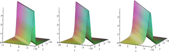
Solution of Eq. (48) corresponding to the values \(n = 2,n = 3\) and n = 4 from left to right with \(E_{1} = 4,B = 1,c = 1\)
Fig. 4 
Solution of Eq. (49) corresponding to the values \(n = 2,n = 3\) and \(n = 4\) from left to right with \(E_{2} = 4,B = 1,c = 1\)


4 Conclusions
In this work, we obtained more general wave solutions of generalized ZK equation and generalized ZK-BBM equation by using the Extended Trial Equation method. Through this technique some renowned equations were tackled. The overall performance of the Extended Trial Equation methods reliable and effective. Furthermore, our obtained results are in more general form. With the support of Maple 2016, we have guaranteed the correctness of the obtained results by substituting them back into the nonlinear partial differential equations. The solutions acquired in this article might have significant impact on future researchers.
References
Abdou, M.A.: The extended F-expansion method and its application for a class of nonlinear evolution equations. Chaos, Solitons Fractals 31, 95–104 (2007)
Bekir, A., Boz, A.: Exact solutions for nonlinear evolution equations using Exp-function method. Phys. Lett. A 372(10), 1619–1625 (2008)
Borhanifar, A., Kabir, M.M.: New periodic and soliton solutions by application of Exp-function method for nonlinear evolution equations. Comput. Appl. Math. 229, 158–167 (2009)
Borhanifar, A., Jafari, H., Karimi, S.A.: New solitons and periodic solutions for the Kadomtsev–Petviashvili equation. Nonlinear Sci. Appl. 4, 224–229 (2008)
Borhanifar, A., Jafari, H., Karimi, S.A.: New solitary wave solutions for the bad Boussinesq and good Boussinesq equations. Numer. Methods Partial Differ. Equ. 25, 1231–1237 (2009a)
Borhanifar, A., Kabir, M.M., Maryam Vahdat, L.: New periodic and soliton wave solutions for the generalized Zakharov system and (2 + 1)-dimensional Nizhnik–Novikov–Veselov system. Chaos, Solitons Fractals 42, 1646–1654 (2009b)
Borhanifar, A., Jafari, H., Karimi, S.A.: New solitary wave solutions for generalized regularized long-wave equation. Int. J. Comput. Math. 87, 509–514 (2010)
Bulut, H.: Classification of exact solutions for generalized form of K(m, n) equation. Abstr. Appl. Anal. 2013, 11 (2013)
Darvishi, M.T., Arbabi, S., Najafi, M., Wazwaz, A.M.: Traveling wave solutions of a (2 + 1)-dimensional Zakharov-like equation by the first integral method and the tanh method. Optik Int. J. Light Electron Opt. 127(16), 6312–6321 (2016)
Du, X.H.: An irrational trial equation method and its applications. Pramana J. Phys. 75(3), 415–422 (2010)
Eslami, M., Mirzazadeh, M., Vajargah, B.F., Biswas, A.: Optical solitons for the resonant nonlinear Schrödinger’s equation with time-dependent coefficients by the first integral method. Optik Int. J. Light Electron Opt. 125(13), 3107–3116 (2014)
Filiz Taşcan, Ahmet Bekir: Analytic solutions of the (2 + 1)-dimensional nonlinear evolution equations using the Sine–Cosine method. Appl. Math. Comput. 215(8), 3134–3139 (2009)
Guner, O., Atik, H.: Soliton solution of fractional-order nonlinear differential equations based on the Exp-function method. Optik Int. J. Light Electron Opt. 127(20), 10076–10083 (2016)
Gurefe, Y., Misirli, E., Sonmezoglu, A., Ekici, M.: Extended Trial Equation method to generalized nonlinear partial differential equations. Appl. Math. Comput. 219(10), 5253–5260 (2013)
Jawad, A.J.M., Petkovic, M.D., Biswas, A.: Modified simple equation method for nonlinear evolution equations. Appl. Math. Comput. 217, 869–877 (2010)
Khater, M.M.A.: Solitary wave solutions for the generalized Zakharov Kuznetsov–Benjamin–Bona–Mahony nonlinear evolution equation. Global J. Sci. Front. Res. Phys. Space Sci. 16(4) (2016) (Ver. 1.0)
Khater, M.M.A., Lu, D., Zahran, E.H.M.: Solitary wave solutions of the Benjamin–Bona–Mahoney–Burgers equation with dual power-law nonlinearity. Appl. Math. Inf. Sci. 11(5), 1–5 (2017)
Kumar, R., Kaushal, R.S., Prasad, A.: Some new solitary and travelling wave solutions of certain nonlinear diffusion-reaction equations using auxiliary equation method. Phys. Lett. A 372, 3395–3399 (2008)
Liu, C.S.: Trial equation method and its applications to nonlinear evolution equations. Acta Phys. Sin. Chin. 54(6), 2505–2509 (2005)
Liu, X.P., Liu, C.P.: Chaos, Solitons Fractals 39, 1915–1919 (2009)
Lü, Z., Chen, Y.: Constructing rogue wave prototypes of nonlinear evolution equations via a extended tanh method. Chaos, Solitons Fractals 81, 218–223 (2015)
Mirzazadeh, M., Biswas, A.: Optical solitons with spatio-temporal dispersion by first integral approach and functional variable method. Optik Int. J. Light Electron Opt. 125(19), 5467–5475 (2014)
Mirzazadeh, M., Ekici, M., Sonmezoglu, A., Zhou, Q., Triki, H., Moshokoa, S.P., Biswas, A., Belic, M.: Optical solitons in birefringent fibers by Extended Trial Equation method. Optik Int. J. Light Electron Opt. 127(23), 11311–11325 (2016)
Mohyud-Din, S.T., Yildirim, A., Demirli, G.: Analytical solution of wave system in with coupling controllers. Int. J. Numer. Method Heat Fluid Flow 21(2), 198–205 (2011)
Pandir, Y.: New exact solutions of the generalized Zakharov–Kuznetsov modified equal-width equation. Pramana J. Phys. 82(6), 949–964 (2014)
Ren, Y.J., Zhang, H.Q.: A generalized F-expansion method to find abundant families of Jacobi elliptic function solutions of the (2 + 1)-dimensional Nizhnik–Novikov–Veselov equation. Chaos, Solitons Fractals 27, 959–979 (2006)
Shukri, S., Al-Khaled, K.: The extended tanh method for solving systems of nonlinear wave equations. Appl. Math. Comput. 217(5), 1997–2006 (2010)
Wang, M.L., Li, X.Z.: Extended F-expansion method and periodic wave solutions for the generalized Zakharov equations. Phys. Lett. A 343, 48–54 (2005a)
Wang, M.L., Li, X.Z.: Applications of F-expansion to periodic wave solutions for a new Hamiltonian amplitude equation. Chaos, Solitons Fractals 24, 1257–1268 (2005b)
Wang, M.L., Zhang, J.L., Li, X.Z.: The G′/G-expansion method and travelling wave solutions of nonlinear evolution equations in mathematical physics. Phys. Lett. A 372, 417–423 (2008)
Wazwaz, A.M.: A Sine–Cosine method for handling nonlinear wave equations. Math. Comput. Model. 40, 499–508 (2004)
Wazwaz, A.M.: Compact and noncompact physical structures for the ZK-BBM equation. Appl. Math. Comput. 169, 713–725 (2005)
Wazwaz, A.M.: The tanh method for travelling wave solutions to the Zhiber–Shabat equation and other related equations. Commun. Nonlinear Sci. Numer. Simul. 13(3), 584–592 (2008a)
Wazwaz, A.M.: The extended tanh method for the Zakharov–Kuznetsov (ZK) equation, the modified ZK equation, and its generalized forms. Commun. Nonlinear Sci. Numer. Simul. 13, 1039–1047 (2008b)
Wu, H.X., He, J.H.: Exp-function method and its application to nonlinear equations. Chaos, Solitons Fractals 30, 700–708 (2006)
Yan, Z.: Abunbant families of Jacobi elliptic function solutions of the (2 + 1)-dimensional integrable Davey–Stewartson-type equation via a new method. Chaos, Solitons Fractals 18, 299–309 (2003)
Yomba, E.: Construction of new soliton-like solutions for the (2 + 1) dimensional Kadomtsev–Petviashvili equation. Chaos, Solitons Fractals 22, 321–325 (2004)
Yomba, E.: Construction of new solutions to the fully nonlinear generalized Camassa–Holm equations by an indirect F-function method. J. Math. Phys. 46, 123504–123512 (2005)
Zahran, M.H.M., Khater, M.M.A.: Modified extended tanh-function method and its applications to the Bogoyavlenskii equation. Appl. Math. Model. 40, 1769–1775 (2016)
Zayed, E.M.E.: A note on the modified simple equation method applied to Sharma Tasso–Olver equation. Appl. Math. Comput. 218, 3962–3964 (2011)
Zayed, E.M.E., Al-Nowehy, A.G.: The solitary wave ansatz method for finding the exact bright and dark soliton solutions of two nonlinear Schrödinger equations. J. Assoc. Arab Univ. Basic Appl. Sci. (2016) (article in press)
Zayed, E.M.E., Hoda Ibrahim, S.A.: Exact solutions of nonlinear evolution equation in mathematical physics using the modified simple equation method. Chin. Phys. Lett. 29, 060201–060204 (2012)
Zayed, E.M.E., Hoda Ibrahim, S.A.: Modified simple equation method and its applications for some nonlinear evolution equations in mathematical physics. Int. J. Comput. Appl. 67, 39–44 (2013)
Zhang, Z.Y.: New exact traveling wave solutions for the nonlinear Klein–Gordon equation. Turk. J. Phys. 32, 235–240 (2008)
Zhang, J.L., Wang, M.L., Wang, Y.M., Fang, Z.D.: The improved F-expansion method and its applications. Phys. Lett. A 350, 103–109 (2006)
Zhang, S., Tong, J.L., Wang, W.: A generalized G′/G-expansion method for the mKdV equation with variable coefficients. Phys. Lett. A 372, 2254–2257 (2008)
Zhou, X.W., Wen, Y.X., He, J.H.: Exp-function method to solve the nonlinear dispersive k(m, n) equations. Int. J. Nonlinear Sci. Numer. Simul. 9, 301–306 (2008)
Acknowledgement
Authors are highly grateful to the unknown referees for their valuable comments.
Author information
Authors and Affiliations
Corresponding author
Rights and permissions
About this article

Cite this article
Mohyud-Din, S.T., Irshad, A. Solitary wave solutions of some nonlinear PDEs arising in electronics. Opt Quant Electron 49, 130 (2017). https://doi.org/10.1007/s11082-017-0974-y
Received:
Accepted:
Published:
DOI: https://doi.org/10.1007/s11082-017-0974-y