
Abstract
At present, a lot of image cryptosystems with permutation/diffusion architecture have been proposed. However, permutation and diffusion are considered as two separate stages, both requiring image-scanning to obtain pixel values. Moreover, because of extraction bits directly from the discrete state value of a chaotic map to generate the pseudorandom binary sequence, the quite time-consuming conversion from floating points to integers cannot be avoided in practical applications. In this paper, a novel image encryption scheme for both combining permutation–diffusion and avoiding conversion of floating-point number is proposed. Firstly, using the lookup table constructed and S-Box of AES, an efficient approach of generating the pseudorandom sequence required by diffusion is proposed. Then, the combined permutation/diffusion architecture is employed to shuffle and change the pixels. Theoretical analyses and computer simulations both confirm that the new algorithm has high security and is very fast for practical image encryption.
1 Introduction
With the rapid growth of image transmission through Internet, the secure transmission of confidential digital images over public channels has become a common interest in both research and application fields. Although some traditional ciphers such as DES and AES are designed with good permutation and diffusion properties, they are generally difficult to handle the image encryption because of some intrinsic properties of images such as bulk data volume and high pixel correlation. Nevertheless, many new image encryption schemes have been proposed in recent years, among which the chaos-based approach appears to be a promising direction [1–15].
In [2], Fridrich suggested that a chaos-based image encryption scheme should compose of the iteration of two processes: permutation and diffusion, namely permutation–diffusion architecture, as shown in Fig. 1.

Architecture of image encryption based on permutation and diffusion
The permutation stage permutes all the pixels as a whole, without changing their values. In the diffusion stage, the pixel values are modified sequentially so that a tiny change in a pixel spreads out to as many pixels in the cipher-image as possible. To eliminate the correlation between adjacent pixels, the whole permutation/diffusion process repeats for a number of times in order to achieve a satisfactory level of security. In Fig. 1, permutation and diffusion are two separate and iterative stages, and they both require scanning the image in order to obtain the pixel value. Thus, at least twice scanning the same image is required in each round of the permutation–diffusion operation. This scanning process is actually repeated but can be avoided if the permutation and diffusion operations be combined, i.e., via changing the values of the pixels while relocating them as illustrated in Fig. 2. As a result, the image only needs to be scanned once so that the encryption speed and efficiency is significantly improved.

Architecture of image encryption combining permutation/diffusion
On the other hand, some chaos-based image encryption algorithms with permutation–diffusion structure are also attacked [13, 16–19, 21, 22].
The common flaws or deficiencies of these algorithms are summarized as follows:
-
(1)
The keystream for encryption/decryption is independent of the plain-image, and this favors known-plaintext and chosen-plaintext attacks.
-
(2)
In the diffusion process, the pseudorandom binary sequence is extracted directly from the discrete state value of a chaotic map. This means that the conversion from floating points to integers cannot be avoided in practical applications. However, it is found from computer simulations that the conversion process is quite time-consuming [5].
In [5], authors proposed a new fast image encryption. Although it can partly avoid to extract bits operation from the discrete state value of a chaotic map, \(N^{2}/8\) times extracting operation cannot yet be avoided in each encryption round. In this paper, we propose a novel scheme for both combining permutation–diffusion and avoiding the conversion of floating-point number. Firstly, using the lookup table constructed and S-Box of AES, an efficient approach of generating the pseudorandom sequence required by diffusion is proposed. Then, the combined permutation/diffusion architecture is employed to shuffle and change the pixels.
The rest of this paper is organized as follows. In Sect. 2, the process of generating pseudorandom binary sequence is described in detail. Section 3 focuses on the description of the proposed fast image encryption. Performance and security of this scheme are analyzed in Sect. 4. In Sect. 5, a conclusion is drawn.
2 The keystream generator
2.1 Generating the pseudorandom sequences
To avoid the float-point operation of extracting in generating the pseudorandom number sequences, an approach of generating the pseudorandom sequence is proposed in this paper as shown in Fig. 3. The 1D chaotic tent map is defined by the following equation:
where \({0<a<1}\). This function maps the interval [0, 1] onto itself with only one parameter \(a\). A sequence formed by iterating \(T_{\alpha }\) from an arbitrary initial point in (0, 1) exhibits chaotic properties [23–26] when \(T_{\alpha }\) is expanding everywhere in the interval (0, 1).

Architecture of generating the pseudorandom sequences
The detail of generating the pseudorandom sequence is described as follow.
- Step 1 :
-
Partition interval [0, 1] into 256 the same length subintervals \({ sub}_{\mathrm{i}}\), and \({sub}_{\mathrm{i}} \in [i \cdot 2^{-8},\, (i+1)\cdot 2^{-8}],\, i=0, 1,\ldots ,255\), and all subintervals form lookup table LT as shown in Fig. 4.
- Step 2 :
-
Extract 16 bits (1st to 16th bits after the decimal point) from initial values \(x_{0},\, y_{0 }\) of tent maps, respectively, and be denoted as \(c_{1}\) and \(c_{2}\).
- Step 3 :
-
XOR \(c_{1}\) and \(c_{2}\), left 8 bits of XOR result are denoted as \(c_{3\_{\mathrm{L}}}\), and right 8 bits are denoted as \(c_{3\_{\mathrm{R}}}\), respectively.
- Step 4 :
-
Iterate the Eq. (1) once with two different initial values and control parameters, and get two state values \(x_{\mathrm{i} }\) and \(y_{\mathrm{i}}\).
- Step 5 :
-
Locate the subinterval index of \(x_{\mathrm{i} }\) and \(y_{\mathrm{i}}\) in lookup table LT and denote the index as \(j_{1}\) and \(j_{2}\), respectively
- Step 6 :
-
Compute \(j_{1\_1},\, j_{1\_2},\, j_{2\_1}\) and \(j_{2\_2 }\) as follow:
-
\(j_{1\_1}\leftarrow j _{1}\) div 16; \(j_{1\_2}\leftarrow j_{1}\) mod 16;
-
\(j_{2\_1}\leftarrow j_{2}\) div 16; \(j_{2\_2} \leftarrow j_{2}\) mod 16;
- Step 7 :
-
Generate 8 bits pseudorandom sequence \({ \varphi }(i)\) according to the following formula:
$$\begin{aligned}&\varphi \left( i \right) \leftarrow \hbox {Sbox}\left[ {j_{\hbox {1}\_\hbox {1}} } \right] \left[ {j_{\hbox {1}\_\hbox {2}} } \right] \nonumber \\&\quad \oplus \,\hbox {Sbox}\left[ {j_{\hbox {2}\_\hbox {1}} } \right] \left[ {j_{\hbox {2}\_\hbox {2}} } \right] \oplus c_{\hbox {3}\_\hbox {L}} \oplus c_{\hbox {3}\_\hbox {R}} \end{aligned}$$(2)
where the Sbox is S-box used in AES algorithm as in Fig. 5.
- Step 8 :
-
: Performs operations as follow:
$$\begin{aligned}&c_{\hbox {3}\_\hbox {R}} \leftarrow cycL\left( {\hbox {3},\varphi \left( i \right) } \right) ; \\&c_{\hbox {3}\_\hbox {L}} \leftarrow (c_{\hbox {3}\_\hbox {L}} +cycL\left( {\hbox {3},\varphi \left( i \right) } \right) \hbox { mod 256} \end{aligned}$$

Lookup table (LT)
where \({cycL}(x, y)\) denotes the x-bit left cyclic shift on the pseudorandom sequence y.

S-box in AES algorithm
By repeating the operations Steps 4–8, a pseudorandom sequence with a desired length, \(({\varphi }(1),{\varphi }(2), {\ldots },{\varphi }(i),{\ldots },{\varphi }(n))\), is obtained.
2.2 Randomness of the generated sequence
The National Institute of Standards and Technology (NIST) provides 16 statistical tests to detect deviations of a binary sequence from randomness in SP800-22 document [27]. Each statistical test is formulated to test a specific null hypothesis (\(H_{0})\). The null hypothesis under test is that the sequence being tested is random. The test statistic is used to calculate a p value that summarizes the strength of the evidence against the null hypothesis. For these tests, each p value is the probability that a perfect random number generator would have produced a sequence less random than the sequence that was tested, given the kind of non-randomness assessed by the test. A significance level \((a)\) can be chosen for the tests. If \({ p\,\hbox {value}}\) \(\ge \)a, then the null hypothesis is accepted; i.e., the sequence appears to be random. If \({p\,\hbox {value}}\) \(<\)a, then the null hypothesis is rejected; i.e., the sequence appears to be non-random. Typically, \(a\) is chosen in the range [0.001, 0.01]. In our experiment, 1,000 sequences, each of 1,000,000 bits, are generated using our scheme, and they all pass the statistic tests. The p values for various tests are listed in Table 1. In test, the initial values and control parameters of Eq. (1) are chosen randomly as \(x_{0}=0.1345645961, \;y_{0}=0.9432234875\), \(a_{01}=0.4565625849,\; a_{02}=0.2435724359\), respectively. If there is more than one statistical value in a test, the test is marked with an asterisk and the average value is computed.
3 The proposed encryption scheme
3.1 Permutation
Lian et al. pointed out that there exists some weak keys for ciphers employing the cat and the baker maps. Moreover, the key space of the two maps is not as large as that of the standard map. Therefore, they suggested using a standard map for permutation [3]. In our scheme, the discrete standard map is also employed to permute the image pixels.
To avoid the fixed point, namely the corner pixel (\(s=0,\, t=0\)), under the standard map, a random scan couple \((r_{\mathrm{s}},\, r_{\mathrm{t}})\) is included to move this corner pixel together with other pixels. The modified standard map equations are given by Eq. (3).
Here, (\(s_{\mathrm{k}, }t_{\mathrm{k}})\) and (\(s_{\mathrm{k}+1, }t_{\mathrm{k}+1})\) are the original and the permuted pixel position of an \(N \quad \times \quad N\) image, respectively. The standard map parameter \(K_{c}\) is a positive integer.
3.2 Encryption
The detailed encryption algorithm is described as follows:
- Step 1 :
-
Randomly choose the secret keys \(x_{0 },a_{01},_{ }y_{0 }\) and \(a_{02}\) as the initial values and control parameter in Eq. (1), respectively.
- Step 2 :
-
Generate the \(r_{\mathrm{s}},r_{\mathrm{t}},K_{\mathrm{c} }\) and \(C(0)\) from \(x_{0 },a_{01},y_{0 }\) and \(a_{02}\) using the following function, respectively:
$$\begin{aligned}&r_s \leftarrow Bin2Int(b_{1} {b_{2}} {\ldots } b_{{24}} ); \\&r_t \leftarrow Bin2Int(b_{1} {b_{2}} {\ldots } b_{{24}} ); \\&K_c \leftarrow Bin2Int(b_{1} {b_{2}} {\ldots } b_{{24}} ); \\&C(0)\leftarrow Bin2Int(b_{1} {b_{2}} {\ldots } b_{8} ) \end{aligned}$$
where \( x_{0},a_{01},y_{0 }\) and \(a_{02 }\) are represented in binary format 0. \(b_{1}b_{2}b_{3}{\ldots }b_{51}b_{52}\), respectively, \(b_{\mathrm{i}}\in \{0,1\}.\; b_{\mathrm{i}}\) represents the \(i\)th bit after the decimal point. The IEEE 754 double precision floating-point format possesses 64-bit word length with a 52-bit fraction part, but only the 1st to 24th bits after the decimal point are chosen. The function Bin2Int (.) transforms a binary number to an integer.
- Step 3 :
-
Permute the plain-image pixels using the modified standard map given by Eq. (3)
- Step 4 :
-
Diffuse the permuted pixels using the scheme as followed: To avoid known-plaintext and chosen-plaintext attacks, the pixel values are altered sequentially in the diffusion process so that the change made to a particular pixel depends on the accumulated effect of all the previous pixel values. Details of the diffusion operation are described below:
-
(i)
Exchange the status values of two tent maps, if \(C(0)\) is a odd number.
-
(ii)
Generate a pseudorandom numbers \({\varphi }(i)\) (8 bits) as described in Sect. 2.1.
-
(iii)
The cipher-pixel value is calculated from the value of the currently operated and the previously operated pixels, according to Eq. (4):
$$\begin{aligned} C(i)&= \varphi (i)\oplus \{(P(i)\!+\!2\cdot \varphi (i)\hbox { mod}\; G\}\nonumber \\&\oplus C(i\!-\!1) \end{aligned}$$(4)
where \(P(i)\) and \(C(i)\) are the currently operated plain-image pixel and the cipher-image pixel, respectively. \(G\) is the total number of possible gray scales in the plain-image. \(C(i-1)\) is the previous cipher-image pixel. \(C(0)\) is a secret initial value derived from the key, as described by Step 2. The inverse form of Eq. (4) for decryption is given by:
-
(iv)
Exchange the status values of two tent maps, if \(C(i)\) is an odd number, and return to (ii) until all plain-image pixels are processed.
It should be noticed that the permutation and diffusion processes are performed simultaneously in a single scan of image. The value is altered while relocating a pixel [4–6].
- Step 5 :
-
Repeat Steps 3 and 4 for \(R \ge 2\) rounds according to the security requirement. Notice that the cipher-image pixel of last pixel will be used as the \(C(0)\) of next round. The more rounds are processed, the higher security the encryption will have, but at the expense of computational effort and time delay.
3.3 Decryption
Since the permutation and diffusion are performed simultaneously in a single scan of plain-image pixels, the decryption procedure is slightly different from the encryption one. Details are described as follows:
- Step 1 :
-
From the \(x_{0 },a_{01},y_{0 }\) and \(a_{02}\) received secretly from the sender, determine the values of the parameters \(r_{\mathrm{s}},r_{\mathrm{t}},K_{\mathrm{c} }\) and \(C(0)\) using the same bit assignment stated in Sect. 3.2.
- Step 2 :
-
Permute the pixels of the cipher-image reversely to obtain an intermediate image.
- Step 3 :
-
Perform the reverse operations in the intermediate image to remove the effect of diffusion. The detail operations are the same as those described in Sect. 3.3, except that Eq. (4) is replaced by Eq. (5).
- Step 4 :
-
Repeat Steps 2 and 3 for \(R\) rounds.
4 Performance analysis
To evaluate and test the proposed algorithm, a series of experiments is conducted. In experiments, the image for testing is the standard \(512 \times 512\) image with 8-bit grayscale, and the initial values and controls of two tent maps are chosen randomly as \(x_{0}=0.1345645961,\; y_{0}=0.9432234875\), \(a_{01}=0.4565625849, a_{02}=0.2435724359\).
4.1 Key space analysis
To resist the brute-force attack, the key space of any encryption algorithms should be sufficiently large. In the proposed image encryption algorithm, the four secret keys \(x_{0 },a_{01},y_{0 }\) and \(a_{02}\), which are the initial values and control parameter of two tent maps, are used to generate the pseudorandom sequences which are then employed for encryption and decryption. So, the key space is composed of \( x_{0 }, a_{01},y_{0 }\) and \(a_{02}\). If the state value of all chaotic maps is represented by the IEEE 754 double precision floating-point standard, the key space is much larger than 2\(^{128}\). This is enough large for the general requirement of resisting brute-force attack.
4.2 Differential attack
To resist differential attack, any tiny modification in the plain-image should cause a significant difference in the cipher-image. Two measures are usually employed to measure this capability quantitatively: number of pixels change rate (NPCR) and unified average changing intensity (UACI). They are defined as follows [3–11]:
where \(C_{1}(r,\, c)\) and \(C_{2}(r,\, c)\) are the grayscale values of the pixels at position \((r,\, c)\) of \(C_{1}\) and \(C_{2}\), respectively, \(C_{1}\) and \(C_{2}\) are the two cipher-images whose corresponding plain-images have only one-pixel difference. \(W\) and \(H\) are the width and height of the image, respectively. The element \(D(r,\, c)\) is determined by \(C_{1}(r,\, c)\) and \(C_{2}(r,\, c)\). Namely, if \(C_{1}(r,\, c)=C_{2}(r,\, c)\), then \(D(r,\, c) =0\); otherwise, it is 1. The values of these two quantitative measures (NPCR and UACI) for our algorithm are listed in Table 2.
Experimental results show that the proposed cryptosystem only needs a minimum of two rounds to achieve a high performance such as \(\hbox {NPCR} > 0.995\) and \(\hbox {UACI} > 0.333\). Therefore, the proposed algorithm can resist the differential attack if \(\hbox {Round} \ge 2\).
4.3 Key sensibility analysis
An ideal cryptosystems should be sensitive to key. This means that tiny change in the key results in a completely different encrypted image when applied to the same plain-image. Key sensitivity analysis has been performed for the proposed image encryption algorithm. To evaluate the key sensitivity of our algorithm, one of secret keys \(x_{0}\) is changed from 0.1345645961 to 0.1345645962, denoted as \(x'_{0}\), and the encryption is repeated. The two corresponding cipher-images are compared, and a 99.62 % difference in pixel values is found. The results are depicted in Fig. 6, which show that our proposed algorithm is sensitive to the key even for a difference as tiny as \(10^{-10}\).

Key sensitivity test: a plain-image, b cipher-image using key \(x_{0},\, y_{0},\, a_{01},\, a_{02}\), c cipher-image using key \(x'_{0},\, y_{0},\, a_{01},\, a_{02}\), d difference image between the two cipher-images, e decrypted image form (b) using a slightly modified key \(x'_{0},\, y_{0},\, a_{01},\, a_{02}\)
4.4 Statistical analysis
According to Shannon’s theory, a secure cryptographic scheme should be strong enough to resist any statistical attack. In order to prove the security of the proposed image encryption scheme, the following statistical tests are performed.
-
(1)
Histograms of the plain-image and the cipher-image.
Histograms of the plain-image and the cipher-image are shown in Fig. 7. As shown in this figure, the latter histogram is fairly uniform and significantly different from the histograms of the plain-image image. Hence, it does not reveal any statistical information of the former.
-
(2)
Correlation of two adjacent pixels.
Fig. 7 
Histograms of original image and encrypted image
Fig. 8 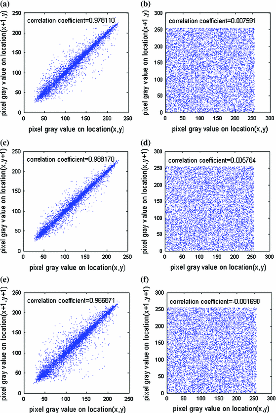
Correlations of two adjacent pixels in a horizontal direction of the plain-image, b horizontal direction of the cipher-image, c vertical direction of the plain-image, d vertical direction of the cipher-image, e diagonal direction of the plain-image, f diagonal direction of the cipher-image


A secure encryption scheme should remove the correlation between adjacent image pixels in order to improve the resistance against statistical analysis. To test the correlation between two adjacent pixels in vertical, horizontal and diagonal directions of a cipher-image, respectively, the following procedures are carried out. First, randomly select 10,000 pairs of two adjacent image pixels in the corresponding direction. Then, calculate the correlation coefficient of each pair using the following formula:
where \(x\) and \(y\) are grayscale values of two adjacent pixels in the image, \(E\left( x \right) =\frac{1}{N}\sum \nolimits _{i=1}^N {x_i } \hbox { and } D\left( x \right) =\frac{1}{N}\sum _{i=1}^N {\left( {x_i -E\left( x \right) } \right) ^{2}} \). In each test, \(N=10{,}000\). The correlation distributions of two adjacent pixels in the plain-image and the cipher-image are shown in Fig. 8, respectively. The measured correlation coefficients of the plain-image are close to 1, while those of the cipher-image are nearly 0. This indicates that the proposed algorithm has successfully removed the correlation of adjacent pixels in the plain-image so that neighbor pixels in the cipher-image virtually have no correlation. Therefore, the proposed algorithm possesses high security against statistical attacks.
4.5 Information entropy analysis
Information entropy, such as K–S, is the most outstanding feature of the randomness. It is well known that the entropy \(H(s)\) of a message source \(s\) can be measured by
where M is the total number of symbols \(s_{i}{\in s}, P(s_{i})\) represents the probability of occurrence of symbol \(s_{i}\). For a truly random source emitting 256 symbols, the ideal entropy is \(H(s) = 8\). If the output of a cipher emits symbols with the entropy value of less than 8, there is a certain degree of predictability which threatens its security. \(H(s)\) has been tested on the encrypted images. The results are shown in Table 3. Experiments results show that the cipher-images are close to a true random source and the proposed algorithm is secure against the entropy attack.
4.6 Resistance to known-plaintext and chosen-plaintext attacks
To resist the known-plaintext and chosen-plaintext attacks, two different plain-images should have different keystreams even if they are encrypted with identical keys. In the proposed algorithm, the status values of two tent maps are exchanged according to the previous pixel cipher value. Consequently, the next state value of maps is related to the plain-image. Since the pseudorandom number \({\varphi }(i)\), which is the keystream of the proposed algorithm, is related to the state values of maps, different images will have different \({\varphi }(i)\). It is difficult to decrypt a particular cipher-image using the keystream \({\varphi }(i)\) obtained from other images. Therefore, the proposed algorithm can well resist the known- plaintext and chosen-plaintext attacks.
4.7 Speed analysis
With the exception of security consideration, other issues of an image cryptosystem such as the operation speed are also significant, especially for real-time applications. The actual execution time of an algorithm is determined by many factors such as algorithm, programming skill, programming language and execution environment. Therefore, we discuss mainly the performance of the proposed scheme from the computational complexity perspective. The running speed of an algorithm based on chaotic maps is mainly determined by the following three factors:
-
(1)
Architecture of encryption/decryption.
-
(2)
Encryption rounds of algorithm.
-
(3)
Generating means of pseudorandom sequences.
To architecture of encryption/decryption, the permutation and diffusion processes are combined in the proposed algorithm, so only one time image-scanning step is required in each encryption round. This leads to a speed advantage compared with algorithms separating permutation and diffusion operations.
As shown in Table 4, the proposed cryptosystem and the Wang’s [xx] only need a minimum of two overall rounds to achieve a high performance such as \(\hbox {NPCR} > 0.996\) and \(\hbox {UACI} > 0.333\) for a tiny change at any position of the plain-image. The results show that the round number of encryption required by the proposed scheme is fewer than that by Wong’s and Lian’s. Thus, the proposed algorithm indeed leads to a faster encryption speed.
To generating pseudorandom sequences, the algorithms of Wong’s and Lian’s extract bits to generate pseudorandom numbers directly from the each iteration values of the logistic map and mask the image pixels one by one. In Wang’s algorithm, 8 times extracting operation are required per \(8\times 8\) block. Because the state value of a chaotic map is a floating-point number, and a pseudorandom number is usually an integer, the conversion from floating points to integers cannot be avoided in practical applications. Computer simulation results show that such a conversion is time-consuming [5]. Thus multiplication and conversion from floating points to integers should be avoided in order to have high efficiency of generating pseudorandom numbers. In our algorithm, only two times conversion is required per round as in Sect. 2.2 and Table 4, so the conversion from floating points to integers is avoided. Therefore, compared with these algorithms, our algorithm has faster running speed.
5 Conclusion
A fast and secure image encryption is proposed and analyzed. This employs two technologies to improve the encryption/decryption speed. One is to combine the permutation and diffusion stages. As a result, the image needs to be scanned only once in each encryption round. Another is an effective generation of pseudorandom numbers by S-Box lookup, XOR, Modular and cyclic shift operations and so on. It avoids some time-consuming operations such as bit extraction form floating-points and conversion from floating-points to integers, so a higher encryption speed is obtained. Then, both theoretical analyses and experimental tests have been carried out. The results show that satisfactory security performance is achieved in only two overall encryption rounds and so the speed efficiency is improved. Moreover, the security of the proposed scheme is verified by the analyses on its size of key space, key sensitivity, statistical and differential properties and so on. In conclusion, the new cipher indeed has excellent potential for practical image encryption applications.
References
Pisarchik, A.N., Zanin, M.: Image encryption with chaotically coupled chaotic maps. Phys. D 237, 2638–2648 (2008)
Fridrich, J.: Symmetric ciphers based on two-dimensional chaotic maps. Int. J. Bifurc. Chaos 8(6), 1259–1284 (1998)
Lian, S., Sun, J., Wang, Z.: A block cipher based on a suitable use of the chaotic standard map. Chaos Solitons Fractals 26, 117–129 (2005)
Wong, K.W., Kwok, B.S., Law, W.S.: A fast image encryption scheme based on chaotic standard map. Phys. Lett. A 372, 2645–2652 (2008)
Wang, Y., Wong, K.-W., Liao, X., Chen, G.: A new chaos-based fast image encryption algorithm. Appl. Soft Comput. 11, 514–522 (2011)
Yang, H., Wong, K.-W., Liao, X., Zhang, W., Wei, P.: A fast image encryption and authentication scheme based on chaotic maps. Commun. Nonlinear Sci. Numer. Simul. 15, 3507–3517 (2010)
Wang, Y., Liao, X., Xiao, D., Wong, K.-W.: One-way hash function construction based on 2D coupled map lattices. Inf. Sci. 178, 1391–1406 (2008)
Shannon, C.E.: Communication theory of secrecy system. Bell Syst. Tech. J. 28, 656–715 (1949)
Li, D., Hu, G.: A keyed hash function based on the modified coupled chaotic map lattice. Commun. Nonlinear Sci. Numer. Simul. 17, 2579–2587 (2012)
Yuen, C.-H., Wong, K.-W.: A chaos-based joint image compression and encryption scheme using DCT and SHA-1. Appl. Soft Comput. 11, 5092–5098 (2011)
Mohammad Seyedzadeh, S., Mirzakuchaki, S.: A fast color image encryption algorithm based on coupled two-dimensional piecewise chaotic map. Signal Process. 92, 1202–1215 (2012)
Pisarchik, A.N., Zanin, M.: Image encryption with chaotically coupled chaoticmaps. Phys. D 237, 2638–2648 (2008)
Xiang, T., Wong, K.W., Liao, X.: Selective image encryption using a spatiotemporal chaotic system. Chaos 17, 0231151–02311512 (2007)
Wang, X., Qin, X.: A new pseudo-random number generator based on CML and chaotic iteration. Nonlinear Dyn. 70, 1589–1592 (2012)
Liu, N., Guo, D., Parr, G.: Complexity of chaotic binary sequence and precision of its numerical simulation. Nonlinear Dyn. 67, 549–556 (2012)
Wei, J., Liao, X., Wong, K.W., Zhou, T.: Cryptanalysis of a cryptosystem using multiple one-dimensional chaotic maps. Commun. Nonlinear Sci. Numer. Simul. 12, 814–822 (2007)
Wang, K., Pei, W., Zou, L., Song, A., He, Z.: On the security of 3D cat map based symmetric image encryption scheme. Phys. Lett. A 343, 432–439 (2005)
Deng, S., Li, Y., Xiao, D.: Analysis and improvement of a chaos-based hash function construction. Commun. Nonlinear Sci. Numer. Simul. 15(5), 1338–1347 (2010)
Wang, S., Shan, P.: Security analysis of a one-way hash function based on spatiotemporal chaos. Chin. Phys. B 20, 090504–090507 (2011)
Kanso, A., Smaoui, N.: Irregularly decimated chaotic map(s) for binary digits generations. Int. J. Bifurcat. Chaos 19(4), 1169–1183 (2009)
Zhang, Y., Xiao, D., Wen, W., Nan, H.: Cryptanalysis of image scrambling based on chaotic sequences and Vigenère cipher. Nonlinear Dyn. (2014). doi:10.1007/s11071-014-1435-9
Zhang, Y., Xiao, D.: Cryptanalysis of S-box-only chaotic image ciphers against chosen plaintext attack. Nonlinear Dyn. 72(4), 751–756 (2013)
Yi, X., Tan, C.H., Siew, C.K.: A new block cipher based on chaotic tent maps. IEEE Trans. Circuits Syst. I 49(12), 1826–1829 (2002)
Jakimoski, G., Kocarev, L.: Chaos and cryptography: block encryption ciphers based on chaotic maps. IEEE Trans. Circuits Syst. I 48(2), 163–169 (2001)
Stojanovski, T., Kocarev, L.: Chaos-based random number generators-part I: analysis. IEEE Trans. Circuits Syst. I 48(3), 281–288 (2001)
Stojanovski, T., Kocarev, L.: Chaos-based random number generators-part II: practical realization. IEEE Trans. Circuits Syst. I 48(3), 382–385 (2001)
NIST Special Publication 800–22rev1a. http://csrc.nist.gov/groups/ST/toolkit/rng/index.html
Acknowledgments
Our sincere thanks go to the anonymous reviewers for their valuable comments. The work described in this paper was supported by the grants from the National Natural Science Foundation of China (No. 61003256), the Postdoctoral Science Foundation of China (2011M501391, 20110490082), the Natural Science Foundation of CQ CSTC (No. 2010BB2279) and the Program for excellent talents in Chongqing.
Author information
Authors and Affiliations
Corresponding author
Rights and permissions
About this article

Cite this article
Cheng, P., Yang, H., Wei, P. et al. A fast image encryption algorithm based on chaotic map and lookup table. Nonlinear Dyn 79, 2121–2131 (2015). https://doi.org/10.1007/s11071-014-1798-y
Received:
Accepted:
Published:
Issue Date:
DOI: https://doi.org/10.1007/s11071-014-1798-y