Hopf bifurcation in delayed van der Pol oscillators

Abstract

In this paper, we consider a classical van der Pol equation with a general delayed feedback. Firstly, by analyzing the associated characteristic equation, we derive a set of parameter values where the Hopf bifurcation occurs. Secondly, in the case of the standard Hopf bifurcation, the stability of bifurcating periodic solutions and bifurcation direction are determined by applying the normal form theorem and the center manifold theorem. Finally, a generalized Hopf bifurcation corresponding to non-semisimple double imaginary eigenvalues (case of 1:1 resonance) is analyzed by using a normal form approach.

1 Introduction

The van der Pol oscillator is an oscillator with nonlinear damping governed by the second-order differential equation

$$ \ddot{x}-\varepsilon\bigl(1-x^2\bigr)\dot{x}+x=0. $$

(1)

This model was originally proposed by Balthasar van der Pol [1]. The van der Pol equation, which was later extensively studied as a host of a rich class of dynamical behavior, including relaxation oscillations, quasi-periodicity, elementary bifurcations and chaos, plays an important role in electronics and mathematics dynamical systems.

Recently, the van der Pol equations with time delay have been studied by many researchers. Atay [2] has studied the behavior of the limit cycle of the van der Pol equations of the following forms:

$$ \ddot{x}-\varepsilon\bigl(1-x^2\bigr)\dot{x}+x= \varepsilon kx(t-\tau) $$

(2)

and

$$ \ddot{x}-\varepsilon\bigl(1-x^2\bigr)x(t-\tau)+x=0. $$

(3)

Meanwhile, it has been shown how the presence of delay can change the amplitude of limit oscillations, or suppress them altogether. Wei & Jiang [3] have found that there are stability switches when the delay varies and the above systems undergo a Hopf bifurcation at the origin when τ passes through a sequence of critical values. Moreover, using the normal form theory and the center manifold theorem, the stability of the bifurcating periodic solutions and the direction of the Hopf bifurcation are determined. Furthermore, Jiang & Wei [4] considered the following van der Pol equation with delayed feedback:

$$ \ddot{x}-\varepsilon\bigl(1-x^2\bigr)\dot{x}+x= \varepsilon g\bigl(x(t-\tau)\bigr), $$

(4)

where

$$g(0)=0,\quad g'(0)=k\neq0, $$

and showed that there were Bogdanov–Takens bifurcation, triple zero, and Hopf-zero singularities for the system under certain conditions. As shall be seen, the non-semisimple 1:1 resonance case in which the characteristic equation of either (2) or (4) has two equal nonzero imaginary roots has not been studied and this case arises very naturally. Surprisingly, this phenomena has not been discovered in the literatures.

In this paper, we consider the following van der Pol equation with delayed feedback, including Eqs. (2) and (4) as special cases,

$$ \ddot{ x}-\varepsilon\bigl(1-x^2\bigr)\dot{x}+x=f \bigl(x(t-\tau)\bigr), $$

(5)

where x is a dynamical variable and the forcing f(x(t−τ)) is a delayed feedback of the position x. Throughout this paper, we always assume that function f: ℝ→ℝ satisfies

$$ \everymath{\displaystyle} \begin{array}{@{}l} f(0)=f''(0)=0, \qquad f'(0)=\gamma, \quad\mbox{and} \\[2mm] f'''(0)= \delta. \end{array} $$

(6)

We see that system (5) undergoes a Hopf bifurcation at the origin when (ε,τ,γ) passes through a critical set. Our motivation is two-fold. First of all, we unify and improve the existing results in reference [3]. The other reason is that we want to obtain explicit expressions in terms of the coefficients of the original systems that determine whether either no branch, or one, or two branches of periodic solutions exist as the parameter (ε,τ,γ) varies.

In Sect. 2, we establish a set $\mathcal{H}$ of parameter values at which Hopf bifurcation of the equilibrium solution x=0 of (5) occurs. In Sect. 3, we perform a center manifold reduction and normal form approach on (5), obtaining formulae determining the Hopf direction and stability of bifurcating periodic solutions when the eigenvalues of the infinitesimal generator associated with the linearization equation of (5) at the zero solution are a pair of simple purely imaginary complex number at the critical parameter $(\varepsilon,\tau,\gamma)\in\mathcal{H}$.

As we shall see in Sect. 2, at some points of the Hopf bifurcation surface $\mathcal{H}$, the infinitesimal generator has a pair of double purely imaginary eigenvalues, which are non-semisimple, i.e., their geometric multiplicities not equal to their algebraic multiplicities. Surprisingly, this phenomena has not been discovered in delayed van der Pol equation (5). In Sect. 4, a center manifold combined with normal formal analysis is used to predict a set of ordinary differential equations approximating the flow of the full equation near these nonsemisimple 1:1 resonant Hopf bifurcation points. This, together with the works by van Gils et al. [5], implies that Eq. (5) may have 0, 1, or 2 periodic orbits near these non-semisimple 1:1 resonant Hopf bifurcation points. In Sect. 5, we show numerical simulations of Eq. (5) for parameter values in the neighborhood of the critical point of Sect. 3.

2 Hopf bifurcation analysis

In this section, we shall investigate the occurrence of Hopf bifurcation and the stability of the zero solution.

The characteristic equation of the linearization of (5) about the equilibrium point x=0 is

$$ \lambda^2-\varepsilon\lambda+1=\gamma e^{-\lambda\tau}. $$

(7)

First, we know that ±iω (ω>0) are a pair of purely imaginary roots of (7) if and only if ω satisfies

$$ \left\{ \begin{array}{l} 1-\omega^2=\gamma\cos\tau\omega, \\ \varepsilon\omega=\gamma\sin\tau\omega. \end{array} \right. $$

(8)

Hence, the Hopf bifurcation surface is given by

Then it follows from (8) that ω satisfies

$$ \frac{\varepsilon\omega}{1-\omega^2}=\tan\tau \omega. $$

(9)

Next, we consider the simplicity of ±iω. If iω is not simple, then we have

$$\frac{\mathrm{d}}{\mathrm{d}\lambda}\bigl(\lambda^2-\varepsilon \lambda+1-\gamma \mathrm{e}^{-\lambda\tau}\bigr) \big|_{\lambda=\mathrm{i}\omega }=0, $$

that is

$$\bigl(2\lambda-\varepsilon+\tau\gamma\mathrm{e}^{-\lambda\tau }\bigr) \big|_{\lambda =\mathrm{i}\omega}=0, $$

i.e.,

$$2\mathrm{i}\omega-\varepsilon+\tau\gamma(\cos\omega\tau-\mathrm {i}\sin \omega\tau)=0. $$

Separating the real and imaginary parts, we obtain

$$ \begin{array}{@{}l} \varepsilon=\tau\gamma\cos\omega\tau, \\[1mm] 2\omega=\tau\gamma\sin\omega\tau. \end{array} $$

(10)

It follows from (8) and (10) that

$$ \begin{array}{@{}l} \tau\varepsilon=2, \\[1mm] \tau\bigl(1-\omega^2\bigr)=\varepsilon, \\[1mm] \tau\omega=\xi, \end{array} $$

(11)

where x=ξ>0 is a solution to the equation x=tanx. Then it follows from (11) that

$$ \everymath{\displaystyle} \begin{array}{@{}l} \tau=\sqrt{2+\xi^2}, \\[4.5mm] \varepsilon=\frac{2}{\sqrt{2+\xi^2}}, \\[5mm] \omega=\frac{\xi}{\sqrt{2+\xi^2}}. \end{array} $$

(12)

Let $\{\xi_{n}\}^{\infty}_{n=1}$ be the monotonic increasing sequence of the positive solutions of x=tanx, and

$$ \everymath{\displaystyle} \begin{array}{@{}l} \tau_n^*=\sqrt{2+\xi_n^2}, \qquad\varepsilon _n^*=\frac{2}{\sqrt{2+\xi_n^2}}, \\[5mm] \omega_n^*=\frac{\xi_n}{\sqrt{2+\xi_n^2}}, \qquad\gamma_n^*=\frac {2\xi_n}{(2+\xi_n^2)\sin\xi_n}. \end{array} $$

(13)

Then we have the following results.

Lemma 1

At and only at $(\varepsilon,\tau,\gamma )\in\mathcal{H}\backslash\{(\varepsilon_{n}^{*},\tau_{n}^{*},\allowbreak \gamma_{n}^{*})\} ^{\infty}_{n=1}$, Eq. (7) has a pair of simple purely imaginary solutions ±iω, where ω is a solution to (8). Moreover, at and only at $(\varepsilon ,\tau ,\gamma)=(\varepsilon^{*}_{n},\tau^{*}_{n},\gamma^{*}_{n})$ for some n∈ℕ⁺, Eq. (7) has a pair of double purely imaginary solutions $\pm\mathrm{i}\omega^{*}_{n}$.

Now we consider what happen to the solutions of Eq. (7) as the point (ε,τ,γ) passes through the Hopf bifurcation surface $\mathcal{H}$. We start with the case where $(\varepsilon_{0},\tau_{0},\gamma_{0})\in\mathcal {H}\backslash\{(\varepsilon_{n}^{*},\tau_{n}^{*},\gamma_{n}^{*})\}^{\infty}_{n=1}$. By the implicit function theorem, there exist a neighborhood N(ε ₀,τ ₀,γ ₀) and a mapping λ:N(ε ₀,τ ₀,γ ₀)→ℂ such that λ(ε ₀,τ ₀,γ ₀)=λ ₀=iω ₀, and for each (ε,τ,γ)∈N(ε ₀,τ ₀,γ ₀), λ(ε,τ,γ) is always the solution to (7), where ω ₀>0 satisfies $\frac{\varepsilon_{0}\omega_{0}}{1-\omega _{0}^{2}}=\tan\tau_{0}\omega_{0}$.

Using the implicit differentiation, we have

where

$$\varDelta=(\tau_0\gamma_0\cos\omega_0 \tau_0-\varepsilon_0)^2+(2 \omega_0-\tau_0\gamma_0\sin \omega_0\tau_0)^2. $$

Thus, we have

Then we can summarize the above discussion as follows.

Lemma 2

Suppose that $(\varepsilon_{0},\tau_{0},\gamma_{0})\in \mathcal {H}\backslash\{(\varepsilon_{n}^{*},\tau_{n}^{*},\allowbreak \gamma_{n}^{*})\}^{\infty}_{n=1}$, then

• (i) Fixing (τ,γ)=(τ ₀,γ ₀) and regarding ε as a bifurcation parameter, suppose that ε ₀ τ ₀≠2 (i.e., the transversality condition holds), then system (5) undergoes a Hopf bifurcation at the origin when ε=ε ₀.

• (ii) Fixing (ε,γ)=(ε ₀,γ ₀) and regarding τ as a bifurcation parameter, suppose that $2\omega_{0}^{2}+\varepsilon_{0}^{2}-2\neq\nobreak 0$ (i.e., the transversality condition holds), then system (5) undergoes a Hopf bifurcation at the origin when τ=τ ₀.

• (iii) Fixing (ε,τ)=(ε ₀,τ ₀) and regarding γ as a bifurcation parameter, suppose that $\tau _{0}\gamma_{0}^{2}-\varepsilon_{0}(1+\nobreak \omega_{0}^{2})\neq0$ (i.e., the transversality condition holds), then system (5) undergoes a Hopf bifurcation at the origin when γ=γ ₀.

Finally, we consider the stability of the zero solution. Wei & Jiang [3] have investigated the stability of the zero solution by regarding τ as a bifurcation parameter. Hence, in the sequel, we will fix (ε,τ) and regard γ as a parameter. Firstly, using a similar argument to that in [6], we have the following result.

Lemma 3

For each fixed $(\varepsilon,\tau)\notin\{ (\varepsilon_{n}^{*},\tau_{n}^{*}): n\in\mathbb{N}\}$, there exists a sequence {γ _j } _{j∈ℤ∖{0}} satisfying ⋯<γ _−j <⋯<γ ₋₁<0<γ ₁<⋯<γ _j <⋯, such that Eq. (7) with γ=γ _j has a simple pair of purely imaginary roots ±iω _j , where ω _j is a positive solution of Eq. (9) and $\gamma_{j}=\frac{\varepsilon\omega_{j}}{\sin \omega_{j}\tau}$.

Now we consider the case where the characteristic equation of system (5) has zero solution. Clearly, Eq. (7) is the same as that of Eq. (4) with εk replaced by γ. So, we obtain the following results similar to that in [4].

Lemma 4

Suppose that γ=1 is satisfied. Then

• (i) λ=0 is a simple solution to Eq. (7) when τ≠ε;

• (ii) λ=0 is a double solution to Eq. (7) when $\tau=\varepsilon\neq\sqrt{2}$;

• (iii) λ=0 is a triple solution to Eq. (7) when $\tau=\varepsilon=\sqrt{2}$;

• (iv) there exists a sequence $\{\tau_{j}\}_{j=0}^{\infty}$ satisfying τ _j+1>τ _j such that Eq. (7) with τ=τ _j has a pair of purely imaginary roots $\pm\mathrm{i}\bar {\omega }$, where $\bar{\omega}=\sqrt{2-\varepsilon^{2}}$, and

  $$\tau_j=\left\{ \begin{array}{l} \frac{1}{\bar{\omega}}(\arcsin\varepsilon\bar {\omega}+2j\pi), \quad1<\varepsilon<\sqrt{2}, \\[1mm] \frac{1}{\bar{\omega}}(\pi-\arcsin\varepsilon\bar{\omega}+2j\pi ), \\ \quad0<\varepsilon\leq1,\ j=0,1,\ldots. \end{array} \right. $$

Theorem 1

For system (5), γ=1+μ is regarded as a bifurcation parameter.

• (i) If γ=1 and 0<τ<ε, then Eq.(7) has at least one positive real root, so the zero solution of system (5) is unstable.

• (ii) If ε<τ<τ ₀ and $0<\varepsilon<\sqrt {2}$, then system (5) undergoes a pitchfork bifurcation at the origin when μ=0.

• (iii) If τ=ε and $0<\varepsilon<\sqrt{2}$, then system (5) undergoes a Bogdanov–Takens bifurcation at the origin when μ=0.

• (iv) If τ=τ ₀≠ε and $0<\varepsilon <\sqrt{2}$, then system (5) undergoes a Hopf-zero bifurcation at the origin when μ=0.

• (v) If $\tau=\varepsilon=\sqrt{2}$, then system (5) undergoes a triple zero bifurcation at the origin when μ=0.

Theorem 2

Suppose that ε<τ<τ ₀ and $0<\varepsilon<\sqrt{2}$. Then

• (i) The zero solution of (5) with γ=1 is asymptotically stable (respectively, unstable) when δ<0 (respectively, >0).

• (ii) For system (5) with γ=1+μ, μ∈ℝ is sufficiently small. Then the zero solution is asymptotically stable when μ<0 and unstable when μ>0.

The proofs of Theorems 1–2 are similar to that in [4], and hence are omitted.

Here, we will only consider the case where τ≠ε and Eq. (13) is not valid for (ε,τ). According to Lemmas 3 and 4, the characteristic eigenvalues with $\operatorname{Re}\lambda=0$ of Eq. (5) are all simple. By Rouché’s theorem [7], as γ varies the sum of the multiplicities of the roots of Eq. (7) in the open right half-plane can change only if a root appears on, or crosses the imaginary axis.

Note that when γ=0, Eq. (7) becomes

$$ \lambda^2-\varepsilon\lambda+1=0, $$

(14)

whose roots are $\lambda_{1,2}=\frac{1}{2}(\varepsilon\pm\sqrt {\varepsilon^{2}-4})$. Clearly, there are two roots λ _1,2 satisfying $\operatorname{Re}\lambda_{1,2}>0$. It is easy to see that the stability of zero solution can change a finite number of times, at most, and eventually it becomes unstable as γ is increased from γ ₁ to infinity (or decreased from γ ₋₁ to infinity). In a summary, we have the following results.

Theorem 3

Suppose that ε≠τ, Eq. (13) is not valid for (ε,τ) and the transversality condition $\operatorname{Re}\lambda'_{\gamma}(\varepsilon,\tau,\allowbreak \gamma_{j})\neq0$ for each γ _j ∈{γ _j } _{j∈ℤ∖{0}}. Then we have the following information about the stability of the zero solution.

• (i) If γ∈(γ ₋₁,min{1,γ ₁}), the instability degree of system (5) (the multiplicity of roots with positive real parts of Eq.(7)) equals to two, then the zero solution of system (5) is unstable.

• (ii) When γ increases and passes through γ _j (γ _j ≠1), the instability degree of system (5) increases (respectively, decreases) by two if $\operatorname {Re}\lambda'_{\gamma}(\varepsilon,\tau,\gamma_{j})>\nobreak 0$ (respectively, <0).

• (iii) If 0<τ<ε and $\tau\notin\{\tau_{j}\} _{j=0}^{\infty}$ (defined in Lemma 4), then Eq. (7) with γ=1 has a simple zero solution and there exists an integer i∈ℕ, such that 1∈(γ _i ,γ _i+1), where γ ₀=0. For each γ∈(γ _i ,γ _i+1), Eq. (7) has at least one positive real root, i.e., the zero solution of system (5) is unstable. Moreover, the instability degree of system (5) decreases by 1 when γ increases and passes through 1.

• (iv) If 0<τ<ε and $\tau\in\{\tau_{j}\} _{j=0}^{\infty}$, then Eq. (7) with γ=1 has a simple zero solution and a pair of simple imaginary roots $\pm\mathrm{i}\bar {\omega}$, and there exists an integer i∈ℕ⁺, such that γ _i =1. Similarly, for all γ∈(γ _i−1,γ _i+1), Eq. (7) has at least one positive real root, i.e., the zero solution of system (5) is unstable. Moreover, the instability degree of system (5) increases by 1 if $\operatorname{Re}\lambda'_{\gamma}(\varepsilon,\tau,1)>0$ or decreases by 3 if $\operatorname{Re}\lambda'_{\gamma}(\varepsilon,\tau,1)<0$ when γ increases and passes through 1.

• (v) If 0<ε<τ<τ ₀, then Eq. (7) with γ=1 has a simple zero solution and there exists an integer i∈ℕ, such that 1∈(γ _i ,γ _i+1). The instability degree of system (5) increases by 1 when γ increases and passes through 1. Furthermore, suppose that $0<\varepsilon<\sqrt{2}$, the zero solution of system (5) with γ=1 is asymptotically stable (respectively, unstable) when δ<0 (respectively, >0); the zero solution of system (5) with γ∈(γ _i ,1) (respectively, γ∈(1,γ _i+1)) is asymptotically stable (respectively, unstable).

• (vi) If 0<ε<τ, $\tau\in\{\tau_{j}\} _{j=0}^{\infty}$ and $0<\varepsilon<\sqrt{2}$, then Eq. (7) with γ=1 has a simple zero solution and a pair of simple imaginary roots $\pm\mathrm{i}\bar{\omega}$. There exists an integer i∈ℕ⁺, such that γ _i =1. As γ increases and passes through 1, the instability degree of system (5) increases by 3 if $\operatorname{Re}\lambda '_{\gamma}(\varepsilon,\tau,1)>0$ or decreases by 1 if $\operatorname {Re}\lambda'_{\gamma}(\varepsilon,\tau,1)<0$.

• (vii) If 0<ε<τ and $\tau\notin\{\tau_{j}\} _{j=0}^{\infty}$, or 0<ε<τ and $\varepsilon>\sqrt{2}$, then Eq. (7) with γ=1 has a simple zero solution and there exists an integer i∈ℕ, such that 1∈(γ _i ,γ _i+1). The instability degree of system (5) increases by 1 when γ increases and passes through 1.

• (viii) There exists an integer m≥1, such that for all γ>γ _m or γ<γ _−m , the zero solution of system (5) is unstable.

3 Direction and stability of Hopf bifurcation at simple eigenvalues

Let $\dot{x}(t)=y(t)$, then Eq. (5) becomes

$$ \begin{array} {@{}l} \dot{x}(t)=y(t), \\[2mm] \dot{y}(t)=-x(t)+\varepsilon\bigl(1-x^2(t)\bigr)y(t)+f\bigl(x(t- \tau)\bigr). \end{array} $$

(15)

Assume that system (5) undergoes a Hopf bifurcation at the origin when (ε,τ,γ)=(ε ₀,τ ₀,γ ₀) and the corresponding characteristic equation has a pair of simple imaginary roots ±iω ₀.

Firstly, we rescale the time by $t\rightarrow\frac{t}{\tau}$ to normalize the delay, then the above system becomes

$$ \begin{array} {@{}rcl} \dot{x}(t)&=&\tau y(t), \\[2mm] \dot{y}(t)&=&-\tau x(t)+\varepsilon\tau\bigl(1-x^2(t)\bigr)y(t) \\[2mm] &&{}+\tau f \bigl(x(t-1)\bigr). \end{array} $$

(16)

For convenience, set μ=(ε,τ,γ)−(ε ₀,τ ₀,γ ₀), where μ∈ℝ³. Then μ=0 is the Hopf bifurcation value for system (16), and the corresponding eigenvalues are ±iτ ₀ ω ₀.

As usual, the phase space C=C([−1,0],ℝ²) is the Banach space of continuous functions from [−1,0] to ℝ² with the supremum norm ∥ϕ∥=sup_{−1≤θ≤0}|ϕ(θ)| for ϕ∈C. For φ∈C, let

$$ L_\mu\varphi=\tau\mathbf{B}_1\varphi(0)+\tau\gamma \mathbf{B}_2\varphi(-1), $$

(17)

where

$$\mathbf{B}_1=\left( \begin{array}{c@{\quad}c} 0 & 1\\ -1 & \varepsilon \end{array} \right) \quad\mbox{and} \quad\mathbf{B}_2=\left( \begin{array}{c@{\quad}c} 0 & 0\\ 1 & 0 \end{array} \right), $$

and

By the Riesz representation theorem, there exists a 2×2 matrix-valued function η(θ,μ):[−1,0]×ℝ³→ℝ⁴, whose elements are bounded variation functions, such that

$$L_\mu\varphi=\int^0_{-1}\mathrm{d}\eta( \theta,\mu)\varphi(\theta), \quad\varphi\in C. $$

In fact, we can choose

$$\eta(\theta,\mu)=\left\{ \begin{array}{l@{\quad}l} \tau\mathbf{B}_1, \qquad& \theta=0, \\ -\tau\gamma\mathbf{B}_2\delta(\theta+1),\quad& \theta\in[-1,0), \end{array} \right. $$

where δ(θ) is the Dirac delta function. Next, we define for φ∈C ¹([−1,0],ℝ²)

$$\mathcal{A}(\mu)\varphi=\left\{ \begin{array}{l@{\quad}l} \frac{\mathrm{d}\varphi(\theta)}{\mathrm {d}\theta}, & \theta\in[-1,0), \\[1mm] L_\mu\varphi, & \theta=0 \end{array} \right. $$

and

$$\mathbf{X}_0=\left\{ \begin{array}{l@{\quad}l} \mathbf{I}_2,& \theta=0, \\ 0,& \theta\in[-1,0), \end{array} \right. $$

where I _n is n-order identity matrix. Then we can rewrite Eq. (16) as

$$ \dot{\mathbf{u}_t}=\mathcal{A}(\mu) \mathbf{u}_t+\mathbf{X}_0\mathbf{F}(\mu, \mathbf{u}_t), $$

(18)

where u=(u ₁,u ₂)^T,u _t =u(t+θ) for θ∈[−1,0].

For ψ∈C ¹([0,1],ℝ^2∗), define

$$\mathcal{A}^*\psi(s)=\left\{ \begin{array}{l@{\quad}l} -\frac{\mathrm{d}\psi(s)}{\mathrm{d}s}, & s\in(0,1], \\[1mm] \int^0_{-1}\psi(-s)\,\mathrm{d}\eta(s,0), & s=0. \end{array} \right. $$

Then, for φ∈C, and ψ∈C ¹([0,1],ℝ^2∗), define the bilinear form

(19)

It is easy to check that $\mathcal{A^{*}}$ and $\mathcal{A}(0)$ are adjoint operators, and ±iτ ₀ ω ₀ are eigenvalues of $\mathcal{A}(0)$. Thus, they are also eigenvalues of $\mathcal{A^{*}}$. By direct computation, we obtain the following lemma.

Lemma 5

${\mathbf{q}(\theta)=(1,\mathrm{i}\omega_{0})^{T} \mathrm{e}^{\mathrm {i}\tau _{0}\omega_{0}\theta}}$ is the eigenvector of $\mathcal{A}(0)$ associated with iτ ₀ ω ₀; $\mathbf{p}(s)=D(\varepsilon _{0}+\mathrm{i}\omega_{0},-1)\mathrm{e}^{\mathrm{i}\tau_{0}\omega_{0}s}$ is the eigenvector of $\mathcal{A^{*}}$ associated with −iτ ₀ ω ₀, where $D=(\varepsilon_{0}+2\mathrm{i}\omega_{0}-\gamma_{0}\tau_{0} \mathrm {e}^{\mathrm{i}\tau _{0}\omega_{0}})^{-1}$. Moreover, 〈p,q〉=1, and $\langle\mathbf{p},\bar{\mathbf{q}}\rangle=0$.

Let $\boldsymbol{\Psi}=(\mathbf{p},\overline{\mathbf{p}})$ and $\boldsymbol{\Phi}=(\mathbf {q},\overline{\mathbf{q}})$. By the center manifold theorem, we obtain the reduced equation

$$ \dot{z}={\mathrm{i}}\tau_0\omega_0z+g(\mu,z,\bar{z}), $$

(20)

where $g(\mu,z,\bar{z})=\overline{\mathbf{p}}(0)\mathbf{F}(\mu,2 \operatorname{Re}\{z(t)\mathbf{q}(\theta)\}+\mathbf{w}(\mu,\allowbreak z,\bar {z}))$ and $\mathbf{w}(\mu,z,\bar{z})$ satisfies that

$$ \dot{\mathbf{w}}=\mathcal{A}\mathbf{w}+\mathbf{H}(z,\bar {z},\theta) $$

(21)

with $\mathbf{H}(z,\bar{z},\theta)=[\mathbf{X}_{0}-\boldsymbol {\Phi}\boldsymbol{\Psi }(0)]\mathbf{F}(\mu,2\operatorname{Re}\{z(t)\mathbf{q}(\theta)\} +\mathbf {w}(\mu,z,\bar{z}))$. Let

and

$$ \mathbf{w}(t,\theta)=\mathbf{w}_{20}^\mu\frac{z^2}{2}+ \mathbf{w}_{11}^\mu z\bar{z}+\mathbf{w}_{02}^\mu \frac{\bar{z}^2}{2}+\cdots. $$

Using a computation process similar to that in [3], we obtain the coefficients used in determining the important quantities:

$$g_{20}^0=g_{11}^0=g_{02}^0=0, $$

and

$$g_{21}^0=\overline{D}\tau_0\bigl(2{\mathrm{i}} \varepsilon_0\omega_0-\delta\mathrm{{e}}^{-\mathrm{i}\omega_0\tau_0} \bigr). $$

Then from

$$C_1(0)=\frac{{\mathrm{i}}}{2\tau_0\omega_0}\biggl [g_{20}^0G_{11}^0 \,{-}\, 2\bigl|g_{11}^0\bigr|^2 \,{-}\, \frac{1}{3}\bigl|g_{11}^0\bigr|^2\biggr] \,{+}\, \frac{g_{21}^0}{2}, $$

we have

By the general theory of Hopf bifurcation, we have the following results:

Theorem 4

For any fixed $(\varepsilon_{0},\tau_{0},\gamma_{0})\in\mathcal {H}\backslash \{(\varepsilon_{n},\tau_{n},\allowbreak \gamma_{n})\}^{\infty}_{n=1}$ with the corresponding eigenvalues ±iω ₀ satisfying (7), we have

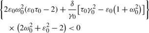
• (i) If (τ,γ)=(τ ₀,γ ₀), the Hopf bifurcation at the origin when ε=ε ₀ is supercritical (respectively, subcritical) when

  

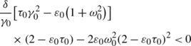
  (respectively, >0) and the bifurcating periodic solutions have the same stability as the trivial solution had before the bifurcation (respectively, are unstable) when $2\varepsilon _{0}\omega_{0}^{2}(\varepsilon_{0}\tau_{0}-2)+\frac{\delta}{\gamma_{0}}[\tau _{0}\gamma_{0}^{2}-\varepsilon_{0}(1+\omega_{0}^{2})]<0$ (respectively, >0).

• (ii) If (ε,γ)=(ε ₀,γ ₀), the Hopf bifurcation at the origin when τ=τ ₀ is supercritical (respectively, subcritical) when

  

  (respectively, >0) and the bifurcating periodic solutions have the same stability as the trivial solution had before the bifurcation (respectively, are unstable) when $2\varepsilon _{0}\omega_{0}^{2}(\varepsilon_{0}\tau_{0}-2)+\frac{\delta}{\gamma_{0}}[\tau _{0}\gamma_{0}^{2}-\varepsilon_{0}(1+\omega_{0}^{2})]<0$ (respectively, >0).

• (iii) If (ε,τ)=(ε ₀,τ ₀), the Hopf bifurcation at the origin when γ=γ ₀ is supercritical (respectively, subcritical) when

  

  (respectively, >0) and the bifurcating periodic solutions have the same stability as the trivial solution had before the bifurcation (respectively, are unstable) when $2\varepsilon _{0}\omega_{0}^{2}(\varepsilon_{0}\tau_{0}-2)+\frac{\delta}{\gamma_{0}}[\tau _{0}\gamma_{0}^{2}-\varepsilon_{0}(1+\omega_{0}^{2})]<0$ (respectively, >0).

In particular, if δ=0, then Eq. (5) becomes Eq. (2) with εk replaced by γ. Thus, we can obtain the following results.

Corollary 1

Assume that δ=0, and for any fixed $(\varepsilon_{0},\tau_{0},\gamma_{0})\in\mathcal{H}\backslash\{ (\varepsilon_{n},\tau_{n},\gamma_{n})\}^{\infty}_{n=1}$ with the corresponding eigenvalues ±iω ₀ satisfying (7), we have

• (i) The Hopf bifurcation at ε=ε ₀ is supercritical if ε ₀ τ ₀≠2 and the bifurcation periodic solutions have the same stability as the trivial solution had before the bifurcation (respectively, are unstable) if ε ₀ τ ₀<2 (respectively, >2).

• (ii) The Hopf bifurcation at τ=τ ₀ is supercritical (subcritical) when

  $$(\varepsilon_0\tau_0-2) \bigl(2\omega_0^2+ \varepsilon_0^2-2\bigr)<0 $$

  (respectively, >0) and the bifurcation periodic solutions have the same stability as the trivial solution had before the bifurcation (respectively, are unstable) if ε ₀ τ ₀<2 (respectively, >2).

• (iii) The Hopf bifurcation at γ=γ ₀ is supercritical (subcritical) when

  $$\gamma_0(\varepsilon_0\tau_0-2)\bigl[ \tau_0\gamma_0^2-\varepsilon_0 \bigl(1+\omega_0^2\bigr)\bigr]<0 $$

  (respectively, >0) and the bifurcation periodic solutions have the same stability as the trivial solution had before the bifurcation (respectively, are unstable) if ε ₀ τ ₀<2 (respectively, >2).

Remark

In [3], Wei & Jiang have found that there exists a sequence of critical points $\{\tau_{j}^{\pm}\}_{j=0}^{\infty}$ when the parameters ε and γ are restricted under certain conditions, and obtain the bifurcation direction and stability of the Hopf bifurcation. Their results are similar to Corollary 1(ii). Hence, Theorem 4 not only unifies but also improves the existing results.

4 Hopf bifurcation with non-semisimple 1:1 resonance

From the discussion given in Sect. 2, we know that the linearization of Eq. (5) has a pair of double purely imaginary eigenvalues ±iω ^∗ at (ε ^∗,τ ^∗,γ ^∗) satisfying (13). Then we can obtain a four-dimensional reduced equation on the center manifold.

Using the same notation as in Sect. 3, denote by P and P ^∗ as the generalized eigenspace of $\mathcal{A}(0)$ and $\mathcal{A}^{*}$ associated with the imaginary characteristic roots iτ ^∗ ω ^∗ and −iτ ^∗ ω ^∗, respectively. It is easy to see that dimP=dimP ^∗=4. Then we suppose that the bases of P and P ^∗, respectively, are

$$\boldsymbol{\Phi}(\theta)=\bigl(\mathbf{q}_1(\theta),\overline{ \mathbf{q}_1}(\theta),\mathbf{q}_2(\theta),\overline{ \mathbf{q}_2}(\theta)\bigr) $$

and

$$\boldsymbol{\Psi}(s)=\bigl(\mathbf{q}_1^*(s),\overline{ \mathbf{q}_1^*}(s),\mathbf{q}_2^*(s),\overline{ \mathbf{q}_2^*}(s)\bigr) $$

with

$$\bigl\langle\boldsymbol{\Phi}(s),\boldsymbol{\Psi}(\theta)\bigr \rangle={ \mathbf{I}}_4. $$

By direct computation, we have

and

where

$$\tilde{D}=\tau^*\biggl(\frac{1}{2}\gamma^*\tau^{*2}{ \mathrm{e}}^{{\mathrm{i}}\omega ^*\tau^*}-1\biggr)^{-1}. $$

We first compute the coordinates to describe the center manifold at (ε ^∗,τ ^∗,γ ^∗). Let u _t be the solution of Eq. (18), define

$$z_1(t)=\bigl\langle\mathbf{q}_1^*,\mathbf{u}_t \bigr\rangle, \qquad z_2(t)=\bigl\langle\mathbf{q}_2^*, \mathbf{u}_t\bigr\rangle, $$

and

$$\mathbf{w}(z_1,\bar{z_1},z_2, \bar{z_2})=\mathbf{u}_t-2\operatorname{Re}\{ z_1 \mathbf{q}_1\}-2\operatorname{Re}\{z_2\mathbf{q}_2\}. $$

Then, on the center manifold, we can obtain the reduced equation

$$ \everymath{\displaystyle} \begin{array}{@{}l} \dot{z_1}(t)={\mathrm{i}}\tau^*\omega ^*z_1+z_2+g^1(\mathbf{z},\bar{\mathbf{z}}), \\[1mm] \dot{z_2}(t)={\mathrm{i}}\tau^*\omega^*z_2+g^2(\mathbf{z},\bar {\mathbf{z}}), \end{array} $$

(22)

where z=(z ₁,z ₂)^T and

and

$$\mathbf{w}(\mathbf{z},\bar{\mathbf{z}})=\sum\limits _{j+s+k+r\geq2}\frac {1}{j!s!k!r!}\mathbf{w}_{jskr}z_1^j \bar{z_1}^sz_2^k \bar{z_2}^r $$

satisfies

(23)

Let

We know that (22) has the formal normal form

$$ \everymath{\displaystyle} \begin{array}{@{}l} \dot{z_1}={\mathrm{i}}\tau^*\omega ^*z_1+z_2+z_1\varphi_1(u_1,u_2),\\[1mm] \dot{z_2}={\mathrm{i}}\tau^*\omega^*z_2+z_2\varphi _1(u_1,u_2)+z_1\varphi_2(u_1,u_2), \end{array} $$

(24)

where u ₁=|z ₁|², $u_{2}=z_{1}\bar{z_{2}}-\bar{z_{1}}z_{2}$, and φ _j (j=1,2) are polynomials in their arguments such that φ _j (0,0)=0. Let

$$ \everymath{\displaystyle} \begin{array}{@{}l} \varphi_1(u_1,u_2)=a_1u_1+a_2u_2+O\bigl(\|z\|^4\bigr), \\[1mm] \varphi_2(u_1,u_2)=b_1u_1+b_2u_2+O\bigl(\|z\|^4\bigr), \end{array} $$

(25)

then (24) can be rewritten in the following form:

$$ \begin{array}{@{}ll} \dot{z_1}&={\mathrm{i}}\tau^*\omega^*z_1+z_2+a_1z_1^2\bar {z_1}+a_2z_1^2\bar {z_2}-a_2z_1\bar{z_1}z_2 \\[1mm] &\quad {}+O\bigl(\|z\|^4\bigr), \\[2mm] \dot{z_2}&={\mathrm{i}}\tau^*\omega^*z_2+b_1z_1^2\bar {z_1}+b_2z_1^2\bar {z_2}+(a_1-b_2)z_1\bar{z_1}z_2 \\[1mm] &\quad{}+a_2z_1z_2\bar{z_2}-a_2\bar{z_1}z_2^2+O\bigl(\|z\|^4\bigr). \end{array} $$

(26)

As in [8], we could rewrite (22) in the following form:

$$ \dot{\mathbf{y}}=\mathbf{A}\mathbf{y}+\mathbf {f}(\mathbf{y}), $$

(27)

where $\mathbf{y}=(z_{1},\bar{z}_{1},z_{2},\bar{z}_{2})^{T}$, f:ℂ⁴→ℂ⁴ satisfies $\mathbf{f}(\mathbf {y})=(g^{1},\bar{g}^{1},g^{2},\bar{g}^{2})^{T}$ and

$$\mathbf{A}=\left( \begin{array}{c@{\quad}c@{\quad}c@{\quad}c} {\mathrm{i}}\tau^*\omega^* & 0 & 1 & 0 \\ 0 & -{\mathrm{i}}\tau^*\omega^* & 0 & 1 \\ 0 & 0 & {\mathrm{i}}\tau^*\omega^* & 0 \\ 0 & 0 & 0 & -{\mathrm{i}}\tau^*\omega^* \\ \end{array} \right). $$

Define $H^{k}_{4}$ to be the linear space of homogeneous vectors polynomials of degree k in 4 variable with range ℂ⁴, and let (e ₁,e ₂,e ₃,e ₄) be the basis of ℂ⁴ and y be the coordinates with respect to this basis. Thus, an element f ^k(y) of $H^{k}_{4}$ can be represented in the form of vector-valued monomials as

Our purpose is to reduce Eq. (27) to the normal form

$$ \dot{\mathbf{x}}=\mathbf{A}\mathbf{x}+\mathbf {h}(\mathbf{x}), $$

(28)

where x=(x ₁,x ₂,x ₃,x ₄)∈ℂ⁴ satisfies $x_{1}=\bar {x}_{2}$, $x_{3}=\bar{x}_{4}$, and h:ℂ⁴→ℂ⁴ satisfies that h ²=0, $h^{3}_{1}(x_{1},x_{2},\allowbreak x_{3},x_{4})=a_{1}x_{1}^{2}x_{2}+a_{2}x_{1}^{2}x_{4}-a_{2}x_{1}x_{2}x_{3}$, $h^{3}_{2}=\bar {h}^{3}_{1}$ and $h^{3}_{3}=b_{1}x_{1}^{2}x_{2}+b_{2}x_{1}^{2}x_{4}+(a_{1}-b_{2}) \* x_{1}x_{2}x_{3} +a_{2}x_{1}x_{3}x_{4}-a_{2}x_{2}x_{3}^{2}$, $h^{3}_{4}=\bar{h}^{3}_{3}$. Note that the original system contains no quadratic nonlinearities, then f ²(y)=0. Perform a transformation of variables

$$ \mathbf{y}=\mathbf{x}+\mathbf{W}(\mathbf{x}), $$

(29)

where $\mathbf{W}(\mathbf{x})\in H^{3}_{4}$. Differentiating (29) and substituting it into (27) yield

(30)

In fact, [I ₄+D _x W(x)]⁻¹ can be represented in a series expansion as follows:

$$ \bigl[\mathbf{I}_4+D_\mathbf{x}\mathbf{W}( \mathbf{x})\bigr]^{-1}=\mathbf{I}_4-D_\mathbf{x} \mathbf{W}(\mathbf{x})+O\bigl(|\mathbf{x}|^4\bigr), $$

(31)

then we have

(32)

Comparing the above equation with (28) yields

$$ \mathbf{f}^3(\mathbf{x})+\mathbf{A}\mathbf{W}( \mathbf{x})-D_\mathbf{x}\mathbf{W}(\mathbf{x})\mathbf{A}\mathbf{x}= \mathbf{h}(\mathbf{x}). $$

(33)

Then applying the conclusions of the normal form for non-semisimple case in [8], we have

Notice that $g^{j}(\mathbf{z},\bar{\mathbf{z}})=\overline{\mathbf {q}_{j}^{*}}(0)\mathbf{F}(0,\mathbf{w}(\mathbf{z},\bar{\mathbf {z}})+2\operatorname{Re}\{z_{1}\mathbf{q}_{1}+z_{2}\mathbf{q}_{2}\})$, for j=1,2,

then we have

Thus, the four coefficients are

We define the rescaled variables by

$$ z_1=\hat{z}_1, \qquad z_2= \tau^*\omega^*\hat{z}_2, \qquad t=\frac{\hat {t}}{\tau^*\omega^*}. $$

(34)

Note that a ₂=0, substituting (34) into (26) and dropping the hats, then we have

$$ \everymath{\displaystyle} \begin{array}{@{}ll} \dot{z_1}&={\mathrm{i}}z_1+z_2+\frac{a_1}{\tau^*\omega^*}z_1^2\bar {z_1}+o\bigl(\| z\|^4\bigr),\\[4mm] \dot{z_2}&={\mathrm{i}}z_2+\frac{b_1}{\tau^{*2}\omega ^{*2}}z_1^2\bar {z_1}+\frac{b_2}{\tau^*\omega^*}z_1^2\bar{z_2} \\[4mm] &\quad {}+\frac{a_1-b_2}{\tau ^*\omega^*}z_1\bar{z_1}z_2+o\bigl(\|z\|^4\bigr). \end{array} $$

(35)

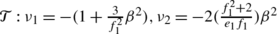
In order to study perturbations of the system (35), we consider the universal unfolding of the linear vector field B z used in van Gils et al. [5].

The above unfolding of B(λ) may also be found from the viewpoint of versal deformations of matrices, as in Arnold [9], allowing for rescaling of time.

Now, making the observation that z ₁=0 implies z ₂=0, we choose new coordinates (r,θ) satisfying r>0 and

$$z_1=r{\mathrm{e}}^{{\mathrm{i}}\theta}, \qquad z_2=r{ \mathrm{e}}^{{\mathrm{i}}\theta }w, \quad w=u+{\mathrm{i}}v. $$

It is obvious that ϕ _j (j=1,2) are even functions in r, then the normal form is odd in r. Therefore, we could make a further reduction, defining

$$\rho=r^2,\quad\rho>0, $$

thus we could obtain a set of three real equations, independent of the phase variable θ

$$ \everymath{\displaystyle} \begin{array}{@{}rcl} \dot{\rho} &=& 2\rho(\alpha+u+c_1\rho)+\mathrm{h.o.t.},\\[1mm] \dot{u} &=& \mu_1-u^2+v^2+\rho(e_1+2f_2v)+\mathrm{h.o.t.},\\[1mm] \dot{v}&=& \mu_2-2uv+\rho(f_1-2e_2v)+\mathrm{h.o.t.}, \end{array} $$

(36)

and

$$\dot{\theta}=1+v+d_1\rho+\mathrm{h.o.t.}, $$

where

$$c_1=\operatorname{Re}\biggl(\frac{a_1}{\tau^*\omega^*}\biggr), $$

$$e_1=\operatorname{Re} {\frac {b_1}{\tau^{*2}\omega^{*2}}}, \quad e_2=\operatorname{Re} \biggl(\frac{b_2}{\tau^*\omega^*}\biggr); $$

$$d_1=\operatorname{Im}\biggl(\frac{a_1}{\tau^*\omega^*}\biggr), $$

$$f_1=\operatorname{Im} {\frac {b_1}{\tau^{*2}\omega^{*2}}}, \quad f_2=\operatorname{Im} \biggl(\frac{b_2}{\tau^*\omega^*}\biggr). $$

In order to blow up the dominant terms in the above equations, we define the rescaled variables by

$$ \everymath{\displaystyle} \begin{array}{@{}l} \rho=\varepsilon^2\hat{\rho}, \qquad u=\varepsilon\hat{u}, \qquad v=\varepsilon\hat{v}, \qquad \varepsilon t=\hat{t}, \\ [1mm] \alpha=\varepsilon\beta, \qquad \mu_1=\varepsilon^2\nu_1, \qquad \mu_2=\varepsilon^2\nu_2. \end{array} $$

(37)

Substituting (37) into (36) and dropping the hats, we have

$$ \begin{array} {@{}rcl} \dot{\rho} &=& 2\rho( \beta+u)+\varepsilon2c_1\rho^2+O\bigl( \varepsilon^2\bigr), \\[2mm] \dot{u} &=& \nu_1-u^2+v^2+e_1 \rho+2\varepsilon f_2v+O\bigl(\varepsilon^2\bigr), \\[2mm] \dot{v}&=& \nu_2-2uv+f_1\rho-2\varepsilon e_2v+O\bigl(\varepsilon^2\bigr), \end{array} $$

(38)

We assume that e ₁≠0≠f ₁ in the following analysis, then we can rescale e ₁ to ±1. By using a similar argument to that in van Gils et al. [5], we have the following results.

Theorem 5

• (1) The system (36) undergoes a codimension-1 pitchfork bifurcation on the primary bifurcation variety 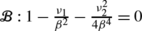, shown in Fig. 1.

  Fig. 1

  

  Multiplicities of periodic solutions for β≠0. (a) e ₁=1; (b) e ₁=−1

• (2) A codimension-1 limit point or “saddle-node bifurcation” occurs on the limit point variety which is the surface generated by the ray $N: f_{1}(e_{1}\nu_{2}-f_{1}\nu_{1})+\beta^{2}(1+f_{1}^{2})=0$ in the system (36), shown in Figs. 1 and  2, and when the phase equation is restored, we derive a saddle-node bifurcation of periodic orbits. This in turn persists as a two-dimensional variety for the original system (5).

  Fig. 2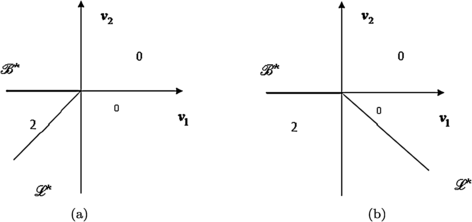

  

  Multiplicities of periodic solutions for β=0. (a) e ₁=1; (b) e ₁=−1

• (3) The symmetric cusp variety $\mathcal{E}$ at which the two surfaces and meet in the planes β ²=1 is the ℤ₂ symmetric version of the standard cusp (with vanishing cubic bifurcation coefficient), shown in Fig. 1. And that the variety $\mathcal{E}$ persists for the full system follows from the preservation of S ¹ symmetry on the periodic orbits [10].

• (4) System (36) undergoes a double Hopf bifurcation which has linear codimension-2 and occurs on the one-dimensional double Hopf bifurcation variety in the β=0 plane, shown in Fig. 2. In addition, it gives rise to mixed-mode secondary Hopf bifurcations (of 2-tori) and there is a possibility of a 3-torus arising from the interaction of these two Hopf bifurcations [11].

• (5) For ν ₁<0 and bounded away from 0, the Hopf variety is close to the lower branch of a parabola in the (ν ₁,ν ₂) plane, which lies between and , asymptotically β→0. For ν ₁>0 and bounded away from 0, only in the case e ₁=−1, 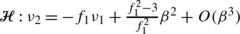lies just below the limit point variety , as β→0 in (ν ₁,ν ₂) coordinates. These Hopf bifurcations extend to system (36) provided the standard nondegeneracy conditions hold.

• (6) Assume that β≠0 and define a path in ℝ³ which we call the Bogdanov–Takens variety at which the Hopf variety and the limit point variety intersect, then the Bogdanov–Takens bifurcation occurs in the case e ₁=1. Meanwhile, the Bogdanov–Takens variety always lies to the left of the cusp variety $\mathcal{E}$ in the (ν ₁,ν ₂) plane, and persists in the full three-dimensional system (36).

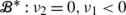
• (7) Assume that β=0, the zero and pure imaginary eigenvalues occur simultaneously along the ray N=0,β=0,ν ₁>0 of codimension-2, which we call the {1,i,−i} variety , shown in Fig. 2.

Theorem 6

For every value of the parameters α, μ ₁, μ ₂ in a neighborhood of 0, Eq. (35) has 0, 1, or 2 periodic orbits which lie inside a wedge of second-order contact about the z ₁ plane in the (z ₁,z ₂) coordinates. For each fixed small β≠0, the corresponding (ν ₁,ν ₂) plane has three open connected components, labeled by the number of periodic orbits in each component, as shown in Fig. 1. If β=0, then there are two open connected components, containing 0 or 2 periodic solutions, as shown in Fig. 2.

5 Numerical simulations

In this section, we shall present some numerical results of the system (5) with δ=0 to verify the analytical predictions obtained in the pervious section. Let us consider the following system:

$$ \begin{array}{@{}rcl} \dot{x}(t)&=&y(t), \\[2mm] \dot{y}(t)&=&-x(t)+0.01\bigl(1-x^2(t)\bigr)y(t) \\[2mm] &&{}+\gamma\bigl(x(t-2)\bigr). \end{array} $$

(39)

We solve (8) with ε=0.01 and τ=2 for ω and obtain (ω _j ,γ _j ), which are given in Table 1. It is shown that $\frac{\tau\gamma ^{2}_{1}}{1+\omega_{1}^{2}}<\varepsilon$ and $\frac{\tau\gamma ^{2}_{j}}{1+\omega_{j}^{2}}>\varepsilon$ for all j≠1, i.e., $\operatorname{Re}\lambda'_{\gamma}(\varepsilon,\tau,\gamma_{j})<0$ for all j≤1 and $\operatorname{Re}\lambda'_{\gamma}(\varepsilon,\tau,\gamma _{i})>\nobreak 0$ for all i>1. Meanwhile, we get $\bar{\omega}=\sqrt{2-\varepsilon^{2}}\approx1.4142$ and $\tau_{0}=\frac{1}{\bar{\omega}}(\pi-\arcsin\varepsilon\bar {\omega })\approx2.2115>\tau$ (see Lemma 4(iv)). By Theorem 3, the equilibrium (0,0) is asymptotically stable for γ∈(0.011,1), and unstable for all γ∈(−∞,0.011)∪(1,+∞), which is shown in Figs. 3–6.

Fig. 3

Numerical simulations of system (39) with γ=−0.5<γ ₁≈0.011. (a) The equilibrium (0,0) is unstable; (b) an asymptotically stable periodic solution is bifurcated from (0,0)

Table 1 List of parameters under ε=0.01 and τ=2

It follows from Corollary 1 that when δ=0 and τε<2, the Hopf bifurcation occurs as γ crosses γ ₁ (respectively, γ _j (j≥2)) to the left (respectively, right), and the bifurcating periodic solutions are orbitally asymptotically stable (respectively, unstable). When γ=2>γ ₂≈1.4505, the equilibrium (0,0) is unstable, and the bifurcating periodic solutions are unstable, which is shown in Figs. 4 and 6. If γ=−0.5<γ ₁≈0.011, then the equilibrium (0,0) is unstable, and the corresponding bifurcating periodic solutions are asymptotically stable, which is shown in Figs. 3 and 5.

Fig. 4

Numerical simulations of system (39) with (a) γ=−9<γ ₋₁≈−8.7574 and (b) γ=−40<γ ₋₂≈−39.997, where the equilibrium (0,0) is unstable

Fig. 5

Numerical simulations of system (39) with (a) γ=0.8∈(0.011,1) and γ=1.2>1. In (a) the equilibrium (0,0) is asymptotically stable, but in (b) the equilibrium (0,0) is unstable

Fig. 6

Numerical simulations of system (39) with γ=2>γ ₂≈1.4505, where the equilibrium (0,0) is unstable, and the periodic solution bifurcated from (0,0) is unstable

Unfortunately, the existence of periodic solutions via 1:1 resonant Hopf bifurcation can not been verified because it is difficult to seek suitable initial values such that the solution of associated initial value problem may converge to them even though the periodic solutions are stable.

6 Conclusions

In this paper, we present a detailed study of Hopf bifurcation in the van der Pol equation with delayed feedback. By analyzing the associated characteristic equation, we have shown that the Hopf bifurcation occurs at a set of parameter values $\mathcal{H}$ and obtained formulae determining the stability of the zero solution. Using the normal form theory and the center manifold theorem, the stability and the direction of the Hopf bifurcation with simple imaginary eigenvalues are determined. Specifically, we investigate a generalized Hopf bifurcation corresponding to non-semisimple double imaginary eigenvalues (case of 1:1 resonance), which has linear codimension-3, and a center subspace of dimension-4. Using a normal form approach, we find that there exist 0, 1, or 2 small-amplitude periodic solutions. Moreover, we locate one-dimensional varieties in the parameter space ℝ³ on which the system has three different types of codimension-1 singularities and four different types of codimension-2 singularities.

Obviously, there is a question that is worthy of further investigation. In this paper, we only consider a single van der Pol oscillator with delayed feedback. It is interesting to generalize our results in this paper to delay-coupled van der Pol oscillators and other modified van der Pol oscillators. For example, Liao et al. [12] investigated the linear stability and standard Hopf bifurcation for a van der Pol equation with a distributed time delay. Song [13] investigated the spatiotemporal patterns of Hopf bifurcating periodic oscillations in a pair of van der Pol oscillators with delayed velocity coupling. Algaba et al. [14, 15] considered high codimensional bifurcations in a modified van der Pol-Duffing electronic circuit. Wirkus and Rand [16] studied the dynamics of a pair of van der Pol oscillators where the coupling is chosen to be through the damping terms but not of diffusive type. However, to consider resonant Hopf bifurcation in these models, further discussion is needed.

References

Van der Pol, B.: A theory of the amplitude of free and forced triode vibrations. Radio Rev. 1, 701–710, 754–762 (1920)
Atay, F.M.: Van der Pol’s oscillator under delayed feedback. J. Sound Vib. 218(2), 333–339 (1998)
Wei, J., Jiang, W.: Stability and bifurcation analysis in van der Pol’s oscillator with delayed feedback. J. Sound Vib. 283, 801–819 (2005)
Jiang, W., Wei, J.: Bifurcation analysis in van der Pol’s oscillator with delayed feedback. J. Comput. Appl. Math. 213, 604–615 (2008)
van Gils, S.A., Krupa, M., Langford, W.F.: Hopf bifurcation with non-semisimple 1:1 resonance. Nonlinearity 3, 825–850 (1990)
Ruan, S., Wei, J.: Periodic solutions of planner systems with two delays. Proc. R. Soc. Edinb. 129A, 1017–1032 (1999)
Dieudonné, J.: Foundations of Modern Analysis. Academic Press, New York (1996)
Namachchivaya, N.S., Doyle, M.M., Langford, W.F., Evans, N.W.: Normal form for generalized Hopf bifurcation with non-semisimple 1:1 resonance. Z. Angew. Math. Phys. 45, 312–324 (1994)
Arnold, V.I.: On matrices depending on parameters. Russ. Math. Surv. 26, 29–43 (1971)
Golubitsky, M., Langford, W.F.: Classification and unfoldings of degenerate Hopf bifurcations. J. Differ. Equ. 41, 375–415 (1981)
Iooss, G., Langford, W.F.: Conjectures on the routes to turbulence via bifurcations. Nonlinear Dyn. 357, 489–505 (1980)
Liao, X., Wong, K., Wu, Z.: Hopf bifurcation and stability of periodic solutions for van der Pol equation with distributed delay. Nonlinear Dyn. 26, 23–44 (2001)
Song, Y.: Hopf bifurcation and spatio-temporal patterns in delay-coupled van der Pol oscillators. Nonlinear Dyn. 63, 223–237 (2011)
Algaba, A., Freire, E., Gamero, E., Rodriguez-Luis, A.J.: A tame degenerate Hopf–Pitchfork bifurcation in a modified van der Pol–Duffing oscillator. Nonlinear Dyn. 22, 249–269 (2000)
Algaba, A., Freire, E., Gamero, E., Rodriguez-Luis, A.J.: Analysis of Hopf and Takens–Bogdanov bifurcations in a modified van der Pol–Duffing oscillator. Nonlinear Dyn. 16, 369–404 (1998)
Wirkus, S., Rand, R.H.: The dynamics of two coupled van der Pol oscillators with delay coupling. Nonlinear Dyn. 30, 205–221 (2002)
Acknowledgements
This work supported in part by the NSFC (Grant No. 11271115), by the Doctoral Fund of Ministry of Education of China, and by the Hunan Provincial Natural Science Foundation (Grant No. 10JJ1001).
Author information
Authors and Affiliations
Corresponding author
Rights and permissions
About this article
Cite this article
Zhang, L., Guo, S. Hopf bifurcation in delayed van der Pol oscillators. Nonlinear Dyn 71, 555–568 (2013). https://doi.org/10.1007/s11071-012-0681-y
Received:
Accepted:
Published:
Issue Date:
DOI: https://doi.org/10.1007/s11071-012-0681-y