High-capacity reversible data hiding based on multi-histogram modification

Abstract

Reversible data hiding is a technique that embeds a message into a host image with acceptable visual distortion and then recovers the image without any data loss while extracting the embedded message. The previous schemes mainly suffer from an unresolved problem that the imperceptibility of a marked image decreases severely as the embedding capacity increases. Extending the histogram modification technique, this study proposes a novel scheme that utilizes multiple histograms to increase embedding capacity while keeping marked-image quality. Unlike most histogram modification schemes, the multi-histogram scheme does not suffer from overflow and underflow during histogram shift. This scheme can yield the embedding capacity of 1 bit per pixel (bpp) at the PSNR of 48.13 db for a 512 × 512 grayscale image. To reduce the overhead during message embedding, the work further proposes an iterative multi-histogram scheme. Comprehensive experimental results show that both the schemes can achieve high embedding capacity and image quality.

1 Introduction

Data hiding [25, 26] is a technique to embed a message into a host image with acceptable visual distortion and to extract the message from the marked host image. In most applications of data hiding, such as copy control and content authentication, some permanent distortion may have happened to the host image after the message extraction. However, some data-hiding applications, especially in medical, military, and legal domains, are required to extract the message without any distortion of the host image. This requirement leads to an interesting hiding technique – reversible, lossless, distortion-free, or invertible data hiding, in which a host image must be recovered completely as an embedded message has been extracted out.

Many reversible schemes were proposed to enhance data-hiding capacity and image-embedding quality. Fridrich et al. [5] devised a least significant bit (LSB)-based reversible algorithm that could hide a message into the quantized DCT coefficients. Celik et al. [2] proposed a generalized-LSB (G-LSB) scheme compressing the quantization residuals of pixels to improve hiding payloads. The study in [6] presented a lossless data-hiding technique with high capacity by embedding data bits into the state of each group of pixels. Tian [18] designed a high-capacity reversible scheme based on the difference expansion transform of a pair of pixels. Extending Tian’s method, Alattar’s work [1] embedded data using the difference expansion transform of vectors, and reduced the difference values using a generalized integer transform of vectors. Thodi et al. [17] devised an effective method for data embedding by combining prediction-error expansion and histogram shifting. Wang et al. [23] presented two difference-expansion data-hiding schemes for 2-D vector maps. Based on the integer Haar wavelet transform, Hu et al. [9] proposed a new difference-expansion embedding algorithm, which utilized the horizontal as well as vertical difference images for data hiding. The study in [10] increased embedding capacity by improving the compressibility of the overflow location map. Weng et al. [24] utilized the invariability of the sum of pixel pairs and the pairwise difference adjustment (PDA) to achieve large hiding capacity with small distortion. Lin et al. devised a lossless scheme based on three-pixel block differences [12]. Chang et al. proposed an embedding scheme based on the side match vector quantization (SMVQ) [3]. The scheme in [22] embedded the secret bits into the VQ index table by modifying the index value according to the difference of neighboring indices. Lee et al. [11] divided an image into blocks and embedded watermark data into the high-frequency wavelet coefficients of each block.

Ni et al. [14] proposed a simple reversible algorithm based on histogram modification that used peak-zero points to embed data into an image. Fallahpour et al. [4] divided an image into multiple blocks, and found a peak-zero point for each block to embed data. Lin et al. [13] presented a multilevel histogram-modification hiding strategy to yield high embedding capacity as well as low distortion. This strategy embedded data bits into the pixels associated with the peak points in the difference image histogram. Tsai’s study [19] presented a histogram-modification algorithm that worked on VQ indices. Tsai et al. [20] examined the similarity of neighboring pixels in an image, and embedded data into the residual histogram of the predicted errors of the host image. Tai et al. [16] devised an embedding scheme based on the histogram modification and the pixel difference, and used a binary tree structure to save the pairs of peak-zero points.

The above schemes all suffer from an unresolved problem that the imperceptibility of a marked image decreases severely when the embedding capacity increases. Extending the histogram modification technique, this study proposes a multi-histogram modification scheme, which utilizes multiple histograms to increase hiding capacity while keeping high image quality. Unlike most exiting histogram modification schemes, the multi-histogram scheme does not suffer from overflow and underflow during histogram shift. This scheme can yield the embedding capacity of 1 bit per pixel (bpp) at the PSNR of 48.13 db for a 512 × 512 grayscale image. However, the scheme may require numerous peak-zero pairs. To reduce the required pairs, the work further proposes an iterative multi-histogram scheme. Comprehensive experimental results show that both the schemes can achieve high embedding capacity and image quality.

The rest of this paper is organized as follows. Next section presents the proposed reversible data-hiding scheme. Section 3 includes the experimental results and performance comparisons. Conclusions are drawn in Section 4.

2 The multi-histogram scheme

The histogram-based schemes generally share similar steps to embed data into a host image. The schemes first adopt different approaches, such as pixel grayscale [14] or difference [13, 20], to generate a histogram. The histogram is then scanned to obtain the pairs of peak and zero points, in which each pair can be utilized to hide data by shifting histogram. Clearly, the larger the difference between the peak and zero points is, the higher the data-hiding capacity is. Thus, the previous researches mainly investigate how to generate a histogram that has the peak-zero pairs with large differences. In a different manner, this work proposes an approach that generates multiple histograms for a host image, in which each histogram has several peak-zero pairs to hide data. Figure 1 shows that the proposed scheme includes three stages – multiple-histogram generation, data embedding, and extraction. The first stage generates several histograms for a host image H. By using the histograms, the data embedding process encodes the message M into the image H, and yields a secret key. With the secret key and the marked image H’, the final stage restores the image H and the message M. We next present the details of the proposed data-hiding algorithm.

Fig. 1

The concept of the proposed scheme

2.1 Multiple-histogram generation

This paper first defines a pixel set $A = \left\{ {0,{1},{2}, \ldots, {255}} \right\}$, where each element represents a possible value of a pixel in an 8-bit grayscale image. An m-pixel grayscale image H is scanned in a sequential order, say, row-by-row, or column-by-column, from left to right to generate a pixel sequence $S = {x_{{1}}}\bullet {x_{{2}}}\bullet \cdots \bullet {x_i}\bullet \cdots \bullet {x_m}_{{ - {1}}}\bullet {x_m}$,¹ where x _i ∊ A, ${1} \leqslant i \leqslant m$. Let $s = {a_{{1}}}\bullet {a_{{2}}} \ldots {a_n}_{{ - {1}}}\bullet {a_n}$ be an n-pixel subsequence of the sequence S, where s ⊂ S. For instance, given $S = {1}\,\bullet \, {2}\,\bullet \,{3}\,\bullet \,{5}\,\bullet \,{9}$ and n = 2, the subsequence s could be 1•2, 5•9, and so on. Generally, let P be a set containing all the possible patterns (or combinations) of an n-pixel subsequence. Because the set A contains 256 elements, the maximum number of the elements in P equals 256ⁿ. For example, for n = 2, there exist 256² possible patterns for a 2-pixel subsequence. The basic concept behind our scheme is to generate a histogram for each pattern. The steps to generate histograms for n-pixel patterns are as the following.

• 1. Define a dummy pixel sequence $V = {v_{{1}}}\bullet {v_{{2}}}\bullet \cdots \bullet {v_i}\bullet \cdots \bullet {v_n}_{{ - {1}}}\bullet {v_n}$, where v _i ∊ A, ${1} \leqslant i \leqslant n$. Here, the pixels of the sequence V can be chosen arbitrarily. We then join the sequence V into the front of the sequence S, and obtain a new sequence V • S.

• 2. Create a histogram table, as illustrated in Table 1. Each cell indicates the times that a pixel q (q ∊ A) follows a pattern p (p ∊ P) when the sequence V • S is scanned. The value of a cell is denoted by r(q|p). At the start, all the values are initialized to zero. This paper later shows that each row can generate a histogram for hiding data.

  Table 1 The histogram table for n-pixel patterns

• 3. Scan the sequence V • S one pixel by one pixel to find each pattern p and its following pixel q, and to increase the corresponding count r(q|p) in Table 1 by one. We use a virtual sliding window W to implement the scanning, as illustrated in Fig. 2. Figure 2-(a) shows that the window W constantly contains n + 1 pixels in order, where the first n pixels constitute a found pattern p, and the following pixel q is the n + 1th pixel. Initially, the window is put in the beginning of the sequence V • S, and thus the first found pattern p is exactly the sequence V and the following pixel q is the pixel x ₁, as shown in Fig. 2-(b). The count r(x ₁|V) increases by one. We then slide the window W forward by one pixel, as illustrated in Fig. 2-(c). The pattern p and the following pixel q become ${v_{{2}}}\bullet {v_{{3}}}\bullet \cdots \bullet {v_n}_{{ - {1}}}\bullet {v_n}\bullet {x_{{1}}}$ and x ₂, respectively. The count $r({x_2}\left| {{v_2}} \right.\bullet {v_{{3}}}\bullet \cdots \bullet {v_n}_{{ - {1}}}\bullet {v_n}\bullet {x_{{1}}})$ increases by one. Repeat the process until the last pattern $p = {x_m}_{{ - n}}\bullet {x_m}_{{ - n + {1}}}\bullet \cdots \bullet {x_m}_{{ - {2}}}\bullet {x_m}_{{ - {1}}}$ and the pixel q = x _m are found, and the corresponding count $r({x_m}\left| {{x_m}_{{ - n}}} \right.\bullet {x_m}_{{ - n + {1}}}\bullet \cdots \bullet {x_m}_{{ - {2}}}\bullet {x_m}_{{ - {1}}})$ is updated. We can totally obtain m patterns, and Table 1 records the distribution of pixels on each pattern. With this table, the proposed approach further generates a histogram for each pattern in which the horizontal values are the pixels in the set A, and the vertical values are the times that the pixels are found immediately after the pattern.

  Fig. 2

  

  Multiple-histogram generation

An example is next used to illustrate the multiple-histogram generation, and this example is also used to explain the data embedding and extracting processes later. Suppose $S = 0\,\bullet {1}\,\bullet {2}\,\bullet 0\,\bullet {2 }\bullet {1}\,\bullet 0\,\bullet {1}\,\bullet {2}$, and n = 1. There exist 256 patterns in set P, such as 0, 1, 2, 3, and so on. Here, we simply assume V = 0, and $V\,\bullet S = 0\,\bullet 0\,\bullet {1}\,\bullet {2}\,\bullet 0\,\bullet {2}\,\bullet {1}\,\bullet 0\,\bullet {1}\,\bullet {2}$. Figure 3 illustrates the entire histogram generation. Step 0 initially sets all the cells in the histogram table to zero. We then scan the sequence V • S from the beginning via the window W. The first step finds p = 0 and q = 0, and updates the corresponding cell colored gray in the histogram table. By moving the window W along the sequence V • S by one pixel, each step can find a new pattern p and its following pixel q. Step 9 finally obtains p = 1 and q = 2, and completes the entire histogram table, which includes the distribution of each pixel on each pattern. For instance, the first row of the histogram table indicates that for the pattern p = 0, the pixel “0” was found once, the pixel “1” twice, the pixel “2” once, and other pixels zero times. Due to n = 1, the generated table has 256 rows, and each row can be considered as a histogram for a pattern. The next subsection will explain how to apply the histogram table to hide data.

Fig. 3

Illustration of multiple-histogram generation

2.2 Data embedding algorithm

Assume that $M = {m_{{1}}}\bullet {m_{{2}}}\bullet \cdots \bullet {m_i}\bullet \cdots \bullet {m_k}_{{ - {1}}}\bullet {m_k}$ is a k-bit to-be-embedded sequence, where m _i ∊ {0, 1}, ${1} \leqslant i \leqslant k$. The following process embeds the sequence M into the sequence S, and obtains a marked sequence S’.

• 1. Scan the generated histogram table row by row to find peak-zero pairs of each pattern p based on the count values r(q|p). Figure 4 illustrates the peak-zero pairs of a pattern p. The height of a rectangle represents the count values r(q|p) at a pixel q. In the figure, the peak points A, B, and C are the local maximum count values in the histogram of the pattern p, while each peak must correspond to a zero point (i.e., A’, B’ and C’) whose count value is zero. The steps to find peak-zero pairs for a pattern are as below.

  • Scan the row corresponding the pattern on the Table 1 from left to right. Once finding a non-zero count value, set a peak to this pixel.

  • Scan the row continuously. If a larger or equal count value of a pixel is found, update the peak to the new pixel.

  • Repeat the above step until finding a count value of a pixel zero, and set a zero point to the pixel. A peak-zero pair is thus found.

  • Repeat the above three steps until finishing scanning the row. Any peak point without corresponding a zero point is abandoned.

  Fig. 4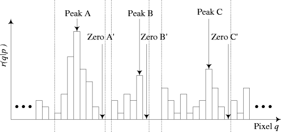

  

  Illustration of the peak-zero pairs

  The found peak-zero pairs are utilized to embed and extract data. The pairs and the dummy sequence V constitute the secret key mentioned in Fig. 1. The current histogram-based schemes generate secret keys based on the characteristics of a host image. The secret keys can be detective once the host image is revealed [15]. To avoid this problem, the proposed scheme additionally requires the dummy sequence V to restore a marked image. The length and the contents of the sequence are given randomly, and are hard to detect. The scheme thus exhibits higher security. Furthermore, the multi-histogram scheme, unlike most histogram-based schemes, does not suffer from the problem of overflow. From the steps to determine peak-zero pairs, we can find that the maximum pixel 255 does not become a peak point because the corresponding zero point does not exist. Thus, the overflow caused by adding one to the pixel value 255 does not happen. In addition, most previous schemes, such as [4, 13, 14, 16, 19, 20], may generate no peak-zero pair for particular man-made images, and cannot hide data into the images. In contrast, the proposed scheme can adjust the value and the length of the dummy sequence V to yield peak-zero pairs for multiple histograms, and thus gains the minimum capacity larger than zero.

• 2. Scan the sequence V • S by moving the sliding window W one pixel by one pixel. For each found pattern p and the following pixel q, we compare the pixel q with the peak-zero pairs of the pattern p.

  • If the pixel q is not located between a peak point and an associated zero point, add the pixel q into the end of the marked sequence S’.

  • If the pixel q is a peak point, and add the pixel q + m _i into the end of the sequence S’. In this case, the scheme embeds a bit m _i of the sequence M into the sequence S.

  • If the pixel q is not a peak point but a point between a peak point and an associated zero point, add the pixel q + 1 into the end of the sequence S’.

This paper next demonstrates the embedding process by using the previous example in Fig. 3. Assume $M = {1}\,\bullet 0\,\bullet {1}\,\bullet 0\,\bullet {1}\,\bullet 0$. We first scan each row of the table generated by step 9 in Fig. 3 to find peak-zero pairs for each pattern. The results are listed in Table 2, where the found peak count values are bold, and the zero values are colored gray. For example, there exists one peak-zero pair, (1,3), for pattern “0” in the first row. The second row contains two pairs, (0,1) and (2,3) for pattern “1”.

Table 2 The histogram table for the example in Fig. 3

Our scheme then scans the sequence V • S to hide the sequence M. Figure 5 demonstrates the entire process. When Step 1 starts scanning the sequence V • S, the step finds p = 0 and q = 0. According to the first row of Table 2, the pixel q is not located in the peak-zero pair (1,3). Thus, the value of the pixel q is not modified, and directly becomes the first pixel of the sequence S’, colored gray. Step 2 continuously scans the sequence V • S, and finds p = 0 and q = 1. Since the pixel q is a peak point for the pattern p on Table 2, the scheme adds the pixel $q + {m_{{1}}}{ = 1 + 1 = } {2}$ into the end of the sequence S’. The third pattern found in the sequence V • S is “1”, and the following pixel q = 2 is also a peak point. The pixel $q + {m_{{2}}}{ = 2 + }0 = {2}$ thus becomes the third pixel of the sequence S’. The fourth pattern is “2”, and the following pixel “0” is outside the peak-zero pair (1,2) on the third row of Table 2. This pixel is thus directly added into the end of the sequence S’. Step 5 shows that the found pattern is “0”, and its following pixel q = 2 is not a peak but a point located between the peak-zero pair (1,3). We thus insert the pixel $q + {1 = 3}$ into the end of the sequence S’. The remaining embedding steps are similar, and please refer to Fig. 5 for the details.

Fig. 5

Illustration of data embedding

2.3 Data extracting algorithm

To extract the sequences S and M from the marked sequence S’, our scheme finds each pattern p from the sequence V • S, and finds the following pixel q from the sequence S’ by simultaneously scanning both the sequences. Here, two sliding windows are utilized to obtain patterns from the sequence V • S, and to obtain following pixels from the sequence S’. The peak-zero pairs yielded by the embedding algorithm are also used to complete the extraction process. The extraction steps are as the following.

Initially, the sequences S and M are empty, and thus V • S = V. When the sequence V • S is scanned, the pattern p found first is V. The following pixel q comes from the first element of the sequence S’, rather than the sequence S. We then compare the pixel q with the peak-zero pairs of the pattern p.

• If the pixel q is not located between a peak point and an associated zero point, add the pixel q into the end of the sequence S.

• If the pixel q is a peak point, add the pixel q into the end of the sequence S, and a bit “0” into the end of the sequence M, respectively. This means that the pixel q hides a bit “0” of the sequence M.

• If the pixel q is immediately after a peak point, add the pixel q − 1 into the end of the sequence S, and a bit “1” into the end of the sequence M. This means that the pixel q hides a bit “1” of the sequence M.

• If the pixel q is inside the value range of a peak-zero pair but neither a peak nor a point immediately following the peak, add the pixel q − 1 into the end of the sequence S.

The sliding windows are then moved forward by one pixel to find the next pattern and the following pixel. We repeat the above process until the last element of the sequence S’ is scanned, and the sequences S and M are restored completely. Note that the extraction process does not meet the problem of underflow caused by subtracting one from the pixel value zero. This is because the embedding process does not set a zero point to the pixel zero.

Figure 6 demonstrates the entire process of extracting the sequences S and M from the sequence S’ in Fig. 5. Step 1 scans the sequences V • S and S’, and obtains p = 0 and q = 0. According to the first row of Table 2, the pixel q is not located in the peak-zero pair (1,3). Thus, the pixel q is not modified, and directly becomes the first element of the sequence S, colored gray in Fig. 6. Step 2 continuously finds the next pattern p = 0 from the sequence V • S, and the following pixel q = 2 from the sequence S’. Since the pixel q immediately follows a peak point, we add the pixel q − 1 to the sequence S according to the above extracting rules, and a bit “1” becomes the first element of the sequence M. Figure 6 shows that the third pattern p is “1” and the following pixel q is “2”. Because the pixel q is a peak point, the pixel directly becomes the third element of the sequence S without changing its value, and the second bit of the sequence M is “0”. In Step 4, p = 2, and q = 0. The pixel q is directly appended into the sequence S since the pixel is outside the range of the peak-zero pair (1,2) on the third row of Table 2. The fifth pattern is “0”, and the following pixel q = 3 is inside the range of the peak-zero pair (1,3) but neither a peak nor a point immediately after the peak. We thus insert the pixel q − 1 into the end of the sequence S. Step 6 continuously finds the pattern p = 2 from the sequence V • S, and the following pixel q = 2 from the sequence S’. Since the pixel q immediately follows a peak point, we append the pixel q − 1 to the sequence S, and a bit “1” to the sequence M. The seventh pattern is “1”, and the following pixel q = 0 is a peak point. The pixel q directly becomes the new element of the sequence S, and the new bit of the sequence M is “0”. Step 8 finds the pattern p = 0 from the sequence V • S, and the following pixel q = 2 from the sequence S’. The pixel q immediately follows a peak point, and we thus append the pixel q − 1 to the sequence S, and a bit “1” to the sequence M. The last pattern is “1”, and the following pixel q = 2 is a peak point. The pixel q thus becomes the last element of the sequence S, and the last bit of the sequence M is “0”. Accordingly, the sequences S and M are restored completely.

Fig. 6

Illustration of data extraction

2.4 Pseudocode of algorithms

This subsection presents C-like pseudocode for the data embedding and extracting algorithms, and discusses the applicable implementation. Table 3 lists the definitions of the variables in the pseudocode. Figure 7 depicts the pseudocode for generating multiple histograms and embedding data. The pseudocode mainly consists of three parts. The first part uses two-tier AVL trees [7] to implement the histogram table (i.e., Table 1). The first level only contains an AVL tree, which includes all found patterns in the sequence V • S. Each found pattern has an AVL tree in the second level to save its count values (i.e., r(q|p)). For the two-tier AVL trees, each node consists of a key and a value. We use a pattern p as a key to search the first-tier AVL tree for the pointer to its second-tier AVL tree. A following pixel q is then taken as a key to search the second-tier AVL tree for the counts.

Table 3 Variable definitions in the pseudocode

Fig. 7

Pseudocode of multiple-histogram generation and data hiding

The second part of the pseudocode then determines peak-zero pairs for each found pattern. Another two-tier AVL trees are created to save peak-zero pairs. The first-tier AVL tree includes all found patterns in the sequence V • S. Each found pattern has a second-tier AVL tree to save its peak-zero pairs. We use a pattern p as a key to search the first-tier AVL tree for the pointer to its second-tier AVL tree, in which the key of each node is a peak point, and the node value is the associated zero point. The last part of the pseudocode demonstrates how to embed the sequence M into the sequence S and to generate the sequence S’. We design a function point_type() with two parameters – a pattern p and its following pixel q. The function traverses the two-tier AVL trees of peak-zero pairs, and checks whether the pixel q is a peak, a point in a peak-zero pair but not a peak, or a point not in any peak-zero pair. According to the return result, the pseudocode generates a corresponding pixel for the sequence S’.

To extract data, the pseudocode in Fig. 8 initially loads the secret key (i.e., the peak-zero pairs generated in Fig. 7) into the two-tier AVL trees as mentioned above. The first-tier AVL tree includes the found patterns in the sequence V • S. Each found pattern has a second-tier AVL tree to save its peak-zero pairs. We also design a function point_type() to traverse the two-tier AVL trees, and to determine whether a pixel q is a peak, a point following a peak, a point in a peak-zero pair but neither a peak nor a point immediately after a peak, or a point not in any peak-zero pair. According to the return result, the pseudocode restores the sequences S and M.

Fig. 8

Pseudocode of data extraction

2.5 Complexity analysis

The proposed algorithm does not apply any transform such as discrete cosine transform (DCT), discrete wavelet transform (DWT), and so on. The required processing mainly lies on generating multiple histograms for a host image, determining peak-zero pairs for each pattern, hiding messages, and doing the inverse transformation in the spatial domain. Accordingly, the execution time of the algorithm is small. To generate multiple histograms, we need to scan the image sequence S once, and to create the two-tier AVL trees. The complexity for scanning the sequence S depends on the sequence length m, and is O(m). Before deriving the entire complexity for creating the two-tier AVL trees, we first analyze the complexity of an access to the trees. Since the length of the sequence S equals m, the maximum number of the found patterns is m, and so is the maximum number of the nodes in the first-tier AVL tree. According to the study in [7], the complexity of an access to the first-tier tree is O(log m). A second-tier AVL tree stores the following pixels of a found pattern and the corresponding count values. The maximum number of the nodes in the second-tier AVL tree thus equals the number of the following pixels. The maximum number of the pixels is the element number of the set A, a constant value 256. The complexity of an access to the second-tier AVL tree is thus O(log 256). Accordingly, the complexity of an access to the two-tier AVL trees is O(log 256 log m). Because the pseudocode only uses a for-loop of m iterations to access the two-tier trees, the entire complexity for generating multiple histograms is O(m log 256 log m).

The pseudocode to determine peak-zero pairs for each found pattern contains a nested for-loop to access another two-tier AVL trees, where the outer and the inner loops have m and 256 iterations, respectively. Thus, the complexity of this step is O(256 m log 256 log m), too. Similarly, the pseudocode to embed the message sequence M to the sequence S also includes a for-loop of m iterations to access the two-tier trees, and its complexity is thus O(m log 256 log m). According to the previous analysis, the complexity of the data-hiding algorithm is O(256 m log 256 log m). Finally, the data-extraction pseudocode contains a for-loop of m iterations to access the two-tier trees; therefore, the complexity is the same as that of the data-hiding algorithm, O(m log 256 log m).

2.6 Lower bound of the PSNR for a marked image

The lower bound of the peak signal-to-noise ratio (PSNR) of a marked image generated by the proposed algorithm versus the original image can be proved larger than 48 dB as follows. It is clearly observed from the embedding algorithm that the pixels whose values are between a peak point and a zero point are either added by one or unchanged. Therefore, in the worst case, the values of all the pixels are increased by one, implying that the resultant mean square error (MSE) at most equals one, i.e., MSE = 1. This leads to the PSNR of the marked image versus the original image being

$$ PSNR = 10 \times {\log_{{10}}}\left( {\frac{{255 \times 255}}{{MSE}}} \right) \approx 48.13 $$

(1)

In short, the lower bound of the PSNR of a marked image generated by the proposed algorithm is 48.13 dB, which is also supported by the following experiments.

3 Experimental results and comparison

This work conducted several experiments to evaluate the performance of the proposed scheme on hiding capacity and quality of a watermarked image. The test data were commonly used grayscale images sized 512 × 512 [21], including Lena, Baboon, Barbara, Peppers, and F-16, as shown in Fig. 9. We used the Perl language to implement the data hiding and extraction algorithms. The test bed was a personal computer, equipped with an Intel Q8400 CPU and 4 GB DRAM. The execution time of the embedding algorithm varied from 3 to 40 s, and depended on the value of the number n. The bigger the value was, the longer the execution time was. With the increasing of the value, the program would consume much time to determine peak-zero pairs, and thus the entire execution time became long. In comparison with the embedding algorithm, the extraction algorithm yielded relatively smaller execution time, ranging from 2 to 6 s, because the extraction process did not require generating the peak-zero pairs.

Fig. 9

Five test images: (a) Lena; (b) Baboon; (c) Barbara; (d) Pepper; (e) F-16

3.1 Performance comparison at different pattern length n

Table 4 lists the hiding capacity and the PSNR at various pattern length n, where the size of the secret key is not taken into account. It is clear that the payload increases with larger pattern length n. For Lena, Baboon, Barbara, and Peppers, their payloads almost equal the image pixel size (i.e., 512 × 512) when n ≥ 4. We also note that the average PSNR for all the test images is above the theoretical lower bound 48.13 db. Figure 10 shows the hiding capacity in terms of bpp. For all the test images, their payload size is larger than 0.9 bpp when n ≥ 6. For Lena, Barbara, and Peppers, their payloads even equal 1 bpp when n ≥ 9. The PSNR of the watermarked images is plotted against the pattern length n for the test images in Fig. 11. The PSNR is always larger than 48.13 db at different pattern length n. Figure 12 further depicts the relationship between hiding capacity and image quality in terms of bpp and PSNR. With the increasing of the capacity, all the PSNRs are close to the lower bound of 48.13 db.

Table 4 Hiding capacities for test images at different pattern length n

Fig. 10

Hiding capacities in bpp at different pattern length n

Fig. 11

PSNR for the test images at different pattern length n

Fig. 12

Hiding capacity versus image quality for different test images

This work next investigates the size of the secret key during embedding an image. As mentioned previously, the secret key is composed of the dummy sequence and the peak-zero pairs. The dummy sequence is far smaller than the whole peak-zero pairs, and we thus only consider the required peak-zero pairs. Figure 13 shows the hiding capacity contributed by each peak-zero pair for the image Lena at various pattern length n. For n = 1, the number of the peak-zero pair is 3359. The first pair can contribute 308 embedding bits (i.e., peak value). With the increasing of the pair number,² the contribution declines significantly. There are 2102 (i.e., two-of-third) pairs hiding only one data bit. Additionally, with the growing of the pattern length n, the embedding bits contributed by the beginning peak-zero pairs go down quickly. For example, the first pairs respectively contribute 54, 19, 10, 6, 5, 5, 5, 5, and 5 embedding bits for n = 2 to 10. The figure further indicates that the larger the pattern length n is, the less efficient the data embedding by a peak-zero pair is. The result is also supported by Fig. 14, which depicts the accumulated embedding capacity versus the peak-zero number at different pattern length n. Given the fixed number of peak-zero pairs, the scheme at n = 1 yields far larger hiding capacity than the scheme at other cases. This figure also shows that the scheme can increase the embedding capacity by enlarging the value of n at the cost of numerous peak-zero pairs. For instance, for n = 9, the scheme yields the capacity of 1 bpp; however, the pair number, 259616, nearly equals the pixel size of the image Lena, 262144.

Fig. 13

The hiding capacity contributed by each peak-zero pair for the image Lena

Fig. 14

The accumulated hiding capacity contributed by peak-zero pairs for the image Lena

To reduce the number of peak-zero pairs, this work proposes the iterative multi-histogram scheme. The concept is as the following. For n = 1, the beginning peak-zero pairs perform embedding efficiently, as indicated in Figs. 13 and 14. Thus, we can only choose the beginning pairs to hide data during an embedding process, and repeat the embedding process several times to increase capacity. Let pair_no and iterative_no be the number of the selected pairs and the repeating times, respectively. Table 5 lists the hiding capacity and the PSNR for the iterative scheme, where n = 1, pair_no = 250, and iterative_no = 1. The overhead comes from a 256 × 256 bitmap, which saves the location of peak-zero pairs and is compressed by bzip2 [8]. Figures 15 and 16 further show the pure payload and the marked-image quality for the test images at various iterative times. With the increasing of the iterative times, the pure payload grows but the PSNR declines. For example, for the image Lena, the capacity and the PSNR are 0.16 bpp and 45.05 db at iterative_no = 2, and become 0.83 bpp and 31.59 db at iterative_no = 10. Figure 17 shows the visual impacts of the watermarked images at various iterative times for Lena and Barbara, where n = 1 and pair_no = 250. For iterative_no = 10, the visual distortion is still small and the PSNR is higher than 31 dB. In general, the watermarked images are hardly distinguished from the original images.

Table 5 Hiding capacity and distortion for the iterative multi-histogram scheme

Fig. 15

The pure payload of the iterative scheme for the test images

Fig. 16

The image quality of the iterative scheme for the test images

Fig. 17

Watermarked images Lena and Barbara. (a) 50.89 db embedded with 0.07 bpp at iterative_no = 1; (b) 31.59 db embedded with 0.83 bpp at iterative_no = 10; (c) 51.14 db embedded with 0.05 bpp at iterative_no = 1; (d) 31.91 db embedded with 0.61 bpp at iterative_no = 10

3.2 Performance comparison with other recent schemes

Recently, many reversible data-hiding schemes have been proposed to increase hiding capacity at low image distortion. Figure 18 compares the hiding capacity of the Lena image in bpp versus the image quality in PSNR yielded by the proposed schemes and other existing reversible schemes [1, 2, 4, 13, 14, 16, 18, 19]. Note that the proposed schemes and the studies in [4, 13, 14, 16, 19] are based on histogram modification, whereas the schemes [1, 18] are performed on the foundation of difference expansion. The particular parameter settings of these schemes are as the following. The proposed iterative scheme selects the first 250 peak-zero pairs during each embedding process at n = 1. Alattar’s scheme [1] is spatial and triplet-based. The algorithm of Ni et al. [14] only uses two peak-zero pairs, while Tsai’s scheme [19] utilizes three. Fallahpour et al. [4], Lin et al. [13], and the proposed scheme do not include the overhead information of histogram modification in the image itself with the payload, while other schemes (including the proposed iterative scheme) take the overhead into account for the hiding capacity. The evaluation results show that the proposed scheme achieves relatively higher embedding capacity and image quality than the existing schemes under the condition without including the overhead information of histogram modification. The proposed scheme can even yield the hiding capacity of 1 bpp at the PSNR of 48.13 db. When the overhead is further taken into account for the capacity, the pure payload yielded by the proposed iterative scheme is still close to those by Tai et al. [16] and Tian [18]. Accordingly, the proposed schemes achieve high capacity with low distortion under various conditions.

Fig. 18

Performance comparison with existing schemes on image Lena

4 Conclusions

This paper presents an efficient extension of the histogram modification technique by considering multiple histograms rather than a single one. The previous histogram modification schemes mainly generate a histogram to collect pairs of peak and zero points. The approach of a single histogram may limit the number of peak-zero pairs, and thus restricts the maximum hiding capacity. To alleviate this limitation, we propose the multi-histogram scheme, which can obtain more peak-zero pairs to achieve higher embedding capacity at lower image distortion. To reduce the overhead during data embedding, the work further proposes the iterative multi-histogram scheme. Comprehensive experimental results show that both the schemes well improve the embedding capacity and the image quality. Therefore, they are very appropriate for data-hiding applications that require high capacity and low distortion.

References

Alattar AM (2004) Reversible watermark using the difference expansion of a generalized integer transform. IEEE Trans Image Process 13(8):1147–1156
Celik MU, Sharma G, Tekalp AM, Saber E (2005) Lossless generalized-LSB data embedding. IEEE Trans Image Process 4(2):253–266
Chang C-C, Tai W-L, Lin C-C (2006) A reversible data hiding scheme based on side match vector quantization. IEEE Trans Circuits Syst Video Technol 16(10):1301–1308
Fallahpour M, Sedaaghi MH (2007) High capacity lossless data hiding based on histogram modification. IEICE Electron Expr 4(7):205–210
Fridrich J, Goljan M, Du R (2001) Distortion-free data embedding. in Proceedings of the 4th Information Hiding Workshop, Lecture Notes in Computer Science, vol. 2137, pp. 27–41, New York
Fridrich J, Goljan M, Du R (2002) Lossless data embedding––new paradigm in digital watermarking. EURASIP J Appl Sig P 2:185–196
Horowitz E, Sahni S, Mehta DP (2007) Fundamentals of data structures in C++, 2ed, Silicon Press
Hu Y, Lee H-K, Chen K, Li J (2008) Difference expansion based reversible data hiding using two embedding directions. IEEE Trans Multimedia 10(8):1500–1512
Hu Y, Lee H-K, Li J (2009) DE-based reversible data hiding with improved overflow location map. IEEE Trans Circuits Syst Video Technol 19(2):250–260
Lee S, Yoo CD, Kalker T (2007) Reversible image watermarking based on integer-to-integer wavelet transform. IEEE Trans Inf Forensics Security 2(3):321–330
Lin C-C, Hsueh N-L (2008) A lossless data hiding scheme based on three-pixel block differences. Pattern Recogn 41:1415–1425
Lin C-C, Tai W-L, Chang C-C (2008) Multilevel reversible data hiding based on histogram modification of difference images. Pattern Recogn 41:3582–3591
Ni Z, Shi YQ, Ansari N, Su W (2006) Reversible data hiding. IEEE Trans Circuits Syst Video Technol 16(3):354–362
Niels P, Honeyman P (2003) Hide and Seek: An Introduction to Steganography. IEEE Security and Privacy 1(3):32–44
Tai W-L, Yeh C-M, Chang C-C (2009) Reversible Data Hiding Based on Histogram Modification of Pixel Differences. IEEE Trans Circuits Syst Video Technol 19(6):906–910
Thodi DM, Rodriguez JJ (2007) Expansion embedding techniques for reversible watermarking. IEEE Trans Image Process 16(3):721–730
Tian J (2003) Reversible watermarking using a difference expansion. IEEE Trans Circuits Syst Video Technol 13(8):890–896
Tsai P (2009) Histogram-based reversible data hiding for vector quantisation-compressed images. IET Image Process 3(2):100–114
Tsai P, Hu Y-C, Yeh H-L (2009) Reversible image hiding scheme using predictive coding and histogram shifting. Signal Processing 89:1129–1143
USC-SIPI image database/miscellaneous, http://sipi.usc.edu/database/database.cgi?volume=misc
Wang Z-H, Chang C-C, Chen K-N, Li M-C (2010) An encoding method for both image compression and data lossless information hiding. J Syst Software 83(11):2073–2082
Wang XT, Shao CY, Xu XG, Niu XM (2007) Reversible data-hiding scheme for 2-D vector maps based on difference expansion. IEEE Trans Inf Forensics Security 2(3):311–320
Weng S, Zhao Y, Pan J-S, Ni R (2008) Reversible watermarking based on invariability and adjustment on pixel pairs. IEEE Signal Process Lett 15:721–724
Wu M, Lin B (2003) Data hiding in image and video: part I – fundamental issues and solutions. IEEE Trans Image Process 12(6):685–695
Wu M, Yu H, Liu B (2003) Data hiding in image and video: part II – designs and applications. IEEE Trans Image Process 12(6):696–705
Author information
Authors and Affiliations
Corresponding author
Rights and permissions
About this article
Cite this article
Wang, CT., Yu, HF. High-capacity reversible data hiding based on multi-histogram modification. Multimed Tools Appl 61, 299–319 (2012). https://doi.org/10.1007/s11042-011-0838-6
Published:
Issue Date:
DOI: https://doi.org/10.1007/s11042-011-0838-6