
Abstract
This paper deals with Markov Decision Processes (MDPs) on Borel spaces with possibly unbounded costs. The criterion to be optimized is the expected total cost with a random horizon of infinite support. In this paper, it is observed that this performance criterion is equivalent to the expected total discounted cost with an infinite horizon and a varying-time discount factor. Then, the optimal value function and the optimal policy are characterized through some suitable versions of the Dynamic Programming Equation. Moreover, it is proved that the optimal value function of the optimal control problem with a random horizon can be bounded from above by the optimal value function of a discounted optimal control problem with a fixed discount factor. In this case, the discount factor is defined in an adequate way by the parameters introduced for the study of the optimal control problem with a random horizon. To illustrate the theory developed, a version of the Linear-Quadratic model with a random horizon and a Logarithm Consumption-Investment model are presented.
1 Introduction
This paper was initially motivated by the study of the discounted optimal control problem given in Puterman’s book (see [1], Sect. 5.3). In this reference, it is proved that a discounted control problem can be treated as a control problem where the horizon is a random variable, which is supposed to follow a geometric distribution independent of the process.
Retaking the idea mentioned, this article presents the study of the problem with a random horizon independent of the process, considering in this case an arbitrary distribution. While researching the background of this problem, it was observed that it is natural for applications to have this kind of independence, for example, to analyze a bankruptcy in economic models, to model a failure of a system in economic models, to model a failure of a system in engineering, or to study the extinction of some natural resource in biology (see [1] p. 125, [2] p. 267, [3, 4]).
Another approach to study this kind of problems is assuming that the random horizon is measurable with respect to the filtration of the process. In this context, a class of problems is studied as an optimal stopping problem (see [1, 2, 5]). This problem has also been studied when the random horizon is the stopping time, see [6], for instance. However, there was not sufficient literature found for the case when the horizon is independent of the process, and the existing one presented limitations, which reinforce the intention to study the problem considering this independence.
The present work approaches the control problem in the cases where the support of the random horizon is either finite or infinite. In the case when the distribution has a finite support, the optimal control problem can be studied using the existing theory for MDPs (see [1, 3, 4, 7]). The same does not occur for the numerable case, on which this article is centered.
For the goal of this paper, firstly, the optimal control problem with the expected total cost and a random horizon as a performance criterion is presented. It is observed that this problem is equivalent to the one with the infinite-horizon expected total discounted cost as a performance criterion. The importance in this case is that the discount factor is varying over time (see (6), (7), and Remark 4.3(ii)). Usually, in the literature, the discount factor is a fixed number between 0 and 1 (see [8]). In the development presented in this work, even the case with a fixed discount factor (see Remark 4.3(iii)) is included.
Secondly, the optimal solution of the optimal control problem with a random horizon is characterized (the value function and the optimal policy). To do this, a standard dynamic programming approach is used (see [1, 8–11]). For this problem, it is assumed that the states and action spaces are Borel spaces, not necessarily compact, and with the cost function that is neither necessarily bounded. These situations have not been considered in previous papers (see [4, 7]). It is important to point out that in the optimal control problem with a random horizon there may not exist a stationary optimal policy (see [7]). In this case, using conditions of continuity and compactness on the components of the model, it is possible to guarantee that there exists a deterministic Markov optimal policy. This article also provides two fully worked examples.
Thirdly, in this paper it is proved that the optimal value function of the optimal control problem with a random horizon can be bounded from above by the optimal value function of a discounted optimal control problem with a fixed discount factor. In this case, the discount factor is defined in an adequate way by the parameters introduced for the study of the optimal control problem with a random horizon. The previous description suggests that a problem of a random horizon can be approximated using a discounted optimal control problem. To do this, the paper presents additional conditions for the random variable (see Assumptions 5.1 and 5.4), which allow finding a bound for the difference of the value functions of the control problems.
The paper is organized as follows. Firstly, in Sect. 2, the basic theory of the Markov decision processes is presented. Afterwards, in Sect. 3, the optimal decision problem with a random horizon is described. Then, in Sect. 4, the optimal solution is characterized through the dynamic programming approach and the theory is verified in two examples. Finally, in Sect. 5, under certain assumptions, the problem with the random horizon is connected to a discounted problem with an infinite horizon.
2 Preliminaries
Let (X,A,{A(x):x∈X},Q,c) be a Markov decision model, which consists of the state space X, the action set A (X and A are Borel spaces), a family {A(x):x∈X} of nonempty measurable subsets A(x) of A, whose elements are the feasible actions when the system is in state x∈X. The set \(\mathbb{K}:=\{(x,a):x\in X,\hspace{2mm}a\in A(x)\}\) of the feasible state-action pairs is assumed to be a measurable subset of X×A. The following component is the transition law Q, which is a stochastic kernel on X given \(\mathbb{K}\). Finally, \(c:\mathbb{K}\rightarrow\mathbb{R}\) is a measurable function called the cost per stage function.
A policy is a sequence π={π t :t=0,1,…} of stochastic kernels π t on the control set A given the history ℍ t of the process up to time t (\(\mathbb{H}_{t}=\mathbb{K}\times \mathbb{H}_{t-1}\), t=1,2,… , ℍ0=X). The set of all policies is denoted by Π.
\(\mathbb{F}\) denotes the set of measurable functions f:X→A such that f(x)∈A(x), for all x∈X. A deterministic Markov policy is a sequence π={f t } such that \(f_{t}\in\mathbb{F}\), for t=0,1,2,… . A Markov policy π={f t } is said to be stationary iff f t is independent of t, i.e., \(f_{t}=f\in\mathbb{F}\), for all t=0,1,2,… . In this case, π is denoted by f and \(\mathbb{F}\) is the set of stationary policies.
Remark 2.1
In many cases, the evolution of a Markov control process is specified by a difference equation of the form x t+1=F(x t ,a t ,ξ t ), t=0,1,2,… , with x 0 given, where {ξ t } is a sequence of independent and identically distributed random variables with values in a Borel space S and a common distribution μ, independent of the initial state x 0. In this case, the transition law Q is given by Q(B∣x,a)=∫ S I B (F(x,a,s))μ(ds), \(B\in\mathcal{B}(X)\), \((x,a)\in\mathbb {K}\), where \(\mathcal{B}(X)\) is the Borel σ-algebra of X and I B (⋅) denotes the indicator function of the set B.
Let \((\varOmega,\mathcal{F})\) be the measurable space consisting of the canonical sample space Ω=ℍ∞:=(X×A)∞ and \(\mathcal{F}\) be the corresponding product σ-algebra. The elements of Ω are sequences of the form ω=(x 0,a 0,x 1,a 1,…) with x t ∈X and a t ∈A for all t=0,1,2,… . The projections x t and a t from Ω to the sets X and A are called state and action variables, respectively.
Let π={π t } be an arbitrary policy and μ be an arbitrary probability measure on X called the initial distribution. Then, by the theorem of C. Ionescu-Tulcea (see [8]), there is a unique probability measure \(P_{\mu }^{\pi }\) on \((\varOmega,\mathcal{F})\) which is supported on ℍ∞, i.e., \(P_{\mu}^{\pi}(\mathbb{H}_{\infty})=1\). The stochastic process \((\varOmega,\mathcal{F},P_{\mu}^{\pi},\{x_{t}\})\) is called a discrete-time Markov control process or a Markov decision process.
The expectation operator with respect to \(P_{\mu}^{\pi}\) is denoted by \(E_{\mu}^{\pi}\). If μ is concentrated at the initial state x∈X, then \(P_{\mu}^{\pi}\) and \(E_{\mu}^{\pi}\) are written as \(P_{x}^{\pi}\) and \(E_{x}^{\pi}\), respectively.
3 Statement of the Problem
Let \((\varOmega^{\prime},\mathcal{F}^{\prime}, P)\) be a probability space and let (X,A,{A(x):x∈X},Q,c) be a Markov decision model with a planning horizon τ, where τ is considered as a random variable on \((\varOmega^{\prime},\mathcal{F}^{\prime})\) with the probability distribution ρ t :=P(τ=t), t=0,1,2,…,T, where T is a positive integer or T=∞. Define the performance criterion as
π∈Π, x∈X, where E denotes the expected value with respect to the joint distribution of the process {(x t ,a t )} and τ. Then the optimal value function is defined as
x∈X. The optimal control problem with a random horizon is to find a policy π ∗∈Π such that ȷ τ(π ∗,x)=J τ(x), x∈X, in which case, π ∗ is said to be optimal.
Assumption 3.1
For each x∈X and π∈Π, the induced process {(x t ,a t )} is independent of τ.
Remark 3.1
Observe that under Assumption 3.1,

π∈Π, x∈X, where \(P_{k}:=\sum_{n=k}^{T}\rho_{n}=P(\tau\geq k)\), k=0,1,2,…,T. Thus, the optimal control problem with a random horizon τ is equivalent to the optimal control problem with a planning horizon T and a nonhomogeneous cost P t c.
4 Characterization of the Optimal Solution using Dynamic Programming Approach
Firstly, the finite case T<+∞ is presented.
Assumption 4.1
-
(a)
The one-stage cost c is lower semicontinuous, nonnegative and inf-compact on \(\mathbb{K}\) (c is inf-compact iff the set {a∈A(x):c(x,a)≤λ} is compact for every x∈X and λ∈ℝ).
-
(b)
Q is either strongly continuous or weakly continuous.
Remark 4.1
Assumption 4.1 is well-known in the literature of MDPs. A more detailed explanation can be found in [8], p. 28.
Theorem 4.1
Let J 0,J 1,…,J T+1 be the functions on X defined by J T+1(x):=0 and for t=T,T−1,…,0,
Under Assumption 4.1, these functions are measurable and for each t=0,1,…,T, there is \(f_{t}\in\mathbb{F}\) such that f t (x)∈A(x) attains the minimum in (2) for all x∈X. This implies that
x∈X and t=0,1,…,T. Then the deterministic Markov policy π ∗={f 0,…,f T } is optimal and the optimal value function is given by J τ(x)=ȷ τ(π ∗,x)=J 0(x), x∈X.
The proof of Theorem 4.1 is similar to the proof of Theorem 3.2.1 in [8].
Let U T+1:=0 and
t∈{0,1,2,…,T−1}. Then (2) is equivalent to
where
Remark 4.2
Observe that α t =P(τ≥t+1∣τ≥t).
Now, let us analyze the case when T=+∞. Under this condition, the performance criterion is the following (see Remark 3.1):

π∈Π and x∈X.
For every n=0,1,2,… , define
π∈Π, x∈X, and
\(v_{n}^{\tau}(\pi,x)\) is the expected total cost from time n onwards, applied to (5), given the initial condition x n =x, where x is a generic element of X.
Remark 4.3
-
(i)
Note that \(P_{t}=\prod_{k=0}^{t}\alpha_{k-1}\), where t=0,1,2,… , α −1:=P 0=1 and α k , k=0,1,2,… , is defined by (4).
-
(ii)
Observe that \(V_{0}^{\tau}(x)=J^{\tau}(x)\), x∈X (see (1)).
-
(iii)
In (6), if n=0, α k =α, k≥0 and α −1=1, the performance criterion is reduced to an expected total discounted cost with a fixed discount factor.
For N>n≥0, we define

with π∈Π, x∈X, and
Assumption 4.2
-
(a)
Same as Assumption 4.1.
-
(b)
There exists a policy π∈Π such that ȷ τ(π,x)<∞ for each x∈X.
Remark 4.4
-
(i)
In Assumption 4.2, it is supposed that the cost function is nonnegative. This assumption can be changed without any loss of generality by taking a c which is bounded below. Namely, if c≥m for some constant m, then the problem with a one-stage cost c′:=c−m, which is nonnegative, is equivalent to the problem with a one-stage cost c.
-
(ii)
Observe that if c≥m, if Assumption 4.2(b) holds and, since
$$ \jmath^\tau(\pi,x)\geq m\sum_{t=0}^\infty P_t=m\bigl(1+E[\tau]\bigr), $$then E[τ]<∞. Conversely, in the case of c bounded, if E[τ]<∞, then Assumption 4.2(b) holds.
M(X)+ denotes the cone of nonnegative measurable functions on X.
The proofs of Lemmas 4.1 and 4.2 below are similar to the proofs of Lemmas 4.2.4 and 4.2.6 in [8], respectively. This is why these proofs are omitted.
Lemma 4.1
For every N>n≥0, let w n and w n,N be functions on \(\mathbb{K}\), which are nonnegative, lower semicontinuous and inf-compact on \(\mathbb{K}\). If w n,N ↑w n as N→∞, then
Lemma 4.2
Suppose that Assumption 4.1 holds. For every u∈M(X)+, min a∈A(x)[c(x,a)+α n ∫ X u(y)Q(dy∣x,a)]∈M(X)+. Moreover, there exists f n in \(\mathbb{F}\) such that

Lemma 4.3
Suppose that Assumption 4.2(a) holds and let {u n } be a sequence in M(X)+. If u n ≥min a∈A(x)[c(x,a)+α n ∫ X u n+1(y)Q(dy∣x,a)], n=0,1,2,… , then \(u_{n}\geq V_{n}^{\tau}\), n=0,1,2,… .
Proof
Let {u n } be a sequence in M(X)+ such that
then, by Lemma 4.2,
Iterating this inequality, one obtains

Here,
where Q N(⋅∣x n ,f n (x n )) denotes the N-step transition kernel of the Markov process {x t } when the policy π={f k } is used, beginning at a stage n. Since u is nonnegative, α k ≤1 and x n =x, it is obtained from (10) that
Hence, letting N→∞ yields
□
Lemma 4.4
Suppose that Assumption 4.2 holds. Then, for every n≥0 and x∈X,
and \(V_{n}^{\tau}\) is lower semicontinuous.
Proof
Using the dynamic programming equation given in (3), that is,
for t=N−1,N−2,…,n, with U N (x)=0, x∈X, it is obtained that \(V_{n,N}^{\tau}(x)=U_{n}(x)\) and \(V_{s,N}^{\tau}(x)=U_{s}(x)\), n≤s<N. Furthermore, it is proved by backwards induction that U s , n≤s<N, is lower semicontinuous. For t=n, (11) is written as
and \(V_{n,N}^{\tau}(\cdot)\) is lower semicontinuous. Then, by the nonnegativity of c, for each n=0,1,2,… , the sequence {V n,N :N=n,n+1,…} is nondecreasing. This implies that there exists a function u n ∈M(X)+ such that for each x∈X, \(V_{n,N}^{\tau}(x)\uparrow u_{n}(x)\), as N→∞. Moreover,
x∈X and π∈Π. Hence \(V_{n,N}^{\tau}(x)\leq V_{n}^{\tau}(x)\), N>n, then \(u_{n}\leq V_{n}^{\tau}\). Furthermore, u n being the supremum of a sequence of lower semicontinuous functions, is lower semicontinuous. Using Lemma 4.1 and letting N→∞ in (12), it is obtained that
n=0,1,2,… and x∈X. Finally, by Lemma 4.3, \(u_{n}\geq V_{n}^{\tau}\), we obtain that \(u_{n}=V_{n}^{\tau}\) and conclude this way the proof of Lemma 4.4. □
Theorem 4.2
Suppose that Assumption 4.2 holds, then
-
(a)
The optimal value function \(V_{n}^{\tau}\), n=0,1,2,… , satisfies the optimality equation
$$ V_n^{\tau}(x)=\min_{a\in A(x)} \biggl[ c(x,a)+ \alpha_n\int_{X}V_{n+1}^{\tau}(y)Q(dy \mid x,a) \biggr] , \quad x\in X, $$(14)and if {u n } is another sequence that satisfies the optimality equations in (14), then \(u_{n}\geq V_{n}^{\tau}\).
-
(b)
There exists a policy \(\pi^{\ast}=\{f_{n}\in\mathbb{F} \mid n\geq0\}\) such that, for each n=0,1,2,… , the control f n (x)∈A(x) attains the minimum in (14), i.e.,
$$ V_n^{\tau}(x)=c\bigl(x,f_n(x)\bigr)+ \alpha_n\int_{X}V_{n+1}^{\tau }(y)Q \bigl(dy\mid x,f_n(x)\bigr),\quad x\in X, $$(15)and the policy π ∗ is optimal.
Proof
-
(a)
The proof of Lemma 4.4 guarantees that the sequence \(\{V_{n}^{\tau}\}\) satisfies the optimality equations in (14), and by Lemma 4.3, if {u n } satisfies
$$ u_n=\min_{a\in A(x)} \biggl[ c(x,a)+\alpha_n\int _{X}u_{n+1}(y)Q(dy\mid x,a) \biggr], $$it is concluded that \(u_{n}\geq V_{n}^{\tau}\).
-
(b)
The existence of \(f_{n}\in\mathbb{F}\) that satisfies (15) is ensured by Lemma 4.2. Now, iterating (15) with x n =x∈X, it is obtained that

n≥0 and N>n. This implies that, letting N→∞, \(V_{n}^{\tau}(x)\geq v_{n}^{\tau}(\pi^{\ast},x)\), x∈X, and π ∗={f k }. Moreover, in particular for π ∗, \(V_{n}^{\tau}(x)\leq v_{n}^{\tau}(\pi^{\ast},x)\), x∈X. Therefore, π ∗ is optimal.

□
Example 4.1
(A Linear–Quadratic Model (LQM) with a Random Horizon)
Let X=A=A(x)=ℝ. The cost function is given by c(x,a)=qx 2+ra 2, \((x,a)\in\mathbb{K}\), such that q≥0 and r>0. The dynamics of the system is given by x t+1=γx t +βa t +ξ t , t=0,1,2,…,τ, with x 0 known. In this case, γ,β∈ℝ and {ξ t } is a sequence of independent and identically distributed random variables taking values in S=ℝ, such that E[ξ 0]=0 and \(E[\xi_{0}^{2}]=\sigma^{2}\), where ξ 0 is a generic element of the sequence {ξ t }.
Now, the LQM will be solved considering the following cases.
(a) It is assumed that the distribution of the horizon τ has a finite support, that is, P(τ=k)=ρ k , k=1,2,3,…,T, T<∞.
Lemma 4.5
The optimal policy π ∗ and the optimal value function J τ for LQM are given by π ∗=(f 0,f 1,…,f T ), where
and J τ(x)=C 0 x 2+D 0, x∈X, where the constants C n and D n satisfy the following recurrence relations:

and

Proof
In this case, using (3), the dynamic programming equation is
where α t =P(τ>t+1)/P(τ>t). For t=T in (16), with U T+1(x)=0, it is obtained that f T (x)=0 and U T (x)=qx 2, x∈X.
For t=T−1, replacing U T in (16), it is obtained that

Then
where C T =q. Hence U T−1(x)=C T−1 x 2+D T−1, where
and D T−1=C T α T−1 σ 2.
Continuing with the procedure, it follows that
and U T−1(x)=C T−2 x 2+D T−2, x∈X, where
and D T−2=α T−2(C T−1 σ 2+D T−1).
Finally, in t=0, it is obtained that
and U 0(x)=C 0 x 2+D 0, x∈X, where
and D 0=α 0(C 1 σ 2+D 1). Since Assumption 4.1 clearly holds, the result is obtained applying Theorem 4.1. □
(b) Now, it is supposed that the distribution of the horizon τ has an infinite support with E[τ]<∞.
Lemma 4.6
LQM satisfies Assumption 4.2.
Proof
Clearly, Assumption 4.2(a) holds. Now, consider the stationary policy \(h(x) =-\frac{\gamma}{\beta}x\), x∈X. In this case, it results in
Then

Since E[τ]<∞, Assumption 4.2(b) holds. □
Example 4.2
(A Logarithm Consumption–Investment Model (LCIM))
Consider an investor who wishes to allocate his current wealth x t between an investment a t and consumption x t −a t , at each period t=0,1,2,…,τ, where τ is a random variable with an infinite support. It is assumed that the investment constrain set is A(x)=[0,x)⊆A=[0,1], x∈(0,1] and A(0)=0. This way the state space is X=[0,1]. In this case, the utility function is defined by u(x−a):=ln(x−a) if x∈(0,1], and u(x−a):=0 if x=0. The relation between the investment and the accumulated capital is given by x t+1=a t ξ t , t=0,1,2,…,τ with x 0=x∈X, where {ξ t } is a sequence of random variables taking values in (0,1), independent and identically distributed with continuous density function Δ, such that E[|lnξ 0|]=K<∞, where ξ 0 is a generic element of the sequence {ξ t }.
In the case of maximization, equivalent results are obtained with adequate changes in the assumptions. For instance, in Assumption 4.2, the following change is necessary:
Assumption 4.3
-
(a)
The one-stage reward g is upper semicontinuous, nonpositive and sup-compact on \(\mathbb{K}\).
-
(b)
Q is either strongly continuous or weakly continuous.
-
(c)
There exists a policy π∈Π such that ȷ τ(π,x)>−∞ for each x∈X.
Lemma 4.7
The problem LCIM with a random horizon satisfies Assumption 4.3.
Proof
Observe that the set A λ (u):={a∈A(x):u(x−a)≥λ}, λ∈ℝ, is equal to {0} if λ≤0 and equal to ∅ if λ>0 for x=0; equal to [0,x−exp(λ)] if λ≤lnx and equal to ∅ if λ>lnx for x∈(0,1]. Since A λ (u) is closed and compact for every x∈X, for Proposition A.1 in Appendix of [8], u is upper semicontinuous and sup-compact by definition. So Assumption 4.3(a) holds.
Now let v:X→ℝ be a continuous and bounded function and define

x∈X and a∈A(x). Observe that changing the variable u by as, it is obtained that

if a≠0 and v′(x,0)=v(0). Since Δ is continuous, v′ is continuous for a≠0. Let {a n } be an arbitrary sequence such that a n →0, so
then v′ is continuous for a=0. This way, it is verified that v′ is continuous and bounded on \(\mathbb{K}\) for every continuous and bounded function v on X, i.e., Q is weakly continuous. On the other hand, using h(x)=0, x∈X, it is obtained that ȷ τ(h,x)=P 0lnx>−∞, x∈X. □
5 The Optimal Control Problem with a Random Horizon as a Discounted Problem
The optimal problem with a random horizon which is geometrically distributed with a parameter p (0<p<1) coincides with a discounted problem with a discount factor p (see [4] and [1] p. 126). In this section, a condition is given that allows bounding the problem with a random horizon τ with an appropriate discounted problem, which is simpler in practice.
Recall that α t , t=0,1,2… , is defined as
where P t =P(τ≥t), and consider the following assumption.
Assumption 5.1
\(\{\alpha_{t}\}_{t=0}^{\infty}\subset(0,1)\) is a sequence such that \(\overset{\_}{\alpha} :=\lim_{t\rightarrow\infty }\alpha_{t}\) and \(\alpha_{t}\leq\overset{\_}{\alpha}\).
Remark 5.1
-
(i)
In the case of maximization, the assumption corresponding to Assumption 5.1 is the following: \(\{\alpha_{t}\}_{t=0}^{\infty}\subset(0,1)\) is a sequence such that \(\lim_{t\rightarrow\infty}\alpha_{t}=\overset{\_}{\alpha}\) and \(\alpha_{t} \geq\overset{\_}{\alpha}\).
-
(ii)
It is possible to find probability distributions that satisfy Assumption 5.1.
-
(iia)
Consider τ with Logarithmic distribution, i.e., \(\rho_{k}=-\frac{(1-p)^{k+1}}{(k+1)\ln p}\), k=0,1,2,… , where 0<p<1. Since
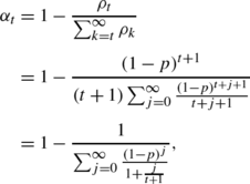
it is directly obtained that α t ≤α t+1 for all t=0,1,2,… , and
$$ \overset{\_}{\alpha}=\lim_{t\rightarrow\infty}\alpha_{t}=1-p. $$ -
(iib)
Take τ with a negative binomial distribution whose parameters are q and r, where 0≤q≤1 and r∈ℕ. In this case,

then
$$ \overset{\_}{\alpha}=\lim_{t\rightarrow\infty}\alpha_{t}=q. $$Moreover, it is verified that α t+1≤α t .
-
(iia)


Now, consider the Markov decision model (X,A,{A(x)∣x∈X},Q,c) and the performance criterion as

π∈Π, x∈X and \(\overset{\_}{\alpha}=\lim_{t\rightarrow \infty}\alpha_{t}\) (see Assumption 5.1). Let
Consider the following assumption.
Assumption 5.2
There exists a policy π∈Π such that v(π,x)<∞, for each x∈X.
Lemma 5.1
Suppose that Assumptions 4.2(a), 5.1, and 5.2 hold. Then J τ(x)≤V(x), x∈X.
Proof
By Theorem 4.2.3 in [8], there exists \(f\in\mathbb {F}\) such that
Iterating (19), it is obtained that
n≥1, x∈X, where
Q n(⋅∣x,f) denotes the n-step transition kernel of the Markov process {x t } when using \(f\in\mathbb{F}\). By Assumption 5.1, it results in
hence
n≥1, x∈X. Since V is nonnegative,
n≥1, x∈X. Letting n→∞ yields
□
Let \(f^{\ast}\in\mathbb{F}\) be the stationary optimal policy of the discounted problem and consider the following assumption:
Assumption 5.3
There exist positive numbers m and k, with \(1\leq k< 1/{\overset{\_}{\alpha}}\), and a function w∈M(X)+ such that, for all \((x,a)\in \mathbb{K}\),
-
(a)
c(x,a)≤mw(x), and
-
(b)
∫ X w(y)Q(dy∣x,a)≤kw(x).
Remark 5.2
-
(i)
Assumption 5.3 implies Assumption 4.2(b).
-
(ii)
Observe that
$$ E_x^\pi \bigl[ w(x_t) \bigr]\leq k^t w(x), $$(20)t=0,1,2,… and x∈X.
For t=0, (20) trivially holds, and for t≥1, using Assumption 5.3(b), it is obtained that
$$ E_x^\pi \bigl[w(x_t)\mid h_{t-1},a_{t-1} \bigr]=\int_X w(y)Q(dy \mid x_{t-1},a_{t-1})\leq kw(x_{t-1}). $$Taking expectations into account results in
$$ E_x^\pi \bigl[w(x_t) \bigr]\leq kE_x^\pi \bigl[w(x_{t-1}) \bigr]. $$(21)
Lemma 5.2
Under Assumptions 4.2(a), 5.1, and 5.3,
Proof
Firstly, observe that \(\sum_{t=0}^{\infty}(\overset{\_}{\alpha }^{t}-P_{t} )k^{t}\leq\sum_{t=0}^{\infty}(\overset{\_}{\alpha} k)^{t}< \infty\), since \(0<\overset{\_}{\alpha}k<1\) by Assumption 5.3. Then, under Assumption 5.3(a) and (20), for a stationary policy \(f\in\mathbb{F}\), it is obtained that

Taking f=f ∗, where f ∗ is the deterministic stationary optimal policy of the discounted problem, the proof is concluded. □
Let \(D_{n}:\mathbb{K}\rightarrow\mathbb{R}\) be the discrepancy functions defined as
Assumption 5.4
P(τ<+∞)=1.
Theorem 5.1
Under Assumptions 4.2(a), 5.1, 5.3, and 5.4,
x∈X and π∈Π.
Proof
For x∈X, by Lemma 5.2,

Now, for π∈Π and x∈X,

Observe that, for some positive integer M,

and by Assumption 5.4, \(\lim_{M\rightarrow\infty}\frac {P_{M+1}}{P_{n-1}}=0\). Then it is obtained in (23) that
Since α n−1≤1 and x=x n , it is obtained that
Finally, since \(v_{0}^{\tau}(\pi,x)=\jmath^{\tau}(\pi,x)\), and taking π=f ∗, (22) is obtained. □
6 Concluding Remarks
The results obtained in this paper permit working with discounted control problems with a varying-time discount factor, possibly depending on the state of the system and on the corresponding action as well. Besides, for MDPs taken into account in the article, i.e., MDPs with a total cost and a random horizon, it is possible to develop methods, as the rolling horizon procedure or the policy iteration algorithm, in order to approximate the optimal value function and the optimal policy.
References
Puterman, M.L.: Markov Decision Process: Discrete Stochastic Dynamic Programming. Wiley, New York (1994)
Baüerle, N., Rieder, U.: Markov Decision Processes with Applications to Finance. Springer, New York (2010)
Kozlowski, E.: The linear–quadratic stochastic optimal control problem with random horizon at the finite number of infinitesimal events. Ann. UMCS Inform. 1, 103–115 (2010)
Levhari, D., Mirman, L.J.: Savings and consumption with uncertain horizon. J. Polit. Econ. 85, 265–281 (1977)
Bather, J.: Decision Theory: An Introduction to Dynamic Programming and Sequential Decision. Wiley, New York (2000)
Chatterjee, D., Cinquemani, E., Chaloulos, G., Lygeros, J.: Stochastic control up to a hitting time: optimality and Rolling-Horizon implementation (2009). arXiv:0806.3008
Iida, T., Mori, M.: Markov decision processes with random horizon. J. Oper. Res. Soc. Jpn. 39, 592–603 (1996)
Hernández-Lerma, O., Lasserre, J.B.: Discrete-Time Markov Control Processes: Basic Optimality Criteria. Springer, New York (1996)
Guo, X., Hernandez-del-Valle, A., Hernández-Lerma, O.: Nonstationary discrete-time deterministic and stochastic control systems with infinite horizon. Int. J. Control 83, 1751–1757 (2010)
Hinderer, K.: Foundation of Non-Stationary Dynamic Programming with Discrete Time Parameter. Springer, New York (1970)
Bertsekas, D.P., Shreve, S.E.: Stochastic Optimal Control: the Discrete Time Case. Academic Press, Massachusetts (1978)
Author information
Authors and Affiliations
Corresponding author
Rights and permissions
About this article
Cite this article
Cruz-Suárez, H., Ilhuicatzi-Roldán, R. & Montes-de-Oca, R. Markov Decision Processes on Borel Spaces with Total Cost and Random Horizon. J Optim Theory Appl 162, 329–346 (2014). https://doi.org/10.1007/s10957-012-0262-8
Received:
Accepted:
Published:
Issue Date:
DOI: https://doi.org/10.1007/s10957-012-0262-8