Domain-driven co-location mining

Abstract

Co-location mining is a classical problem in spatial pattern mining. Considering a set of boolean spatial features, the goal is to find subsets of features frequently located together. It has wide applications in environmental management, public safety, transportation or tourism. These last years, many algorithms have been proposed to extract frequent co-locations. However, most solutions do a “data-centered knowledge discovery” instead of a “expert-centered knowledge discovery”. Successfully providing useful and interpretable patterns to experts is still an open problem. In this setting, we propose a domain-driven co-location mining approach that combines constraint-based mining and cartographic visualization. Experts can push new domain constraints into the mining algorithm, resulting in more relevant patterns and more efficient extraction. Then, they can visualize solutions using a new concise and intuitive cartographic visualization of co-locations. Using this original visualization approach, they identify new interesting patterns, and use uninteresting ones to define new constraints and refine their analysis. These proposals have been integrated into a prototype based on PostGIS geographic information system. Experiments have been done using a real geological datasets studying soil erosion, and results have been validated by a domain expert.

1 Introduction

Context

These last years, environmental monitoring has become an important research topic. The explosion of spatial data collected by experts, sensors and satellites opens new challenges and perspectives. Mining these spatial data to extract interesting, useful, and unexpected knowledge on environmental phenomenas is particularly challenging. For example, soil erosion has a deep impact all over the world, and affects environment and economy. This phenomenon is natural but it is greatly accelerated by anthropic activities (e.g. bush fires, deforestation, mining projects) and climate change (resulting in intense precipitation events). It has also a strong impact on connected terrestrial and coastal ecosystems such as mangrove and coral reefs. Identifying key components of these erosion processes is essential to have a good environmental management and a sustainable development.

Actual data volumes are considerable and their nature is complex (e.g. spatial, noisy, heterogenous). Understanding and predicting environmental phenomenons require advanced methods for data analysis and modeling. Mining spatial patterns, and more precisely co-locations, is one of the important topics when studying spatial data [15, 28, 29, 32, 51, 54, 55]. A co-location is a set of boolean features frequently occurring together [51]. An example of co-location in environmental data could be {m i n e, e r o s i o n}. This pattern highlights a possible correlation between mines and soil erosion. These last years, many algorithms have been proposed to extract frequent co-locations. However, interpretation of results by experts is difficult due to the huge number of patterns usually extracted (thousands to millions of patterns). Moreover, lots of these patterns are not really interesting for experts.

Challenges

Our work deals with the two following important challenges of knowledge discovery in data (KDD): how to improve the relevancy of extracted patterns? and how to facilitate interpretation of results by experts? These two challenges are closely related as we will show later in the paper.

Adding user constraints to improve pattern quality, or to express user requirements, has been widely studied in the itemset mining literature [42, 49]. Itemsets are a specific class of patterns. They represent sets of items that occur frequently in the same transactions. In the itemset setting, there is classically two approaches: integrating constraints in preprocessing or integrating constraints in the mining algorithm. One interest of the second approach is to iteratively integrate new constraints without needing to reprocess the data. Thanks to theoretical properties of some of these constraints, this second approach also enables to improve mining performances. Integration of expert constraints in pattern mining is not new, but it has never been done for spatial patterns, that exhibit specific properties compared with itemsets (s.t. spatial and thematic dimensions of geographical databases). In this context, our paper tackles the following questions:

• What kinds of constraints can be defined for co-locations, taking into consideration characteristics of spatial data and theoretical properties necessary to improve algorithm performances?

• How to help experts in choosing and defining their constraints?

Effective visualization of extracted patterns is one of the big challenges in KDD [13]. Lots of contributions have been done [8]. When working with spatial data, a classical approach is to display informations on maps. However, displaying a co-location on a map is not trivial because a co-location only represents a global spatial correlation between objects or events. For example, the co-location {m i n e, e r o s i o n} represents the correlation “soil erosion is often located near mines”. It is not associated to one location, since several mines and erosion objects can occur closely together in different locations. Considering that we may have thousands to millions of co-locations and for each one thousands to millions of instances, it is impossible to display all these objects on the map (it would become unreadable). However, it is important for experts to have a global view of the solutions before studying more precisely some patterns. As a consequence, our work have to solve the following problems:

• How to display a co-location on a map?

• How to display all extracted co-locations on a map in a concise and readable way for experts?

Contributions

To our knowledge, no contributions have tried to tackle these challenges. Most solutions do a “data-centered knowledge discovery” instead of a “expert-centered knowledge discovery”. Existing works focus on pruning techniques, spatial join optimization, local patterns or concise representations. They do not integrate experts knowledge and needs in the co-location mining process, nor a visualization approach adapted to expert practices (see Section 2).

To deal with these limits, we propose a new process where constraint-based mining and cartographic visualization of co-locations are combined to improve relevancy and interpretation of results. On the one hand, constraints decrease the number of patterns extracted, while increasing their relevancy, which facilitates visualization and interpretation of solutions. On the other hand, our effective visualization approach enables to quickly identify irrelevant patterns, which can be used by experts to define new constraints.

This process is based on a new family of spatial and thematic constraints exhibiting theoretical properties compatible with mining algorithms (see Section 4.2). In existing works, the only constraint integrated in the mining algorithm is the frequency constraint (to keep most frequent co-locations). Expert constraints are taking into account when selecting and preprocessing original data. As a consequence, data has to be reprocessed each time an expert needs to refine its analysis or change its constraints. Our approach avoids this problem. Experts can iteratively refine their analysis by integrating new constraints without reprocessing data. At each iteration, they obtain more meaningful co-locations, and algorithm performances are improved. Moreover, only constraints on data can be applied in preprocessing (e.g. filtering objects, features or themes from data). In our work, we propose new constraints on co-locations, which avoid analysis of uninteresting correlations for experts. So these constraints cannot be used in a preprocessing step, but during co-location mining.

Our process is also based on an original visualization approach for co-locations (see Section 4.3). This approach provides a concise and intuitive cartographic visualization of co-locations based on a new heuristic clustering algorithm. In existing works, the visualization of extracted co-locations is never covered. Restitution of solutions is done in a textual format (a basic report with a list of co-locations), which is not effective and does not correspond to expert practices. To the opposite, we propose a graphical representation of co-locations. In our approach, each co-location is displayed on the map depending on the spatial distribution of its instances. To limit the number of informations displayed on the map, we have developed a new effective clustering algorithm. Thus, our visualization approach provides to experts a concise and intuitive way to visualize results, while giving additional informations on co-locations (where and how they are generally located).

Finally, we have done an extensive experimental analysis of our approach on a real application (see Section 5). We studied soil erosion on two different areas. A qualitative analysis has been conduced by an expert. It shows the interest of our contributions to iteratively find more relevant patterns, and demonstrates how intuitive is our visualization approach. Our quantitative analysis illustrates the impact of the different parameters on performances, and shows the scalability of the whole process compared to existing approaches (i.e. the apriori-like co-location mining algorithm of Shekhar and Huang [51] and a visualization based on the two clustering algorithms of Ester et al. [19]; Pelleg and Moore [47]).

To sum up, the contributions of this paper are:

• 1. a generic process combining constraints and visualization to improve relevancy and interpretation of co-locations;

• 2. a new class of spatial and thematic constraints that can be integrated in any co-location mining algorithm;

• 3. a generic approach to optimize algorithm performances thanks to the theoretical property of these constraints;

• 4. a new visualization approach that provides a global view of extracted co-locations on a map;

• 5. an original and efficient clustering algorithm that summarizes informations displayed on the map;

• 6. a thorough application of the process on soil erosion data (with quantitative and qualitative analysis of results with an expert).

2 Related works

2.1 Spatial pattern mining

Spatial data exhibits a unique property: “everything is related to everything else but nearby things are more related than distant things” (first law of geography in Tobler [52]). In this context, spatial pattern mining aims at discovering implicit relations in spatial data using spatial proximity [27]. These approaches may be classified in three families: transactional approaches, multi-relational approaches and co-location-based approaches.

The principle of transactional approaches such as Koperski and Han [35]; Bogorny et al. [9] is to map spatial data to transactional data (such as in market basket analysis). Spatial relationships are extracted prior to pattern mining, and features are grouped into transactions. In other words, a transaction can be viewed as a set of features (e.g. mine, erosion, savanna) associated to the same zone (e.g. catchment basin). Thus, at the end of this preprocessing of spatial relationships, spatial information is no more explicitly encoded in the data. We have a classical transactional database. This preprocessing step enables to use classical frequent itemset mining algorithms. This method is used by Koperski and Han [35] to extract association rules in a geographic database given a spatial relationship (e.g. “objects near by large towns”). Bogorny et al. [9] extend the work of Koperski and Han [35] by introducing knowledge constraints in the preprocessing step.

Multi-relational pattern mining [14, 38, 40] extends transactional approaches to mine spatial databases composed of multiple tables. They also use inductive logic programming to express concept hierarchies and mine multi-level patterns in spatial databases. Spatial hierarchies represent geographic descriptions at different granularity levels (e.g. ward, district, county). Transactions materialize features (e.g. population, car availability) around reference objects (e.g. ward) and spatial relationships between objects (e.g. link to, close to).

Co-location-based approaches, also called event-based approaches, focus on events and their neighbor relationships [28, 51, 55]. They compute spatial relationships on-the-fly during extraction, and not in a preprocessing step such as in previous approaches. Shekhar and Huang [51] have defined the co-location concept based on Koperski and Han [35]. The goal is to find all subsets of spatial features likely to occur together. A new interest measure, the participation index, has been proposed to filter patterns. This measure is closely related to the cross-K function, a statistical measure of interaction between spatial objects. Thanks to the anti-monotone property of this predicate, a levelwise algorithm (an adaptation of the apriori algorithm of Agrawal and Srikant [1]) has been proposed to extract interesting co-locations. This co-location mining algorithm has been improved in Yoo and Shekhar [55] to avoid costly spatial joins in the database. Celik et al. [15] extend the notion of co-location to zonal co-location pattern (intuitively a local zone-scale co-location pattern). More recently, Qian et al. [48] propose an approach to mine co-location patterns w.r.t. several neighborhood constraints. Despite all of these contributions to co-location mining, to our knowledge, none of existing solutions integrate expert constraints in the mining process. They only propose a preprocessing step to filter input data w.r.t knowledge constraints.

Integration of expert constraints inside itemset mining algorithms is not new. In the literature, two classes of constraints have been used to filter itemsets: objective constraints and subjective constraints [42]. Objective constraints are generally based on frequency and/or statistical properties of itemsets. For example, the minimal frequency constraint [1] is such constraint. Subjective constraints enable to express interestingness of itemsets w.r.t. expert’s goals or needs (see, e.g., [44, 46, 49]). Examples of objective constraints for itemsets are: all items must be {=,≤,≥} to an expert value; a given value must (or mustn’t) be in the itemset; the size of the itemset must be smaller than a threshold; or the min/max/avg/sum of the numeric values in the itemset must be {=,≤,≥} to an expert value. Constraints proposed for itemset mining do not consider spatial or thematic aspects, which is normal since transactional data do not focus on these informations. To the opposite, organization of spatial data in thematic layers are key concepts of Geographical Information Systems. First, GIS were developed to store, manage, analyze and display geographical informations, in other words spatial data. Second, the notion of thematic layer was introduced by practitioners in order to organize and analyze informations based on logical layers. As a consequence, it is important to integrate these two aspects in co-location mining. It would enable experts to express operations that they usually do in a GIS (e.g. studying a specific area, or analyzing correlations between specific themes).

Let us recall that constraint-based mining enables to improve the relevancy of computed patterns, but also to use theoretical properties of constraints (e.g. monotonicity property) to perform complete though computationally efficient extractions (see, e.g., [10]). Thus, defining new constraints is not trivial since we have to ensure that their theoretical properties are compatible with mining algorithms.

2.2 Visualization of data mining results

Information visualization and data mining are two domains considered to achieve effective knowledge discovery [8]. Information visualization aims at helping interpretation of large quantity of data by providing effective visual representations. Data mining aims at extracting hidden knowledge in data by providing efficient algorithms. These two domains have been coupled in several papers. The literature review done in Bertini and Lalanne [8] identifies three types of visualization-mining cooperation: computationally enhanced visualization, visually enhanced mining, and integrated visualization and mining.

Computationally enhanced visualization corresponds to visualization approaches improved by data mining. For example, data mining (e.g. clustering or itemset mining) can be used to reduce informations displayed to users, which is a well known problem in visualization. As an example, Yang et al. [53] propose a hierarchical dimension ordering, spacing and filtering approach to explore high dimensional datasets. They group dimensions in a dimension hierarchy using a clustering approach. Thus, users can easily navigate and analyze the data. Morrison et al. [43] and Heer and Boyd [26] are other examples of such approaches based on multidimensional scaling and graph clustering.

Visually enhanced mining corresponds to data mining approaches where visualization techniques are used to provide easily understandable results to users. For example, MineSet [11] is an interactive system for data mining integrating data visualization. Different kinds of visualizer (statistics, scatter, map, tree) are available according to the type of result to visualize. Recently, Leung et al. [36] deal with visualization of frequent itemsets. The authors developed a system, WiFIsViz, for visualizing frequent itemsets based on orthogonal graphs (wiring-type diagrams). Frequent itemsets are shown in a two-dimensional space, where the x-axis shows items and the y-axis shows the frequencies (Fig. 1). An itemset X is represented by a horizontal line connecting nodes, where each node represents an item of X. Moreover, itemsets sharing the same prefix are merged, which improve the visualization.

Fig. 1

Examples of visually enhanced frequent itemset mining with WiFIsViz [36] and FP-Viz framework [34]

Integrated visualization and mining corresponds to approaches in which visualization and data mining are totally combined. In such solutions, human can directly interact with the mining algorithm using a visual environment. For example, Chen and Liu [16] propose a visual framework in which users can interactively evaluate and refine clustering at each step of the process. Andrienko et al. [4] also propose a visual analytics toolkit to analyze mobility data based on clustering. Thanks to this toolkit, users can progressively find and refine trajectory clusters through sampling and classification. Figure 2 shows an example of trajectories with the corresponding cluster.

Fig. 2

Example of spatial integrated visualization and mining to cluster cars trajectories [4]

As shown in the previous example, spatial data are usually displayed on a map since cartographic visualization is very intuitive for users. A typical system is the one proposed in Andrienko and Andrienko [3]. The user can perform different data analysis, such as clustering or association rules, and visualize the results on the map or a report. For example, after clustering, spatial objects are displayed on the map with different color and label w.r.t. their cluster. At the opposite, mined association rules are displayed in a textual report. When the mouse cursor is positioned on a specific rule of the report, the corresponding objects are highlighted in the map (and vice versa). More recently, Andrienko et al. [4] and Guo [23] also use a cartographic visualization to display large spatial data. They both use clustering and user interactions to limit informations displayed on the map. However, the first work study mobile objects trajectories, while the second one study geographically embedded networks (graphs).

As far as we know, none of the solutions proposed in the literature were designed to display co-location patterns in a simple, concise and intuitive way for experts. Existing solutions return results in a textual format. They do not take into consideration the spatial nature of the underlying objects and expert requirements. Initial works on visualization of co-location are presented in Selmaoui-Folcher et al. [50] and Desmier et al. [18].

3 Theoretical framework

3.1 Preliminaries and definitions

This section recalls the co-location mining framework proposed in Shekhar and Huang [51]; Huang et al. [28]; Yoo and Shekhar [55]. Let $\mathcal {F}$ be a set of features (also called object-types) and $\mathcal {D}$ be a database of spatial objects. Each object in $\mathcal {D}$ consists of a tuple < o b j e c t_i d, l o c a t i o n, f e a t u r e>, where $feature \in \mathcal {F}$. We denote that each object is associated with a feature $f \in \mathcal {F}$ by $f_{object\_id}$. For example, in Fig. 3, $\mathcal {F} = \{A,B,C,D,E\}$, $\mathcal {D}=\{ A_1,C_2,B_3...,E_{12}\}$ with A ₁ = < 1, (x ₁, y ₁),A>, C ₂ = < 2, (x ₂, y ₂),C>, etc.

Fig. 3

Example of spatial database

A co-location $X \subseteq \mathcal {F}$ is a subset of features (object-types) such that its instances are located in the same neighborhood. The neighborhood relationship is defined as a binary relation $\mathcal {R}(o,o')$ between two spatial objects o and o ^′. Depending on user requirements, $\mathcal {R}$ can be based on a distance threshold between two objects, or based on their intersection, or it can be any reflexive and symmetric spatial relation (e.g. the inclusion relation does not satisfy these properties). A co-location instance is a set of objects that forms a clique under $\mathcal {R}$. To simplify, we use in our examples a simple neighborhood relation based on the Euclidean distance (i.e. two objects are neighbors if their Euclidean distance is less than a given threshold). For example (Fig. 3), the set of objects {A ₉, B ₄, D ₁₀} is an instance of the co-location {A, B, D} w.r.t. a fixed Euclidean distance threshold (represented by dotted lines). To the opposite, {A ₁, B ₄, C ₇} or {A ₁, B ₄, D ₁₀} are not co-location instances of {A, B, D}. Note that an instance I of a co-location X is a set of objects such as no proper subset of I is also a co-location instance (we cannot have {A ₀, A ₁, B ₄, C ₇}). The table instance of a co-location X, denoted T I _X , is the set of all its instances. For example, the table instance of {A, B, C} is T I _{{A, B, C}}={{A ₁, B ₈, C ₇},{A ₅, B ₆, C ₂}} and the table instance of {B, D} is T I _{{B, D}}={{B ₄, D ₁₀}} (see Fig. 3).

However, not every co-location is interesting. Thus, authors have proposed a prevalence measure to determine the strength (the frequency) of a co-location. This measure is called participation index and it represents the minimal probability to have an object in a given co-location instance compared with the total number of instances. More precisely, they introduce the participation ratio p r(X, f) for a feature f in a co-location X as the fraction of objects with feature f in instances of X, to the total number of objects with feature f. For example, in Fig. 2, p r({A, B, C},A)=2/3 since {A, B, C} has two instances (T I _{{A, B, C}}={{A ₁, B ₈, C ₇},{A ₅, B ₆, C ₂}}) and feature A has three instances (A ₁, A ₅ and A ₉). In the same way, p r({A, B, C},B)=1/2 and p r({A, B, C},C)=1. Then, they define the participation index, denoted p i(X), as the minimum of the participation ratios. In the example, p i({A, B, C})= m i n(p r({A, B, C},A), p r({A, B, C},B), p r({A, B, C},C)) =1/2.

Based on these definitions, we have to solve the following problem : Given $\mathcal {F}$ a set of features, $\mathcal {D}$ a spatial database, $\mathcal {R}$ a neighbor relation and α ∈ [0, 1] a threshold. The problem is to find the set of prevalent co-locations, i.e. $\{X \subseteq \mathcal {F} | pi(X) \ge \alpha \}$.

3.2 A new framework for constraint-based co-location mining

In this subsection, we extend the co-location concept based on the theoretical framework of Mannila and Toivonen [41]. Thus, classical co-location mining is generalized to extraction of co-locations based on any monotone domain constraint.

The pattern mining framework defined in Mannila and Toivonen [41] is a generalization of the frequent itemset mining problem [2]. Thanks to this framework, itemset mining algorithms have been successfully applied in various domain such as association rules [1], functional dependencies [30], inclusion dependencies [17], and query rewriting [33] to mention a few. This framework can be summarized as follows: “Given a database $\mathcal {D}$, a finite language $\mathcal {L}$ for expressing patterns or defining subgroups of the data, and an anti-monotone (or monotone) predicate Q for evaluating whether a pattern $\varphi \in \mathcal {L}$ is true or “interesting” in $\mathcal {D}$, the discovery task is to find the theory of $\mathcal {D}$ with respect to $\mathcal {L}$ and Q, i.e. the set $Th = \{\varphi \in \mathcal {L} | Q(\mathcal {D},\varphi ) \text { is true}\}$”. The co-location mining problem defined in Shekhar and Huang [51] is another application of this framework. Thus, it benefits of the great amount of work done to develop itemset mining algorithms. It explains why Shekhar and Huang [51] could easily adapt the classical A p r i o r i algorithm [1] (initially proposed for frequent itemset mining) to mine co-location patterns.

Fitting co-location mining in this framework has another advantage: we can generalize the discovery of co-location patterns to any anti-monotone boolean predicate Q and to any boolean spatial relationship $\mathcal {R}$. The mapping of the co-location concept in the previous framework, and its extension to a domain driven co-location framework is presented in Fig. 4.

Fig. 4

Domain-driven co-location mining framework

This extension also provides a condensed representation of the co-locations: the positive border of interesting co-locations (i.e. maximal interesting co-locations w.r.t. set inclusion). Indeed, since any subset of an interesting co-location is also an interesting co-location (thanks to the anti-monotone property), experts can deduce all the interesting co-locations based on the maximal ones. In practice, the number of interesting co-locations may be extremely important. Only providing maximal interesting co-locations to experts might make easier their interpretation of results.

4 Combining constraints and visualization to deliver domain knowledge

4.1 Overview of the process

In this paper, we propose a new process where constraint-based mining and cartographic visualization of co-locations are combined to improve relevancy and interpretation of results. This process, derived from the classical KDD process of Fayyad et al. [20] is illustrated in Fig. 5. This process begins with the classical steps of KDD, i.e. data selection, data preprocessing and data transformation. Then, constraint-based co-location mining is performed based on expert parameters (i.e. frequency threshold and domain constraints). In the first iteration of the process, the set of domain constraints may be empty if the expert doesn’t have enough knowledge about the studied phenomenon. After, extracted co-locations are displayed on a map thanks to our cartographic visualization approach. Based on the generated map, the expert identify interesting patterns leading to new knowledge, but also uninteresting patterns. These frequent irrelevant patterns are used by the expert to express new spatial and thematic constraints. These new constraints are used in the next iteration of the process to refine co-location mining. Note that at this moment, the expert can also decrease the frequency threshold to find other, less frequent, patterns.

Fig. 5

Our KDD process combining constraints and visualization to improve relevancy and interpretation of co-locations

4.2 Domain-driven extraction of co-locations

4.2.1 Spatial and thematic domain constraints

In the previous framework, the conjunction of anti-monontone constraints, C _{D o m} , is used to integrate domain constraints in the mining process. This section presents several domain constraints that can be used by experts to integrate their knowledge. This approach leads to a better interpretation of results, and improve algorithm performance by pruning non relevant information during the mining process. Note that this work differs from Bogorny et al. [9] in which knowledge constraints are introduced in a preprocessing step.

In our context, domain constraints represent known, or unrelevant, relations for experts. These constraints can be considered as exclusion rules. We define two types of constraints :

• constraints on features and themes

• spatial constraints on objects

Constraints on features and themes

The first type of constraints excludes co-locations w.r.t. specific features and/or themes. The idea here is to avoid analysis of uninteresting correlations.

Several constraints can be expressed based on this principle. The most basic one is to exclude user-defined features from co-locations. In other words, given a co-location $X \subseteq \mathcal {F}$ and a set of features $F \subseteq \mathcal {F}$, the predicate C _{a l l F e a t u r e s} (X, F)=¬(F⊆X) is true iff the features of F are not in the co-location X. For example, if F={s e r p e n t i n i t e, h a r z b u r g i t e}, then all co-locations composed of {s e r p e n t i n i t e, h a r z b u r g i t e} are ignored during pattern mining. In the same way, we can define the predicate C _{f e a t u r e s} (X, F)=¬(F∩X≠∅), which is true if none of the features of F are in the co-location X.

In domains manipulating geographical data, Geographical Information Systems (GIS) are classical tools used by experts to store and study their data. A key concept of GIS is the organization of data in thematic layers. Arctur and Zeiler [5] defined a thematic layer as “a collection of common geographic elements, such as road networks, soil types, an elevation surface ...”. The notion of thematic layers was introduced by practitioners in order to organize the geographic informations in maps into logical information layers. This concept is a key element in the manipulation and analysis of data by practitioners.

To extend domain constraints to themes, we need to define more formally the notion of themes.

Definition 1

Given $\mathcal {F}$ the set of features, a theme t is a set of features such that $t \subseteq \mathcal {F}$.

Remark 1

In a GIS, the set of all themes, denoted $\mathcal {T}hemes$, is such that $\forall t_1, t_2 \in \mathcal {T}hemes$, t ₁∩t ₂=∅.

Based on this definition, we can define another predicate that excludes co-locations related to a given theme. More formally, given a co-location $X \subseteq \mathcal {F}$ and a theme $t \in \mathcal {T}hemes$, the predicate C _{t h e m e} (X, t)=¬(X∩t≠∅) is true iff the co-location X is not composed of theme t features. For example, if t={savanna, sparse vegetation on ultramafic substrate, woody-herbaceous scrub, woodland dense scrub, forest on ultramafic substrate } is the vegetation theme, all co-locations related to the vegetation theme, such as {s a v a n n a, b a r e s o i l, s e r p e n t i n i t e}, are not studied.

More generally, we can identified two types of domain constraints: intra-theme constraints and inter-theme constraints. Intra-theme constraints exclude relations (and thus co-locations) between features from the same theme. For example, the expert may not be interested in relations between features serpentinite and harzburgite in the lithology theme. It is the case if the expert doesn’t want to study correlations between different soil types. Inter-theme constraints exclude relations between features of several specific themes. For example, the expert may not be interested in relations between hillslope erosion and mines in erosion theme and human constructions theme. It is the case if the expert wants to focus its study on natural erosion.

For intra-theme constraints, we can define a predicate that excludes co-locations showing correlations related to a given theme. More formally, given a co-location $X \subseteq \mathcal {F}$ and a theme $t \in \mathcal {T}hemes$, the predicate C _{i n t r a} (X, t)=¬(|X∩t|≥2) is true iff the co-location X is not composed of several features of theme t. For example, if t={savanna, sparse vegetation, woody-herbaceous scrub, woodland dense scrub, forest on ultramafic substrate } is the vegetation theme, the co-location {s a v a n n a, s p a r s e v e g e t a t i o n} is not studied (as well as all its supersets), whereas the co-location {s a v a n n a, b a r e s o i l} is extracted.

For inter-theme constraints, we can extend previous constraints to detect co-locations based on several themes. The predicate C _{i n t e r} (X, t ₁, t ₂)=¬((X∩t ₁≠∅)∧(X∩t ₂≠∅)) is true iff the co-location X is not composed of features in themes t ₁ and t ₂. Such constraint is useful if experts want to avoid analysis of correlations between themes t ₁ and t ₂. More generally, given a co-location $X \subseteq \mathcal {F}$ and a set of themes $T \subseteq \mathcal {T}hemes$, the predicate C _{i n t e r} (X, T)=¬(∀t∈T(X∩t≠∅)) is true iff all the themes of T are not studied in the co-location X. For example, if T={v e g e t a t i o n, l i t h o l o g y}, then all co-locations based on the vegetation and the lithology themes, such as the co-location {s a v a n n a, s e r p e n t i n i t e, h a r z b u r g i t e}, are not studied (s a v a n n a∈v e g e t a t i o n and s e r p e n t i n i t e, h a r z b u r g i t e∈l i t h o l o g y ). Note that patterns such as {s a v a n n a, s p a r s e v e g e t a t i o n, b a r e s o i l} are still extracted, since b a r e s o i l isn’t related to a theme of T.

The previous constraint enables experts to prune patterns fully related to specific themes. For example, if T={vegetation, lithology, man-made construction }, the co-location {s a v a n n a, s e r p e n t i n i t e, h a r z b u r g i t e} is studied, because the co-location doesn’t deal with the man-made construction theme. To cope with such case, we introduce the predicate C _{p a r t I n t e r} (X, T)=¬(∃t ₁∈T(t ₁∩X≠∅)∧∃t ₂∈T(t ₂∩X≠∅)), which is true iff co-location X is not related to themes of T (not necessarily all themes, but at least 2). Thus, this predicate enables to prune all co-locations related to T themes, even if only a subset of T themes match. We call such constraints partial inter-theme constraints. With such constraint, if T={vegetation, lithology, man-made construction }, the co-location {s a v a n n a, s e r p e n t i n i t e, h a r z b u r g i t e} is not studied.

Table 1 presents all constraints on features and themes. One interest of our approach is that new domain constraints can be defined based on a conjunction, or disjunction, of the previous ones. For example, we can define the predicate C _{i n t e r} (X, F, t)=C _{f e a t u r e s} (X, F)∧C _{t h e m e} (X, t), which is true iff co-location X does not study the relation between F features and theme t.

Table 1 Constraints on features and themes C _{D o m}

All the constraints defined in this section are anti-monotone, and can be used to prune the search space. The proof of monotonicity is straightforward for basic constraints. For example, given a theme t (a set of features), if X is a set of features satisfying C _{i n t r a} (X, t), i.e. |X∩t| < 2, then any subset Y of X also satisfies C _{i n t r a} . For more complex constraints such as conjunction/disjunction of constraints, the predicate stills anti-monotone since each of the basic constraints is anti-monotone. For example, let X be a co-location and C, C ^′ be two basic constraints on features and themes. If X satisfies the constraint C∨C ^′, Y⊆X also satisfies this constraint, since C and C ^′ are both anti-monotone.

Spatial constraints on objects

The second type of constraints excludes spatial objects. The idea here is to avoid analysis of specific correlations in user-defined geographical areas. For example, such constraint can be used by experts to focus their study on a specific area. On the contrary, it can be used to exclude an area for which experts know that there is noisy data.

An example of such constraint could be “study only objects located in the rectangular area delimited by (100,200,400,600) coordinates”. More formally, let $\mathcal {D}$ be the geographical database, $I\subseteq \mathcal {D}$ be an instance of a co-location X and shape be the geographical coordinates of a polygon. The predicate C _{s p a t i a l I n} (I, s h a p e)=(∀o∈I(I n(o, s h a p e))) is true iff all objects of a co-location instance I are in the shape area.

This basic constraint can be generalized to any spatial boolean relation r. The predicate C _{s p a t i a l A l l} (I, s h a p e, r)=(∀o∈I(r(o, s h a p e))) is true iff all objects of instance I satisfy the spatial relation r in the area shape. Thanks to this predicate, it is possible to express constraints such as “study all instances whose objects are near a mine area”. Note that all objects in I must satisfy the spatial relation. For example, if r is the relation “not in”, all objects in I must not be in the area shape. An instance that has only some of its objects not in the area is not studied. Indeed, a spatial constraint such as “ ∃o∈I(r(o, s h a p e))” cannot be used because, in such case, the participation index of co-location X may be greater than the one of Y⊆X, which is the basic property used to prune the search space in the mining algorithm.

Spatial constraints can also be mixed with feature and theme constraints. Such constraint can be used to avoid analysis of specific correlations in specific areas. An example of this type of constraints could be “do not study objects characterized by not bare ground or vegetation theme, and located in a rectangular area having (100,200,400,600) as coordinates”. In this example, the predicate is C _{s p a t i a l A l l} (I, s h a p e, n o t I n)∧C _{f e a t u r e s} (X,{n o t b a r e g r o u n d})∧C _{t h e m e} (X,{v e g e t a t i o n})with I aninstance of co-location X and s h a p e = < (100,200), (400,200), (400,600), (100,600)>.

Table 2 presents all spatial constraints. Such as for thematic constraints, new domain constraints can be defined using a conjunction/disjunction of these spatial constraints. For example, experts can focus on correlations between a mine and its nearby environment using a constraint such as C _{m i n e} (I, s h a p e M i n e)= C _{s p a t i a l A l l} (I, s h a p e M i n e, i n)∨C _{s p a t i a l A l l} (I, s h a p e M i n e, n e a r). This spatial constraint enables to only study instances whose objects are in the perimeter of the mine or close to it.

Table 2 Spatial constraints C _{S p a}

On the contrary to constraints on features and themes, spatial constraints are not used directly to prune co-locations. These constraints affect the computation of the co-location ratio by reducing the number of co-location instances studied. Thus, they are not involved in the predicate $\mathcal {Q}$ used in the co-location mining algorithm, but in the table instance calculation. Therefore, the definition of table instance is modified. The table instance T I _X of a co-location X in spatial database $\mathcal {D}$ is:

$$\begin{array}{@{}rcl@{}} TI_X & = &\{I \subseteq \mathcal{D} \mid~\text{I is an instance of X according to}~\mathcal{R}~and~C_{Spa}(I) = true \} \\ & & \text{with}~C_{Spa}(I)~\text{is any conjunction/disjunction of spatial constraints} \end{array} $$

Note that these spatial constraints do not modify the anti-monotonicity of the co-location predicate. Indeed, the number of instances used to process the participation index is always decreasing (not strictly) whenever we have a conjunction or disjunction of the previous spatial constraints. For example, given shape, s h a p e ^′ two areas and r, r ^′ two spatial boolean relations. If I is an instance of X satisfying a conjunction of spatial constraints C _{s p a t i a l A l l} (I, s h a p e, r)∨C _{s p a t i a l A l l} (I, s h a p e ^′, n e a r ^′), J⊆I is also an instance of Y⊆X, since ∀o∈I, we have r(o, s h a p e) or r(o, s h a p e ^′).

4.2.2 Mining co-locations using domain constraints

Thanks to the pattern mining theoretical framework, the domain constraints introduced in the previous subsection can be directly integrated in pattern mining algorithms. In this subsection, we present how our constraints can be integrated in two existing pattern mining algorithms: a levelwise apriori-like algorithm [1, 41, 51] and an adaptive algorithm [21]. These two algorithms highlight the generic nature of our approach.

A levelwise algorithm for finding all constrained co-locations

A classical approach to mine patterns is to use a levelwise exploration of the search space. More precisely, the principle of this approach is to do a breadth-first exploration of the search space from smaller patterns to larger ones, and to use an anti-monotone property of the predicate to prune patterns. Indeed, if the pattern X is false w.r.t. the predicate, all patterns Y⊃X are false.

First, the algorithm searches interesting patterns of size 1. Then, at each iteration k, a set of candidate patterns of size k, denoted C a n d _k , is generated by using interesting patterns of size k−1. A candidate pattern is a pattern having all its k−1 sub patterns interesting. After this generation step, all candidate patterns are tested against the predicate, and the resulting interesting patterns are used to begin the next iteration (others are pruned). The algorithm stops when the set of candidate patterns is empty.

and Toivonen [41], and used in Shekhar and Huang [51] for co-location mining, is modified as follows:

As shown by Algorithm 1, spatial constraints on objects are used in the evaluation step (lines 4-8), i.e. when testing if a co-location is interesting or not w.r.t. the participation index threshold. Actually, these constraints limit the number of objects studied during the generation of the table instance of each co-location (line 5), and thus limit the number of spatial joins done. Constraints on features/themes are used in the generation step (line 11), i.e. when constructing new candidate co-locations based on interesting ones found in the previous iteration. These constraints remove, from the set of candidate patterns, co-locations that are not satisfying thematic constraints defined by the expert.

An adaptive algorithm for finding maximal constrained co-locations

A classical levelwise strategy is efficient when the size of interesting patterns remains small. However, when the dataset has large interesting co-locations, the search space explored by such strategies is exponentially large (2^k co-locations for an interesting co-location of size k), and the algorithm does not fit in memory. To avoid such problem, several strategies have been proposed in the literature (e.g. depth-first strategies in Zaki et al. [56], Burdick et al. [12], levelwise exploration with “jumps” in Bayardo [7]; Lin and Kedem [37], pattern growth strategies in Han et al. [25]).

In this paragraph, we present an adaptive strategy based on the work done in Flouvat et al. [21] for maximal frequent itemset mining. The principle of this strategy is to combine the strength of both levelwise algorithm and dualization based algorithms, to find maximal co-locations. “Small” maximal interesting co-locations are efficiently discovered using the levelwise strategy. “Large” maximal interesting co-locations are efficiently discovered by dualization. A dualization corresponds to a jump into the search space, where “small” uninteresting patterns (discovered by the levelwise algorithm) are used to generate large potentially interesting patterns. These “jumps” are not based on a heuristic such as in many algorithms, but they are based on a theoretical property of the positive and negative borders [45].

Recall that another interest of mining maximal interesting co-locations is to provide a condensed representation of all interesting co-locations, since this set is smaller and experts can deduce all interesting co-locations based on maximal ones (but not their interestingness measure). When the number of interesting co-locations is too large, this makes easier interpretation of results by experts.

This algorithm does a levelwise generation (lines 2 and 24) and evaluation (lines 5–12) of candidate co-locations. Such as in the previous levelwise algorithm, domain constraints are used in these steps to prune candidate patterns (in red, lines 1,2 and 24) and to prune spatial objects (in red, line 6 and 17). In line 13, maximal constrained co-locations found during this levelwise exploration are stored in the positive border B d ⁺. The levelwise exploration also finds (minimal) uninteresting co-locations (line 10). These uninteresting co-locations are used to do a dualization/jump in the search space (lines 15–22), and to generate large potentially interesting co-locations. The theoretical properties of dualization guarantee that these patterns are the best maximal potentially interesting co-locations that can be generated based on known co-locations. Co-locations of this “optimistic” positive border are evaluated against domain constraints and participation index (line 17 and 18). Maximal constrained co-locations found are stored in the positive border (line 19). They are also used to prune candidate patterns in the levelwise generation step (line 24). This alternation of levelwise exploration and jumps continues until no more candidate patterns are generated. Note that jumping too soon may not be interesting, since we may not have enough informations (known interesting co-locations) to generate maximal interesting co-locations. To deal with this problem, the function I s D u a l i z a t i o n R e l e v a n t is used to find the best level to begin jumps w.r.t. dataset characteristics (see Flouvat et al. [21] for more details).

4.3 Domain-driven visualization of co-locations

The visualization of data mining results is essential to have usefull domain knowledge. In domains manipulating geographical data, GIS are classical tools for storing and visualizing spatial data. A main characteristic of GIS is the cartographic visualization of the information in thematic layers.

However, the potential high number of co-locations and instances may lead to an unreadable map. Moreover, if co-locations are presented in a textual report, experts lose spatial information of the underlying objects (see Fig. 6). Another option is to display all instances of only one selected co-location. This approach is done by Andrienko and Andrienko [3]. It enables to have detailed informations about events of one preselected co-location, but we can’t have a global view of all co-locations at the same time.

Fig. 6

Co-location visualization problem

To deal with these problems, we propose a new cartographic visualization of co-locations in a GIS. Since each interesting co-location may have a high number of instances, our idea is to summarize these instances using a new clustering approach, and to integrate them in a layer of the GIS. The resulting co-location layer will display to experts where and how each co-location is generally located, thus giving a global view of the spatial distribution of the solutions.

Thus, if we refer to the classification done in Bertini and Lalanne [8], we present in this paper a visually enhanced mining approach. Visualization techniques are used to provide easily understandable data mining results to users. However, our approach differs from basic approaches using only classical visualizer (e.g. scatter, map, trees), since it uses data mining (clustering) to improve map readability.

4.3.1 How to visually represent a co-location?

First of all, we introduce the visual representation of co-locations proposed in this paper. As introduced in Section 3, co-location instances are sets of objects that form cliques under a neighborhood relation. As a consequence, it is natural to represent each co-location by a labeled clique, where each vertex is a feature and each edge represents the neighborhood relation. Figure 7 illustrates this definition (without considering colors).

Fig. 7

Colored and labeled clique representation of co-location {m i n i n g z o n e, s p a r s e v e g e t a t i o n, s e n s i t i v e t r a i l, r i v e r e r o s i o n} with p i({m i n i n g z o n e, s p a r s e v e g e t a t i o n, s e n s i t i v e t r a i l, r i v e r e r o s i o n})=0.8

An important aspect in co-location mining is the prevalence measure (i.e. the participation index). We use edge-coloration to visually represent the strength of a co-location. We let users choose a “base color” for all edges. Then, for a given co-location, color of edges is a saturation adjustment based on this color. The color saturation is calculated using the prevalence measure (saturation factor). A strong co-location (i.e. with a high value of participation index) will have a bright color, whereas a weak co-location will have a darker one. For example, in Fig. 7, the base color chosen by users is red and edges color is bright red since the participation index of the co-location is high.

A main characteristic of GIS is a cartographic visualization of data in thematic layers (e.g. vegetation, erosion or man made construction), each one being composed of spatial objects associated to features/attributes (e.g. tropical forest, savannah or maquis for the vegetation theme). In our approach, we use vertex-coloration to show the theme associated to each feature. For example, in Fig. 7, vertex color for “sparse vegetation” is green since this information belongs to the “Vegetation” layer of the GIS.

4.3.2 How to position co-locations in the GIS map?

Clustering the spatial distribution of a co-location

A co-location only gives in itself few spatial informations. For example, saying that “co-location {A, B, C} is frequent” only informs the experts that object-type A, B and C are often close to each other, but he don’t know where and how. The spatial information of a given co-location is mainly carried by its instances. Since the number of instances of a given co-location may be huge and their spatial distribution heterogeneous, we have to identify some typical localizations, i.e. to group instances w.r.t. their spatial position. To do this, we perform a cluster analysis.

This cluster analysis can be done using any clustering method such as K-means [39] or DBSCAN [19], directly in the mining algorithm. For each candidate co-location X, the mining algorithm generates its table instance to process the participation index. If the constraints are satisfied, the candidate co-location is interesting and the clustering can be applied on the table instance. This can be done during the evaluation step (for example, line 6 in Algorithm 1).

However, running a new clustering for each co-location is time consuming. We can optimize this processing by considering that all co-locations are constructed based on the same set of features. Therefore, we develop a two-steps heuristic clustering method integrated in the mining algorithm based on:

• a clustering of each feature instances, run once at the beginning of the co-location mining algorithm (Algorithm 3).

• a clustering of each co-location instances based on the preprocessed clusters, using a merge and split approach (Algorithm 4).

  

  

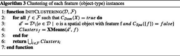
First, Algorithm 3 generates clusters of each feature instances as a preprocessing step for co-location mining. In other words, it summarizes where each object-type (feature) occurs. For each feature f satisfying domain constraints (line 1), the algorithm groups objects having feature f based on their locations (line 3–4). Note that only objects satisfying spatial domain constraints are studied (line 3). These clusterings are done using the X-means algorithm [47] implemented in Weka [24]. The interest of X-means compared to K-means is that the number of clusters k is no more an input parameter. Figure 8 (step “pre processing clusters”) illustrates this “pre-clustering” in which instances of each object-type (e.g. A, B and C) are partitioned independently.

Fig. 8

Clustering instances of co-location {A, B, C}

Second, Algorithm 4 uses these preprocessed clusters as a basis for clustering the table instance of each interesting co-location. This algorithm is used in line 7 in the levelwise Algorithm 1, and lines 13 and 19 in the adaptive Algorithm 2. It processes each table instance using a merge and split approach. Given a co-location X, its table instance T I _X and the clusters of X’s features $\bigcup _{i\in {X}} Clusters_i$, this methods partitions T I _X ’s instances using preprocessed clusters of i∈X. The principle is to partition (“split”) instances according to the features f having the highest number of clusters. However, using this method, we may have conflictual clusters, i.e. two different clusters sharing common objects. Figure 8 illustrates this problem for co-location {A, B, C}. If we split according to clusters of C, we have {A ₂, B ₂, C ₂} and {A ₃, B ₂, C ₃} (two instances of co-location {A, B, C}) in two different clusters. However, these two clusters share a common object: B ₂. This means that these two clusters are not so far from each other. To deal with this problem, we study each pair of objects o1 and o2 in different clusters of f∈X, denoted by c l u s t e r _o1 and c l u s t e r _o2 (lines 4-8). These objects are in two instances I ₁ and I ₂ of co-location X. If these instances share a common objects o ^′ with feature g∈X (g≠f), then c l u s t e r _o1 and c l u s t e r _o2 are conflictual clusters (line 8). In such case, c l u s t e r _o1 and c l u s t e r _o2 are merged (line 9). We continue this merge approach until the features f having the highest number of clusters does not change anymore (line 13). Then we can split instances of X w.r.t. clusters of f (line 14). In the example of Fig. 8, this approach results in merging the two first clusters of C.

From clusters of instances to co-locations in the GIS map

For each interesting co-location X, at the end of the clustering step, we have several clusters of instances representing the typical locations of X. For example, we have three typical locations (i.e. three clusters) for co-location {A, B, C} in Fig. 8. We propose to associate each typical location (i.e. each cluster) to a clique, and to position the vertices of the clique based on the spatial coordinates of the objects in the cluster.

A co-location X is set of features (or object-types). As presented in Section 4.3.1, each feature f∈X is associated to a vertice in the clique visual representation. Thus, for a given cluster (i.e. a typical location), the position of each feature f in the map (i.e. the position of the vertice with label f) is the average position of the objects associated to this feature in the cluster. In other words, each vertex with feature f is the centroid of f’s objects in the studied cluster. For example, in Fig. 9, the first cluster is composed of four instances of co-location {A, B, C}. These four instances involve 4 objects with feature A ({A ₁, A ₂, A ₃, A ₄}), 3 objects with feature B ({B ₁, B ₂, B ₃}), and 3 objects with feature C ({C ₂, C ₃, C ₄}). To represent this typical location of co-location {A, B, C}, we draw in the map a clique having 3 vertices (one with label A, one with label B and one with label C). Each vertex is the centroid of the objects with the corresponding feature (e.g. the vertex with label A is the centroid of objects {A ₁, A ₂, A ₃, A ₄}).This approach is applied to the three clusters of {A, B, C}, resulting in three cliques in the final map.

Fig. 9

Visualization of a co-location {A, B, C} in the GIS Map

The main interest of this approach is to visualize more precisely where and how interesting co-locations are generally located. Thus, it gives additional informations to experts compared with existing solutions. For example, Fig. 9 shows that co-location {A, B, C} is generally located in the north west, in the center and in the south east of the map. This approach has the advantage to provide experts a global picture of the spatial distribution of all co-locations. Using a classical visualization approach, it would have been difficult to have such informations. Note that this approach can also give additional informations on how features of a co-location are compared to each others.

5 Application to soil erosion data

5.1 Prototype architecture

The proposals discussed in this paper have been integrated in a prototype coupled with a PostGIS database (Fig. 10). PostGIS is a spatial database extension for PostgreSQL.

Fig. 10

Architecture of the prototype

For the data mining part, this prototype is based on a data mining tool called iZi [22]. This tool is used to solve interesting pattern mining problems as defined in the formal framework of Mannila and Toivonen [41], by providing generic algorithm implementations. This tool has been extended by two sub-modules. The first one allows to mine interesting co-locations. It takes as input parameters the data (a PostGIS table), the spatial relation studied, the participation index threshold used to select interesting co-locations, and the expert constraints. This module can output all interesting co-locations or only the maximal ones. The second one allows the access and storage of co-locations in a PostGIS geographical database.

For the visualization part, Q u a n t u m G I S (a free desktop application framework) is used as an interface to visualize data and interesting co-locations stored in the GIS. Note that experts can use the zoom functionality of the GIS to focus on an area or on specific patterns.

The co-location mining module extracts interesting co-locations w.r.t. domain constraints, generates spatialized clique representations and stores theme in a PostGIS table. Then, results are displayed to experts by Q u a n t u m G I S. Experts can choose to display several thematic layers among them one for interesting co-locations.

5.2 Experimental protocol

We used our approach to study soil erosion in two areas. These two areas are located in the south east coast of New-Caledonia. In these areas, natural erosion takes place as well as erosion related to mining activities. The first area is the Ouinné area. Its surface is about 110 k m ². 18 thematic layers were considered. Among them are thematic layers dealing with soil erosion, land cover, geological surfaces, mining activities and road network. These layers contain 68 features (object-types) and 3943 spatial objects. The second area is the Kwe Binyi area (which is located 50 km south east from Ouinné). Its surface is about 29 k m ². In this dataset, 21 thematic layers were considered. These layers contain 71 features (object-types) and 7306 spatial objects.

The data was stored in a PostGIS geographical database (vector format). Two spatial relations of PostGIS were considered to define the neighborhood relationship: the S t_i n t e r s e c t s function and the S t_d w i t h i n function. With the first one, two objects are neighbors if their spatial intersection is not empty (i.e. they share at least a boundary). With the second one, two objects are neighbors if they are within a distance of one another (two distance thresholds are studied). We focus our analysis on maximal interesting co-locations (w.r.t. vertex inclusion), with a size strictly greater than one.

First, a specialist in soil erosion analyzes results of the apriori-like co-location mining approach of Shekhar and Huang [51] on the Ouinné dataset. This approach does not consider domain knowledge (i.e. experts constraints). Several participation index thresholds were studied with the spatial relations based on S t_i n t e r s e c t s and S t_d w i t h i n PostGIS functions. We used our clustering-based visualization approach to display interesting co-locations to the expert. This highlights the interest of our visualization approach.

Then, the expert analyzes results of our constraint-based co-location mining approach. The constraints were defined using uninteresting patterns (known or irrelevant co-locations) found by the expert in the previous experiments (without constraints). The main objective of this analysis is to highlight that new interesting patterns can be discovered thanks to our constraints.

After this qualitative analysis, we study the performances of our approach, compared with existing ones, on the Ouinné and Kwe Binyi datasets. We compare our constraint-based co-location mining with the apriori-like co-location mining algorithm of Shekhar and Huang [51]. We also compare our new clustering algorithm, used in our visualization approach, with the DBSCAN algorithm of Ester et al. [19] and the X-Means algorithm of Pelleg and Moore [47]. Execution time encompasses mining time and visualization time, i.e. the clustering time and the time to store the visual representations in PostGIS tables. Several participation index thresholds were studied with three spatial relations (“intersects”, “within 100 m” and “within 200 m”). We also present the number of patterns extracted for each experiment. The main objective of this analysis is to show the impact of constraints and visualization on execution time and number of solutions.

5.3 Qualitative analysis of extracted patterns

5.3.1 Results without constraints

Following results present an analysis of interesting co-locations obtained on Ouinné dataset, using two spatial relationships (S t_i n t e r s e c t s and S t_D w i t h i n at 200 m) and a participation index threshold of 0.6. The algorithm used is the classical apriori-like co-location mining algorithm (i.e. without constraints). In this subsection, we only describe some typical patterns. Some of these patterns are interesting and others are rather obvious.

St_intersects spatial relation

The algorithm extracts 31 interesting co-locations. These co-locations are decomposed in two types: intra-themes patterns and inter-themes patterns. Intra-themes patterns show correlations between features of the same theme (e.g. correlations between several types of vegetations). Inter-themes patterns show correlations between features of different themes (e.g. correlations between soil erosion, vegetation and mines).

Intra-themes patterns

An example of interesting intra-theme pattern is the co-location {dense para forester scrub, ligno-herbaceous scrub} (size 2), i.e. “dense para forester scrub and ligno-herbaceous scrub are often neighbors”. Both belong to the land cover layer. Ligno-herbaceous scrub and dense para forester scrub were classified as vegetation on ultramafic substrate. These features are frequently associated. Ligno-herbaceous scrub is part of non-forest formations on ultramafic substrate. According to Jaffré [31], this correlation may be related to past fire events since ligno-herbaceous scrub substitutes shrubby vegetation (e.g. dense para forester scrub) when affected by fires.

Other extracted patterns are obvious. The co-location {uncontrolled mining landfills and coulees of materials, mining area and mine spoils} (size 2) from the geological surfaces layer is an example. Uncontrolled landfills were currents practices near mines before environmental laws were enacted by New-Caledonia congress. These areas are the results of accumulation of mining tailing, which are not valorized, not redeveloped, and left on mining areas. These landfills are often linked to erosion forms. However, this relation seems obvious because landfills are coming from mining areas.

Inter-themes patterns

An example of interesting inter-theme pattern is {trail, area degraded by mining activities }. Figure 11 displays this co-location (represented by the two cliques of size 2) and its corresponding instances (polygons in orange for “areas degraded by mining activities” and lines in maroon for “trails”). We also display the instances of this co-location to confirm the spatial distribution of the pattern. As shown by this map, our visualization approach enables to see two typical locations for this pattern: one in the north-west of the studied area, and one in the south-east.

Fig. 11

Visualization of inter-themes pattern {trail, area degraded by mining activities }

As confirmed by the expert, these two features are closely related, since most of trails are located on areas degraded by mining activities. These trails are used by mining companies that extract Nickel in these areas. Since 1971, trails with screes on hillslopes are numerous. As observed by geologists, these mining trails participate in erosion of nearby areas. Thus, this co-location is particularly interesting for risk management, since it highlights areas in which the combination of trails and mines may cause soil erosion.

Another example of pattern is {trail, water course }. This pattern is particularly interesting since erosion forms are impacted by the presence of trails and watercourses. Authors in Atherton et al. [6] use this correlation to define a new indicator, WDI (Watershed Development Index), based on the number of water courses crossed by roads in one square kilometer.

St_Dwithin spatial relation at 200 m

Then, our expert analyzes co-locations extracted with the same participation index threshold (i.e. 0.6), but with a less strict neighbor relation (i.e. S t_D w i t h i n at 200 m). The main idea here is to show the impact of the spatial relation on extracted patterns. With these parameters, new interesting co-locations are found. 46 patterns are extracted (36 of size 2, 6 of size 3, and 4 of size 4). Among these patterns, very located patterns, concerning a few number of geographic entities, are found. For example, co-location {salt marsh, backfills on maritime area not related to mining } is one of these new co-locations. Only six geographic entities represent salt marshes, and one for backfill on maritime area (and their surface is small).

Obvious patterns also appear in these results. An example of obvious pattern is {main water courses, zonal water courses, fresh water } (Fig. 12). Main water courses, secondary water courses, zonal water courses are coming from the same hydrographic network. Each object represents a part of this network. This co-location doesn’t highlight an interesting correlation, but it only shows how the hydrographic network has been integrated in the GIS.

Fig. 12

Visualization of co-location {main water courses, zonal water courses, fresh water }

New interesting patterns are also displayed. For example, the co-location {area degraded by mining activities, bare ground on ultramafic substrate } is both obvious and interesting. Figure 13 shows the spatial distribution of this pattern. This relation is obvious because, in this area, 86% of bare grounds on ultramafic substrate are in, or near, areas degraded by mining activities. Most objects are mines in exploitation or formerly exploited. Thus, the co-location in itself doesn’t give any new information. However, the spatial distribution of this pattern (visualized thanks to our approach) is very interesting, because these ultramafic soils (laterites) are easily erosive when they have no vegetations.

Fig. 13

Visualization of co-location {area degraded by mining activities, bare ground on ultramafic substrate }

Conclusions of these experiments

This first analysis confirmed the interest of our clustering-based visualization approach for experts. Our approach provides a global view of the spatial distribution of co-locations. It enables to quickly identify interesting patterns in the map. Then, each interesting pattern can be studied in details by zooming and displaying its instances (i.e. objects). Thus, experts can easily navigate from a global view of the solutions to a more detailed view. Thanks to informations on the spatial distribution of co-locations, interpretation and exploitation of patterns by experts is easier (e.g. pattern of Fig. 13).

It also confirms the impact of the spatial relation: less strict neighbor relation enables to extract more patterns. However, no matter what is the neighbor relation, co-location mining still provides obvious, not interesting, patterns to experts. This observation highlights the need of integrating domain constraints in the mining process. Using such constraints, expert knowledge can be taken into consideration. Obvious correlations can be pruned, participation index thresholds can be decreased, and new patterns can be discovered (as shown in the next subsection).

5.3.2 Results with constraints

In this subsection, we present the results of our constraint-based approach on the same dataset (Ouinné), with the same neighbor relations. The domain constraints have be defined based on obvious and not interesting patterns found in the previous experiments (with a basic co-location mining algorithm). Thanks to these constraints, less patterns are generated, performances are improved and lower participation index thresholds can be tested. The previous algorithm cannot mine patterns using these thresholds due to the large number of solutions. In the following, we present some examples of patterns extracted using these lower thresholds.

The co-location {secondary water course, bare grounds on ultramafic substrate } is an example of new pattern extracted thanks to constraints. It has been extracted using the S t_I n t e r s e c t s function and a participation index threshold of 0.5. This pattern is interesting because such soils are often related to mining activities. When these mining soils have no vegetations, erosion can be very important. In such case, water courses crossing these soils can be polluted.

The expert has also discovered new interesting patterns with S t_D w i t h i n at 200 m and a participation index threshold of 0.5. For example, the co-location {area degraded by mining activities, woody herbaceous scrub }, i.e. areas degraded by mining activities are often near woody herbaceous scrubs (Fig. 14). Woody herbaceous scrub is interesting because of its high percentage of endemic plants. Moreover, this type of vegetation is particularly adapted to mining soils. Such vegetation is essential to revegetation and restoration of these areas degraded by mining activities.

Fig. 14

Visualization of co-location {area degraded by mining activities, woody herbaceous scrub }

Of course, all the new patterns extracted thanks to constraints were not interesting. An example of pattern is {woody herbaceous scrub, dense para forester scrub, sparse vegetation on ultramafic substrate } mined with S t_i n t e r s e c t s function and a participation index threshold of 0.3. This relation is obvious because these types of vegetation are often associated or near. They are vegetations on ultramafic substrate. Only the vegetal cover is different between these classes.

Conclusions of these experiments

The interest of our approach is that we can use these uninteresting or obvious patterns as constraints, and find new patterns with lower participation index thresholds (since constraints improve algorithm performances). Thus, the discovery of interesting patterns for experts is iterative and interactive. At each iteration, experts identify uninteresting patterns and use them as constraints to find new patterns in the next iteration. For example, at the end of the first experiments (Section 5.3.1) with a participation index threshold of 0.6, the expert has identified 37 constraints. They have been used to define new constraints from which the expert has found new interesting patterns. Discovered constraints can also be used on other datasets to improve both performances and relevancy of extracted patterns.

5.4 Quantitative analysis and performance evaluation

Following experiments were done on a Intel Xeon 2.66 GHz with 4Go of RAM. The operating system was Windows Server 2003.

5.4.1 Impact of constraints

In this subsection, we focus on the impact of constraints on execution time. In these experiments, execution time encompasses mining time (with or without constraints), and also clustering time since visualization is totally integrated in mining algorithms.

Figure 15 compares execution time with our constraint-based mining approach and without constraints (i.e. using the classical apriori-like mining algorithm) for three neighbor relations (S t_i n t e r s e c t s, S t_d w i t h i n at 100 m, and S t_d w i t h i n at 200 m) and various participation index thresholds. The constraints used in these experiments are the 37 constraints derived from obvious and uninteresting patterns mined with a threshold of 0.6 on the Ouinné dataset. We used the classical levelwise co-location mining approach presented in Shekhar and Huang [51].

Fig. 15

Execution time with and without constraints on the Ouinné datastet

These results on the Ouinné dataset confirm the impact of constraints on execution time. Mining with constraints is far more efficient than without them. This difference is more important when the neighbor relation is less strict (e.g. S t_d w i t h i n at 200 m), because more candidate co-locations are generated and tested with such relation.

These results are explained by Fig. 16. This figure shows the number of co-locations extracted during the experiments presented in Fig. 15. The number of patterns mined with constraints is much lower. Constraints prune lot of patterns, which improves execution time. It also enables to extract new patterns at lower participation index thresholds. For example, with the participation index threshold at 0.4 (and S t_d w i t h i n at 200 m), we extract 22 new patterns with the threshold at 0.6. This extraction is done in 671 s. instead of 3228 s. for the same threshold but without constraints.

Fig. 16

Number of co-locations extracted with and without constraints on the Ouinné datastet

Figure 17 compares execution time on Kwe Binyi dataset and Ouinné datastet (with the same neighbor relation). Characteristics of Kwe Binyi dataset are different from the ones of Ouinné datastet. Kwe Binyi dataset represents a smaller area (29 k m ² instead of 110 k m ² for Ouinné dataset) with more spatial objects (7306 objects instead of 3943 for Ouinné dataset). Kwe Binyi dataset is a dense dataset w.r.t. spatial and feature dimensions. Its 7306 geographic objects are associated to 71 features, grouped in 21 themes. In comparison, Ouinné datastet is composed of 3943 geographic objects associated to 68 features, grouped in 18 themes. Figure 17 highlights the impact of this difference on execution time. Mining takes more times on Kwe Binyi dataset. However, we can note that constraints have always the same interest. Mining with constraints is faster, which enables to extract patterns at lower thresholds.

Fig. 17

Comparison of execution time on Kwe Binyi dataset and Ouinné dataset

Finally, note that this important impact of constraints on execution time was not obvious. We could have constraints that don’t prune many patterns. In such case, the time saved thanks to them may be negligible. Execution time could even increased. Indeed, it depends on the cost of testing the constraints compared to the cost saved by pruning patterns thanks to constraints. Testing a constraint has a cost for the mining algorithm. For example, in itemset mining, it is well known that checking the frequency constraint is a very important part of execution time of mining algorithms. For that reason, many data mining researchers worked on optimized data structures and algorithms for frequency computation. Our experimentations show that the cost of our constraints is low whereas their impact is strong (i.e. they prune lot of patterns). Only 37 basic constraints greatly impact extracted solutions and performances. It even enables to analyze the data with much lower participation index thresholds.

Impact of constraints on the mining algorithm doesn’t really depend on the type of constraints. It depends on data and constraint parameters chosen by the expert. In our process, constraints (type and parameters) are mainly defined by experts based on previously found uninteresting co-locations. Since the mining algorithm extracts only most frequent co-locations, constraints are defined based on frequent uninteresting patterns. Thus, they will necessarily prune a relatively important number of informations in the next executions of the mining algorithm, and they will have an important impact on performances and solutions.

5.4.2 Impact of the clustering-based visualization

In this subsection, we focus on the impact of our clustering-based visualization on execution time. Indeed, visualization has also an impact on algorithm performances since we have to do a clustering for each interesting co-location (only if its participation index is greater than the threshold).

Figure 18 presents execution time with and without visualization. Experiments have been done on the datasets studied in the previous section, with the same parameters. As shown by this figure, mining co-locations and processing their visual representations is less performant than co-location mining alone, which is normal since we have additional processing. However, these performances still acceptable for experts (same order of magnitude) compared to the value-added informations provided, especially if we take into consideration that such data is rarely updated.

Fig. 18

Execution time with and without visualization in previous experiments

Figure 19 shows the number of co-locations extracted w.r.t. the number of spatial representations displayed on the map using our approach. Except for Kwe Binyi dataset, the number of spatial representations displayed is no more than three times the number of co-locations. In other words, we have in average three spatial representations displayed for each co-location. On Kwe Binyi dataset, this difference is more important because this dataset is dense with lots of objects in a small area. If we consider that using a classical visualization approach we would have to display all instances of each co-location, our approach efficiently reduces informations displayed to experts. It only gives a summary, an overview, of the spatial distribution of co-locations. For example, on Ouinné dataset with S t_d w i t h i n at 100m and a threshold at 0.6, we have in average 483 instances for each co-location (for a total of 50 co-locations), whereas our approach displays in average 2 spatial patterns on the map for each co-location (for a total of 105 patterns). In the same way, on Kwe Binyi dataset with S t_i n t e r s e c t s and a threshold at 0.6, we have in average 793 instances for each co-location (for a total of 73 co-locations), whereas our approach displays in average 4 spatial patterns on the map for each co-location (for a total of 298 patterns).

Fig. 19

Number of patterns with and without visualization

Fig. 20

Comparison of our clustering approach compared with a DBSCAN or a X-means post-processing

Finally, we compare our clustering approach to a “basic” clustering done in a post-processing step (Fig. 20). More precisely, this post-processing partitions each table instance after extraction of all co-locations. To cluster each table instance, we test two clustering algorithms: DBSCAN [19] and X-means [47], provided in Weka [24]. Due to scalability issues with the DBSCAN post-processing, we studied execution time on a subset of the Kwe Binyi dataset. The first comparison with DBSCAN (left plot) shows that execution time quickly increases with a DBSCAN post-processing. For example, execution time is 26740 s for a participation index threshold at 0.5, whereas our approach takes only 236 s. The second comparison with X-means (left plot) shows that the post-processing approach is only a little faster than our approach for higher thresholds, while our approach is more efficient with lower thresholds. This difference for higher thresholds is mainly due to the cost of our pre-clustering of each feature instances. With the post-processing approach, this step is not done. Co-locations of size 1 (i.e. single features) are not processed and displayed. Indeed, these patterns are not interesting for experts since, by definition, their participation index is always equal to 1. On the contrary, we have to process and store these clusters on single features with our approach.

6 Conclusion

In this paper, we were interested in discovering and delivering more interesting co-location patterns to experts. Integration of domain knowledge in the mining process combined with an adapted visualization of mining results, is essential to provide useful and interpretable knowledge to experts. This issue is especially important in domains manipulating spatial data, since experts are used to work with intuitive cartographic tools to store and visualize their data.

In this context, we set the co-location mining problem in a more general pattern mining framework. This framework allows to integrate domain knowledge in the mining algorithm. Two types of constraints have been proposed: (i) constraints on features and themes; (ii) spatial constraints on objects. These constraints lead to both more accurate information for experts and efficient pruning during the mining phase.

In addition, we also propose a new visualization of co-locations integrated in GIS maps. This cartographic representation shows the spatial distribution of co-locations, i.e. where and how they are generally located. Their generation is done by integrating a new clustering algorithm in co-location mining. Thus, this paper extends the co-location concept with additional spatial information, leading to a finer interpretation of the spatial correlations by experts.

All these propositions have been integrated in a prototype based on PostGIS. Experimentations have been done on two real geological datasets related to the problem of soil erosion. Results have been validated by a domain expert which highlights a concrete added-value.

This work has several perspectives. The algorithm performance could be improved in order to deal with more layers and more features. The development of dedicated data structures or new mining strategies are possible solutions. Investigations into specific constraints in order to condense the set of co-locations could be also a good start. Finally, we plan to test our prototype on other datasets dealing with other environmental problems.

References

Agrawal R, Srikant R (1994) Fast algorithms for mining association rules in large databases. In: Bocca JB, Jarke M, Zaniolo C (eds) VLDB. Morgan Kaufmann, Burlington, Massachusetts, pp 487–499
Agrawal R, Imielinski T, Swami AN (1993) Mining association rules between sets of items in large databases. In: Buneman P, Jajodia S (eds) SIGMOD conference. ACM Press, pp 207–216
Andrienko GL, Andrienko NV (1999) Knowledge-based visualization to support spatial data mining. In: IDA, pp 149–160
Andrienko GL, Andrienko NV, Rinzivillo S, NanniM, Pedreschi D, Giannotti F (2009) Interactive visual clustering of large collections of trajectories. In: VAST. IEEE Computer Society, pp 3–10
Arctur D, Zeiler M (2004) Designing geodatabases: case studies in Gis data modeling. Environmental Systems Research
Atherton J, Olson D, Farley L, Qauqau I (2005) Fiji watersheds at risk: watershed assessment for healthy reefs and fisheries
Bayardo RJ Jr (1998) Efficiently mining long patterns from databases. In: Haas LM, Tiwary A (eds) SIGMOD conference. ACM Press, pp 85–93
Bertini E, Lalanne D (2010) Investigating and reflecting on the integration of automatic data analysis and visualization in knowledge discovery. SIGKDD Explor Newsl 11(2):9–18
Bogorny V, Valiati JF, da Silva Camargo S, Engel PM, Kuijpers B, Alvares LO (2006) Mining maximal generalized frequent geographic patterns with knowledge constraints. In: ICDM. IEEE Computer Society, pp 813–817
Boulicaut JF, Jeudy B (2010) Constraint-based data mining. In: Data mining and knowledge discovery handbook, pp 339–354
Brunk C, Kelly J, Kohavi R (1997) Mineset: an integrated system for data mining. In: KDD, pp 135–138
Burdick D, Calimlim M, Gehrke J (2001) Mafia: a maximal frequent itemset algorithm for transactional databases. In: ICDE. IEEE Computer Society, pp 443–452
Cao L (2008) Domain driven data mining (d3m). In: ICDM workshops. IEEE Computer Society, pp 74–76
Ceci M, Appice A, Malerba D (2007) Discovering emerging patterns in 1004 spatial databases: a multi-relational approach. In: PKDD, vol 4702. Springer, LNCS, pp 390–397
Celik M, Kang JM, Shekhar S (2007) Zonal co-location pattern discovery with dynamic parameters. In: ICDM. IEEE Computer Society, pp 433–438
Chen K, Liu L (2003) Validating and refining clusters via visual rendering. In: ICDM. IEEE Computer Society, pp 501–504
De Marchi F, Petit JM (2003) Zigzag: a new algorithm for mining large inclusion dependencies in database. In: ICDM. IEEE Computer Society, pp 27–34
Desmier E, Flouvat F, Gay D, Selmaoui-Folcher N (2011) A clustering-based visualization of colocation patterns. In: Desai BC, Cruz IF, Bernardino J (eds) IDEAS. ACM, pp 70–78
Ester M, Kriegel HP, Sander J, Xu X (1996) A density-based algorithm for discovering clusters in large spatial databases with noise. In: KDD, pp 226–231
Fayyad UM, Piatetsky-Shapiro G, Smyth P (1996) From data mining to knowledge discovery in databases. AI Mag 17(3):37–54
Flouvat F, DeMarchi F, Petit JM(2004) ABS: Adaptive Borders Search of frequent itemsets. In: Bayardo RJ, Goethals B, Zaki MJ (eds) FIMI, CEUR-WS.org, CEUR Workshop Proceedings, vol 126
Flouvat F, De Marchi F, Petit JM (2009) The izi project: easy prototyping of interesting pattern mining algorithms. In: Advanced techniques for datamining and knowledge discovery. Springer, LNCS, pp 1–15
Guo D (2009) Flow mapping and multivariate visualization of large spatial interaction data. Trans Vis Comput Graph 15(6):1041–1048
Hall M, Frank E, Holmes G, Pfahringer B, Reutemann P, Witten IH (2009) The WEKA data mining software: an update, vol 11
Han J, Pei J, Yin Y (2000) Mining frequent patterns without candidate generation. In: ChenW, Naughton JF, Bernstein PA (eds) SIGMOD conference. ACM, pp 1–12
Heer J, Boyd D (2005) Vizster: visualizing online social networks, pp 23–25
Hsu W, Lee ML, Wang J (2007) Temporal and spatio-temporal data mining. IGI Publishing, Hershey
Huang Y, Shekhar S, Xiong H (2004) Discovering colocation patterns from spatial data sets: a general approach. IEEE Trans Knowl Data Eng 16(12):1472–1485
Huang Y, Pei J, Xiong H (2006) Mining co-location patterns with rare events from spatial data sets. GeoInformatica 10(3):239–260
Huhtala Y, Kärkkäinen J, Porkka P, Toivonen H (1999) Tane: an efficient algorithm for discovering functional and approximate dependencies. Comput J 42(2):100–111
Jaffré T (1992) Floristic and ecological diversity of the vegetation on ultramafic rocks in new caledonia. The vegetation of ultramafic (serpentine) soils, pp 101–107
Janeja VP, Adam NR, Atluri V, Vaidya J (2010) Spatial neighborhood based anomaly detection in sensor datasets. Data Min Knowl Discov 20(2):221–258
Jaudoin H, Flouvat F, Petit JM, Toumani F (2009) Towards a scalable query rewriting algorithm in presence of value constraints. J Data Semant 12:37–65
Keim DA, Schneidewind J, Sips M (2005) FP-Viz: visual frequent pattern mining. In: Proceedings of IEEE symposium on information visualization (InfoVis ’05), Poster Paper
Koperski K, Han J (1995) Discovery of spatial association rules in geographic information databases. In: Egenhofer MJ, Herring JR (eds) SSD, vol 951. Springer, Lecture Notes in Computer Science, pp 47–66
Leung CKS, Irani P, Carmichael CL (2008) Wifisviz: effective visualization of frequent itemsets. In: ICDM. IEEE Computer Society, pp 875–880
Lin DI, Kedem ZM (1998) Pincer search: a new algorithm for discovering the maximum frequent set. In: Schek HJ, Saltor F, Ramos I, Alonso G (eds) EDBT, vol 1377. Springer, Lecture Notes in Computer Science, pp 105–119
Lisi FA, Malerba D (2004) Inducing multi-level association rules from multiple relations. Mach Learn 55(2):175–210
Lloyd S (1982) Least squares quantization in pcm. IEEE Trans Inf Theory 28(2):129–137
Malerba D (2008) A relational perspective on spatial data mining. Int J Data Mining Model Manag 1(1):103–118
Mannila H, Toivonen H (1997) Levelwise search and borders of theories in knowledge discovery. Data Min Knowl Disc 1(3):241–258
McGarry K (2005) A survey of interestingness measures for knowledge discovery. Knowl Eng Rev 20(01):39
Morrison A, Ross G, Chalmers M (2003) Fast multidimensional scaling through sampling, springs and interpolation. Inf Vis 2(1):68–77
Ng RT, Lakshmanan LVS, Han J, Pang A (1998) Exploratory mining and pruning optimizations of constrained associations rules. ACM SIGMOD Record 27(2):13–24
Nourine L, Petit JM (2012) Extending set-based dualization: application to pattern mining. In: Raedt LD, Bessière C, Dubois D, Doherty P, Frasconi P, Heintz F, Lucas PJF (eds) ECAI, vol 242. IOS Press, Frontiers in Artificial Intelligence and Applications, pp 630–635
Pei J, Han J, Lakshmanan LVS (2001) Mining frequent itemsets with convertible constraints. Data Eng (Section 4):433–442
Pelleg D, Moore AW (2000) X-means: extending k-means with efficient estimation of the number of clusters. In: Langley P (ed) ICML. Morgan Kaufmann, Burlington, Massachusetts, pp 727–734
Qian F, He Q, He J (2009) Mining spatial co-location patterns with dynamic neighborhood constraint. In: ECML/PKDD’09, vol 5782. Springer, LNCS, pp 238–253
Raedt LD, Zimmerman A (2007) Constraint-based pattern set mining. In: ICDM. IEEE Computer Society, pp 1–12
Selmaoui-Folcher N, Flouvat F, Gay D, Rouet I (2011) Spatial pattern mining for soil erosion characterization. IJAEIS 2(2):73–92
Shekhar S, Huang Y (2001) Discovering spatial co-location patterns: a summary of results. In: SSTD, pp 236–256
Tobler W (1979) Cellular geography. In: Gale S, Olsson G (eds) Philosophy in geography. Reidel, Dordrecht, pp 379–389
Yang J, PengW,Ward MO, Rundensteiner EA (2003) Interactive hierarchical dimension ordering, spacing and filtering for exploration of high dimensional datasets. In: INFOVIS. IEEE Computer Society, pp 105–112
Yoo JS, Bow M (2012) Mining spatial colocation patterns: a different framework. Data Min Knowl Discov 24(1):159–194
Yoo JS, Shekhar S (2006) A joinless approach for mining spatial colocation patterns. IEEE TKDE 18(10):1323–1337
Zaki MJ, Parthasarathy S, Ogihara M, Li W (1997) New algorithms for fast discovery of association rules. In: KDD, pp 283–286
Acknowledgments
This work was funded by French contract ANR-2010-COSI-012-01 FOSTER.
Author information
Authors and Affiliations
Corresponding author
Rights and permissions
About this article
Cite this article
Flouvat, F., Van Soc, JF.N., Desmier, E. et al. Domain-driven co-location mining. Geoinformatica 19, 147–183 (2015). https://doi.org/10.1007/s10707-014-0209-3
Received:
Revised:
Accepted:
Published:
Issue Date:
DOI: https://doi.org/10.1007/s10707-014-0209-3