
Abstract
In order to improve the accuracy of e-commerce decision-making, this paper proposes an investment decision-making support model in e-commerce based on deep learning calculation to support the company. Investment decision-making system is not only an important means of enterprise investment and financing, but also an important way for investors to make profits. It also plays an important role in macroeconomic regulation, resource allocation and other aspects. This paper takes investment data related to Internet and e-commerce business as the research object, studies the theory and method of investment decision-making quality evaluation at home and abroad, and puts forward a prediction model of company decision-making quality evaluation based on deep learning algorithm, aiming at providing decision support for investors. Then a neural network investment quality evaluation model is constructed, including model structure, parameters and algorithm design. The experimental data are input into training, and the data processing process and prediction results are displayed. Experiments show that the evaluation indexes of prediction model is mainly used to judge the quality of investment of Internet or commercial enterprises. Based on this deep learning model, various index data of enterprises are analyzed, which can assist investors in decision-making.
1 Introduction
In order to survive and develop in today’s increasingly competitive environment, e-commerce enterprises need to analyze the changing business environment, so as to get deeper information of data [1,2,3]. It is very necessary to establish an enterprise decision support system (DSS) [4]. Scientific decision-making is based on a large amount of data and information [5]. With the beginning of the information society, information will become the basic element of social production, and the accumulation of information is becoming more and more abundant [6, 7].
With the progress and development of microelectronics and computer technology, scientific and technological progress has provided a basis for the application of enterprise management information system and traditional decision support system [8, 9]. However, when using these information systems, a large number of historical data have been generated. How to convert these historical data into useful information to help the management of enterprises to make optimal decisions? The previous decision-making collaboration helps systems have become inadequate. The main outstanding problem is that the redundant data is huge and can not provide much support for decision-making [10]. In 1990s, there was no data to query because there was too little data. Today, there is no data to query because there is too much data. Facing today’s information crisis, the limitations of traditional database make it difficult to use a large amount of data quickly and accurately in the decision-making process [11,12,13]. At present, the information technology industry quietly raises the upsurge of research and development of data warehouse and on-line analytical processing technology and data mining technology. Based on data warehouse (DW) technology, OLAP and DM are used as means to provide a set of solutions for enterprise decision-making, existed problems in traditional enterprise decision support system can be solved. Provide technical support, make the development of enterprise decision support system leap to a new level, and also open up a new way for enterprise decision-making [14].
Enterprise decision support system based on data warehouse technology creates profits for enterprises with historical data, and it helps to clarify decision objectives and identify problems, establishes, chooses, analyses, compares and modifies models and methods, generates and evaluates various decision-making schemes, and partially judges, learns and infers by means of human–computer interaction, assists decision makers to improve decision-making quality and effect, and promotes decision-making [15, 16]. The main contribution of our paper can be summarized as:
- 1.
Compared with conventional models, GRU-based does not need manual feature extraction; its end-to-end framework reduces manual intervention and improves decision accuracy.
- 2.
The new emerging deep recurrent neural network is applied to decision-making of E-Commerce, which enlarges the application scope of deep learning.
In order to improve the accuracy of e-commerce decision-making, this paper proposes an investment decision-making support model in e-commerce based on deep learning calculation to support the company. Investment decision-making system is not only an important means of enterprise investment and financing, but also an important way for investors to make profits. It also plays an important role in macroeconomic regulation, resource allocation and other aspects [8]. This paper takes investment data related to Internet and e-commerce business as the research object, studies the theory and method of investment decision-making quality evaluation at home and abroad, and puts forward a prediction model of company decision-making quality evaluation based on deep learning algorithm, aiming at providing decision support for investors. Then a neural network investment quality evaluation model is constructed, including model structure, parameters and algorithm design. The experimental data are input into training, and the data processing process and prediction results are displayed. Experiments show that the evaluation and prediction model is mainly used to judge the quality of investment of Internet or commercial enterprises. Based on this model, various index data of enterprises are analyzed, which can assist investors in decision-making.
The rest of this paper is organized as follows. Section 2 discusses the architecture of decision-making system, followed by the decision-making models for investment of e-commerce designed and the deep learning model algorithm for decision–making is discussed in Sect. 3. Section 4 shows the simulation experimental results, and Sect. 5 concludes the paper with summary and future research directions.
2 The architecture of decision support system based on deep learning
2.1 The architecture design of decision support system
E-commerce investment decision-making is to make timely decisions according to the real-time state by using stored data. In order to realize the intelligent decision-making of e-commerce investment, this paper applies deep learning algorithm to data warehouse system, uses PCA to reduce the dimension of data [17], extracts data characteristics, and designs the architecture of e-commerce investment decision-making system based on deep learning, The architecture of decision system based on deep learning is shown in the Fig. 1.

The architecture of decision system based on deep learning
The data service platform consists of mountain business database system and data warehouse system. The data service platform maintains snapshots of current and historical data of enterprises, and provides multi-level and multi-granularity data services for users, especially managers. Users can design query statements to carry out data analysis and query activities by themselves through our query constructor [18]. At the same time, we provide query subject services for users [19]. By maintaining part of queries in the way of topics, users can use clear query slogans, and within the permission range, a topic can be used by multiple users to realize the query subject. Question sharing avoids repetition. When users encounter more complex query problems, they have limited ability and energy. We give full play to people’s role in decision support system and provide users with query customizer. Users can customize their query information through query customizer. Query customizer can send query tasks to decision support personnel in time, and decision support personnel. According to the task description, the staff completes the query task and returns the query result generator to the user in time. The query result generator will display the query result to the user in various formats, such as charts, reports and so on.
- 1.
Data sources are mainly divided into two kinds: internal information and external information. Internal information includes all kinds of business processing data and all kinds of document data; external information includes all kinds of market information, competitor information and all kinds of information collected manually. Data quality of data source has an important influence on the structure and structure design of data warehouse. It is the basis of data warehouse system and the data source of analysis and decision system. The main data sources in this system are traditional databases and related document information. But these data usually can not meet the requirements of data warehouse for data storage, analysis and processing. Because of the difference of input mode or other reasons, it is difficult to ensure consistency and integrity without processing the data entering the data warehouse. Therefore, data processing in data warehouse has become an indispensable part of system design.
- 2.
Data processing: Data is distributed on different media and serves different systems. ETL data integration technology extracts, transforms and loads data from data sources into data warehouse, which becomes the basis of OLAP and data mining. Eliminate inconsistencies in heterogeneous data, integrate data into a unified environment, and improve data quality. The normalization process is calculated as follows:
$$x_{nor} = {{x - x_{\hbox{min} } } \mathord{\left/ {\vphantom {{x - x_{\hbox{min} } } {x_{\hbox{max} } - x_{\hbox{min} } }}} \right. \kern-0pt} {x_{\hbox{max} } - x_{\hbox{min} } }}$$(1)where the \(x_{nor}\) is the processed data after normalization, \(x_{\hbox{max} }\) and \(x_{\hbox{min} }\) means the maximum and minimum value. After data normalization, the optimization process of the optimal solution obviously becomes smooth, and it is easier to converge to the optimal solution correctly.
- 3.
In the integrated query subsystem, we provide efficient intelligent functions. The system will remind users to browse or make relevant queries at the appropriate time. At the same time, the system monitors and analyses the query operation of users. The system makes statistical analysis according to the query records of users, and obtains the fields or information that users are more related to in the process of enterprise management, and the staff in related fields. Based on this information, data and information can be prepared in time to support management decision-making.
- 4.
Decision process: As we can see from Fig. 2, Feature extraction is firstly carried out to extract meaningful features as model inputs. Four types of feature extraction methods highlighting the unsupervised deep learning are used. Seven prediction techniques featuring the supervised deep learning are adopted to develop prediction models based on different feature sets. The performance in terms of prediction accuracy and computation load is compared and discussed. The premise of establishing the index evaluation system is that each index is only related to the quality of investment decision-making, and there is no correlation between the indicators. At present, the mainstream evaluation indicators in the market or academia are enterprise price-earnings ratio, return on net assets, etc. Because of currency volatility, risk and so on, they can only be used as a reference basis. This paper classifies the sample data according to P/E ratio, and does not include all the existing indicators in the evaluation system. The purpose is to find hidden links and grasp the development status of enterprises more accurately by modelling and analyzing the most basic information of e-commerce companies. The selection of indicators reflects the requirements of feasibility, scientific, compliance and quantification. Only by meeting these requirements can the quality of investment decisions be accurately analyzed.
Fig. 2 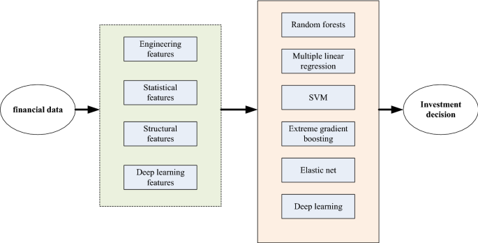
The decision technologies based on deep learning

2.2 Dimension reduction of data based on PCA
Considering the characteristics of e-commerce enterprises and the availability of indicators, this paper chooses the return on net assets, the return on total assets, the quick ratio, the turnover of accounts receivable, the ratio of assets and liabilities, the turnover of inventory, the turnover rate of total assets, the growth rate of business receivers, the cash ratio of business receivers, the R&D input rate, the proportion of R&D technicians, and the authorized issuance owned by thousands of employees of enterprises. The number of patents, capitalization rate of internal R&D, employee productivity, social contribution rate, currency liquidity, and enterprise inventory cycle, product supply–demand relationship, a total of 18 indicators [20].
As a multivariate statistical algorithm, principal component analysis (PCA) can transform most information of high-dimensional raw data variables into low-dimensional linear combinations of these variables through linear mappings, which are called principal components after dimensionality reduction. Replacing the original high-dimensional original variables with these low-dimensional and unrelated comprehensive variables not only reduces the dimensionality of the original data and reduces data redundancy, but also eliminates the correlation between the original variables, simplifies the input structure and reduces the difficulty of modelling and prediction.
The basic principle of principal component analysis is to transform multidimensional linear-related raw data \({\mathbf{X}}_{n \times m}\) into low-dimensional and linear-independent new data \({\mathbf{T}}_{n \times m}\), which \({\mathbf{T}}_{n \times k}\) contains most of the information of the original data \({\mathbf{X}}_{n \times m}\). Let \({\mathbf{X}}\) be the original data, n be the sample number, m be the dimension of the variable, and its mathematical expression is shown in formula (1):
where \(x_{ij}\) is the observed value of the j variable of the first sample, and \({\mathbf{x}}_{m}\) is the sample group of the m variable. But many variables are different in unit and dimension, and there is a big difference in numerical value, so the data need to be standardized.
Matrix \({\mathbf{S}}\) is obtained by normalizing \({\mathbf{X}}\), in which the elements of \({\mathbf{S}}\) matrix correspond to those of original matrix \({\mathbf{X}}\) and are mapped between 0 and 1. \({\mathbf{S}}\) can be expressed as the outer product of score matrix and correlation coefficient matrix.
where the matrix \({\mathbf{R}} = ({\mathbf{r}}_{1} ,{\mathbf{r}}_{2} , \cdots ,{\mathbf{r}}_{m} )\) is the correlation coefficient matrix of \({\mathbf{S}}\); and \({\mathbf{T}} = ({\mathbf{t}}_{1} ,{\mathbf{t}}_{2} , \cdots ,{\mathbf{t}}_{m} )\) score matrix. If \(\left\| {{\mathbf{t}}_{1} } \right\| > \left\| {{\mathbf{t}}_{2} } \right\| > \cdots > \left\| {{\mathbf{t}}_{m} } \right\|\), then \({\mathbf{t}}_{1}\) is the first principal element, representing the maximum projection of the original data \({\mathbf{X}}\) in its corresponding direction.
Taking the first \(k\) principal component, we can get \({\mathbf{S}} = {\mathbf{T}}_{k} {\mathbf{R}}_{k}^{{}} + {\mathbf{E}}\), \({\mathbf{E}}\) is the residual matrix, and \({\mathbf{T}}_{n \times k} = ({\mathbf{t}}_{1} ,{\mathbf{t}}_{2} , \cdots ,{\mathbf{t}}_{k} )\) is the new data after dimensionality reduction.
After the previous screening process, it is found that the number of variables retained is still large, so PCA technology is used to reduce the dimension of variables to simplify the number of network input units.
Before PCA dimension reduction, it is necessary to determine whether there is correlation between variables to test the applicability of PCA. So this paper uses KMO statistical test method. The closer the value \(\delta\) of KMO is to 1, the more suitable the data is to use principal component analysis. The test formulas are as follows:
where \(r_{ij}\) represents the simple correlation coefficients of all variables, and \(a_{ij}\) represents the partial correlation coefficients of all variables. After checking and calculating, the KMO value \(\delta\) of the selected variables is equal to 0.9727, so the selected variables are very suitable for dimension reduction by principal component analysis.
The filtered data will be standardized to eliminate the adverse effects caused by different dimensions. Then the feature values \(\lambda_{1} ,\lambda_{2} , \cdots ,\lambda_{i} , \cdots ,\lambda_{18}\) of the correlation coefficient matrix and its corresponding eigenvector \({\mathbf{p}}_{1} ,{\mathbf{p}}_{2} , \cdots ,{\mathbf{p}}_{i} , \cdots ,{\mathbf{p}}_{18}\) are obtained, and the feature values are arranged from large to small. The formula for calculating cumulative percentage variance (CPV) of feature values is as follows:
where the denominator is the cumulative value of all feature values; the molecule is the cumulative value of the principal element. The most common principal component analysis (PCA) is used to reduce the dimension of data, and less principal components are selected to represent data, which can effectively reduce the follow-up workload and save computing resources. In addition, principal component analysis can also be used for data denoising. The principal component (or sub-component) in the second feature values are often random noise in the data. Cumulative percentage variance and correlation coefficient based on PCA algorithms is shown in Fig. 3.

Cumulative percentage variance and correlation coefficient based on PCA algorithms
2.3 The feature extraction based on deep learning
The purpose of deep learning is to simulate the learning process of the brain, construct a deep-seated model, and learn the implicit characteristics of the data by combining the massive training data, that is, to use large data to learn the characteristics, so as to depict the rich intrinsic information of the data [21]. The commonly used models of deep learning are automatic encoder neural network, depth confidence neural network and convolution neural network. The model adopted in this paper is the cascade noise reduction automatic encoder neural network.
The cascade noise reduction automatic encoder neural network is composed of multiple noise reduction automatic encoders. Automatic encoder is a three-layer unsupervised neural network, which is divided into two parts: coding network and decoding network. Its structure is shown in Fig. 4.

Structure diagram of self-coding network
As we can see from the Fig. 4, the input data and output target of the automatic encoder are the same. The input data of the high-dimensional space is converted into the coding vector of the low-dimensional space by the coding network, and the coding vector of the low-dimensional space is reconstructed back to the original input data by the decoding network. Since the input signal can be reconstructed in the output layer, the coding vector becomes a feature representation of the input data. The structure of denoising auto encoders (DAE) is shown in Fig. 5.

Structure diagram of automatic encoder for noise reduction
As is shown in the Fig. 5, the coding network adds noise with certain statistical characteristics to the sample data, and then codes the sample. The decoding network estimates the original form of the sample which is not disturbed by noise according to the data disturbed by noise, so that DAE learns more robust features from the noisy sample and reduces the sensitivity of DAE to small random disturbances.
The principle of DAE is similar to the human sensory system, such as when the human eye looks at an object, if a small part of it is obscured, the human can still recognize the object. Similarly, the noise reduction automatic encoder can effectively reduce the influence of random factors such as the change of mechanical working conditions and environmental noise on the extracted health information and improve the robustness of feature expression by adding noise to the code reconstruction. The feature colour-map is shown in the Fig. 6.

The extracted feature figure from the financial dataset
As we can see from the Fig. 6, multidimensional dataset calculates and stores all the basic data, metrics and aggregation needed for thematic analysis. In the actual analysis process, the analyst does not include all dimensions, dimension levels and aggregation into the analysis activities, but chooses closely related dimension sets, metrics and aggregation into the analysis activities. Through the combination of dimensions, we can find the best way to explore the problem. Multidimensional view is to meet the needs of users. The minimum granularity of multidimensional view is determined by determining the minimum value of each dimension level, and the path to the problem analysis domain is determined by combining different dimensions, so as to show the metrics and aggregates under different exploration paths and analysis granularity in data sets. The following features are always obtained. The features are expressed in colour-bars.
3 The decision support technology based on deep learning
By investigating the financial and market-related information of listed companies involved in e-commerce industry, starting from the experience and current situation of stock theory research, and using computer modelling, the paper evaluates the quality of e-commerce investment effectively, which is an important basis for Industry and enterprise investors to measure their investment risk and evaluate their investment value. Through the evaluation and analysis of the quality of e-commerce investment, investors can make a more rational prediction of investment returns under the comparative analysis of various investment factors, thus providing a reasonable reference basis for the decision-making of enterprise investors, so as to reduce the blindness in the process of investment decision-making, and can also give quantitative explanations to the different investment perspectives that they pay attention to, so as to realize investment. The purpose of this paper is extending diversity of capital, reducing risk. The whole decision support technology based on deep learning is shown in the Fig. 7.

The decision support technology based on deep learning
As is shown in the Fig. 7, our proposed decision support technology based on deep learning is designed. The decision-making and decision selection are based on the analysis results and experimental results. The data models are the support of the computational mode, which is based on the data-driven way.
3.1 The decision support modelling based on deep learning
The investment stock market is changing rapidly. There are many factors involved in the quality of investment, such as internal, enterprise, macro-factor and so on. They can be divided into political, economic, natural, regional and industrial factors, and the company itself. Among them, there are indirect and direct factors, such as politics and economy, which affect the quality of investment indirectly through influencing the market, the company’s operating conditions and management. Rational level is the factor market that can directly affect investment.
In this paper, GRU (Gated Recurrent Unit) algorithm is used as the training algorithm of the model. Although both BP algorithm and RNN model can be used to train the evaluation prediction model, compared with GRU, their respective shortcomings make them not the optimal algorithm [22, 23]. In traditional BP algorithm, the original data input network can only be input one by one, and the timing relationship between data can not be displayed in training, and the reverse propagation of errors can not be achieved. The process can only be carried out step by step, and the adjustment of parameters is only affected by a single data, and there is no gradient descent process, which can not minimize the convergence of the network. The original data of RNN model can be input at the same time, and the concept of time series is introduced, but the problem of gradient disappearance can not be solved. Therefore, considering the unique advantages of GRU structure, this paper chooses GRU to build the model, as shown in the Fig. 8.

The model structure based on deep learning neural network
In order to improve the accuracy and accuracy of decision-making, inspired by reference, deep recurrent neural network has shown the strong feature extraction and prediction capability for historical time series problems, ranging from language modelling to time series prediction.
where \(D(k|\theta )\) denotes the prediction decision at sample time \(k\); \({x(k - T)}\) and \({x(k - NT)}\) means the state value at sample time \({k - T}\) and \({k - NT}\). \({x(k)}\) contains all the extracted features. \(f( \cdot )\) is a special function that will be learned by the deep recurrent neural network and \(W_{i}\) is a set of parameters in the deep neural network, such as the weight parameters and activation functions. The structure of model based on deep learning is shown in Fig. 7.
The internal structure of the GRU is shown in the Fig. 9; the GRU unit includes Reset gate and Update gate for dealing with information flow. The output of a neuron in GRU networks is calculated as follows:
where \({\mathbf{h}}_{t - 1}\) and \({\mathbf{h}}_{t}\) are the output of hidden layer at time \(t - 1\) and \(t\), \({\mathbf{z}}_{t}\), \({\mathbf{r}}_{t}\) and \({\mathbf{o}}_{t}\) denote the output of update gate, reset gate and neutron at time \(t\). \({\mathbf{W}}^{(z)}\), \({\mathbf{U}}^{(z)}\), \({\mathbf{W}}^{(r)}\), \({\mathbf{U}}^{(r)}\), \({\mathbf{W}}\), and \({\mathbf{U}}\) represent the weight parameters that we be learned during the training process.

The model structure based on deep learning neural network
The internal structure of the GRU unit are shown in the Fig. 9, GRU is a very effective variant of LSTM network. It is simpler and more effective than LSTM network, so it is also a very manifold network. Since GRU is a variant of LSTM, it can also solve the problem of long dependence in RNN network. Three gate functions are introduced in LSTM: input gate, forgetting gate and output gate to control input value, memory value and output value. In the GRU model, there are only two gates: the update gate and the reset gate.
3.2 The discussion of model parameters
In the decision support model based on deep learning, four parameters are needed to be selected.
- 1.
The length of the time window: Sliding window is the ability to frame the time series according to the specified unit length, thus calculating the statistical indicators in the frame. It is equivalent to a certain length of slider sliding on the scale. Each sliding unit can feed back the data in the slider. Simulation results show that considering the 10-s time window of input is always the best choice. Further simulation results indicate that there is no need to consider a longer historical time window than 30 s. The simulation results will be given in next section.
- 2.
Activation function type: Each neuron node in the neural network accepts the output value of the upper neuron as the input value of the neuron, and transmits the input value to the next neuron. The input neuron node will directly transfer the input attribute value to the next neuron (hidden layer or output layer). In multi-layer neural networks, there is a functional relationship between the output of the upper node and the input of the lower node. This function is called activation function (also known as excitation function). For the hidden layer of the neural network, the ‘tanh’ function is chosen as the activation function of the hidden layer (the default activation function in GRU) to decrease the Transfer error during the layers.
$$\tanh x = \frac{{e^{x} - e^{ - x} }}{{e^{x} + e^{ - x} }}$$(10) - 3.
The optimal network structure: The hierarchy of the neural network is generally based on the previous experience. A large number of studies and experiments show that the network with smaller hierarchy has strong generalization ability, easy to understand and extract features, and is conducive to implementation. However, the more hierarchies, the smaller the error of the network will be, which can improve the accuracy and complexity, and increase the training time and speed of the model. As a result of over-fitting, the hierarchy can be set according to the effect of the model. Generally speaking, a three-tier network can be selected for moderate data size and high precision models. Andrey has proved that the three-tier network can fit any non-linear function, and it is also the most widely used network in Multi-tier networks.
- 4.
The weight parameters of the network: Error accuracy should be set according to the specific situation of the model, which requires higher accuracy or stronger generalization ability. The former can set the accuracy smaller, while the latter can be appropriately larger. In the model training, the accuracy can be adjusted according to the results. In addition, the number of sample data and the number of model neurons are correct. Poor precision settings have an impact. The more training data is, the greater the initial error is, and the lower the training accuracy of the model is. Because the larger the scale of the original data, the more variables in the model, the more variables lead to large errors. The error precision is 0.01; Maximal epochs are set as 100.
3.3 The evaluation system of decision support model
The premise of establishing the index evaluation system is that each index is only related to the investment quality, and there is no correlation between the indicators. At present, the mainstream investment quality evaluation indicators in the market or academia are price-earnings ratio, return on net assets, etc. Because of the volatility and risk of the market, they can only serve as a reference. This paper classifies the sample data according to P/E ratio, and does not include all the existing indicators in the evaluation system. The purpose is to find hidden links and grasp the development status of enterprises more accurately by modelling and analyzing the most basic information of e-commerce companies. The selection of indicators reflects the requirements of feasibility, scientific, compliance and quantification. Only by meeting these requirements can the investment direction of enterprises be accurately analyzed. The evaluation system mainly includes: SSE (sum of variance), mean square error (MSE), root mean square error (RMSE), MAE.
In the simulation, the mean absolutely error (MAE) is chosen as the performance index:
where \(D_{e}^{i} (iT|\theta )\) and \(D_{e}^{i} (iT)\) represent the predicted engine torque and real engine torque at sample time \(iT\), respectively. \(i\) is the length of the \(i\)-th time step. \(M\) is the total number of the sample time that are used to train or validation. \(\varOmega\) is the solution space of θ.
Root mean square error (RMSE) is also chosen as the performance index during the simulation:
The coefficient of variation of the RMSE, CV(RMSD), or more commonly CV(RMSE), is defined as the RMSD normalized to the mean of the observed values:
It is the same concept as the coefficient of variation except that RMSD replaces the standard deviation.
4 The simulation and results discussion
4.1 The optimal network selection of model
In this paper, GRU network is used to construct the investment quality evaluation and prediction model. The setting of the number of nodes in the hidden layer is the focus and difficulty of the whole network structure design. There is no uniform standard analytical expression to express the number of nodes. The number of nodes has an important impact on the effect of the whole model. On the one hand, it affects the computing ability of the network; on the other hand, it also affects the approximation ability of the objective function. The more the number of middle-level nodes, the stronger the representational ability, which shows that the data storage capacity of the network is strong, the data processing capacity of each node is small, and the accuracy is high; but once the number of neurons exceeds a certain degree, it will not only increase the learning time, but also affect the realization of the computer, similar to the network hierarchy setting problem.
In this section, as suggested [16], at most 30 percent of training dataset is used for validation we attempt different combinations which is under different size of testing dataset (10%, 15%, 20%, 25%, 30% for testing dataset) and network structures (shown in the Table II in revised paper) to select the appropriate testing dataset and appropriate network structure. As we can see form Fig. 10, results indicate that combinations between the 25% size of the testing dataset and network structure 5 tend to obtain the best performance. On the basis of optimal network structure 6 and 25% of testing dataset, the time window is selected as \({\text{N = }}10\).

The model structure based on deep learning neural network
4.2 The optimal time window selection of model
Hyper-parameter optimization or model selection is the problem of selecting a set of optimal hyperparameters for learning algorithms. Usually the purpose is to measure the performance of optimization algorithms on independent data sets. Cross validation is usually used to estimate this generalization performance. Hyper-parameter optimization is contrasted with practical learning problems, which are usually transformed into optimization problems, but the loss function on the training set is optimized. In fact, learning algorithm learning can well model/reconstruct input parameters, while hyper-parameter optimization ensures that the model does not filter its data through adjustments as it does through regularization.
As is analyzed in last section, the optimal length of time window \(N\) is an important hyper-parameter in the deep recurrent network, the suitable length of time window could make the decision support system obtain the higher accuracy. In this paper, the MAE is taken as performance index to select the appropriate length of the time window.
Figure 11 shows the example of performance index of GRU-based decision support model. As is shown, the test results of the model show that the model with \(N = 9\) yields the optimal performance. Simulation results indicate that the longer length of time window doesn’t need to be considered, since the performance index of model becomes no longer reduced. The optimal length of time window is selected as \(N = 9\). The MAE of the GRU-based network is 73.45.

The optimal length of time window in deep learning model
4.3 The comparison results with other decision algorithms
In order to validate the effectiveness and superiority of the GRU-based decision support model, we attempt the model on the TensorFlow. TensorFlow is an open source framework developed by Google in 2015. By improving DistBelief, the first generation of deep learning system, TensorFlow is faster, more suitable for more platforms and more stable than DistBelief. Sex is stronger, etc. It uses the data flow graph to describe the calculation process, the calculation task is represented by the graph, the data processing is represented by the nodes of the graph, and the data flow is represented by the edge. The lines in the flow chart represent the input and output between the nodes and the whole flow chart represents the input, calculation and output processes of high-dimensional arrays. The comparison results with other algorithms are shown in the Fig. 12.

The comparison results with other algorithms
As we can see form the Fig. 12, GRU-based decision support model can track the real value; the effectiveness of the model is validated. And the tracking performance of the GRU-based decision support model is better than other algorithms. This is because: (1) reducing the interference of manual feature extraction and increasing accuracy; (2) using historical data to make decisions in the model of deep network can effectively improve accuracy; (3) end-to-end network structure can automatically store features and use this feature to make decisions. In this way, our network can obtain better results.
The prediction value has a certain delay compared with the real value. We regard that the reason for this delay phenomenon lies in the operation mechanism of deep recurrent neural network. This is, the prediction value is generated according to the historical information in time window, and instantaneous drivers’ intentions can not ‘feed’ into the neural network, the recurrent neural network can not respond to the driver’s intentions consequently in time. The delay phenomenon becomes obvious when the sharp real value variation occurs.
The detailed comparison results compared with other algorithms are shown in the Table 1. As is shown, the RMSE and MAE indicators are less than other algorithms, and the CV-RMSE indicator is also less than other algorithms. The superiority of our proposed GRU-based decision support model is verified in the paper.
5 Conclusion
In order to improve the accuracy of e-commerce decision-making, this paper proposes an investment decision-making support model in e-commerce based on deep learning calculation to support the company. Investment decision-making system is not only an important means of enterprise investment and financing, but also an important way for investors to make profits. It also plays an important role in macroeconomic regulation, resource allocation and other aspects. This paper takes investment data related to Internet and e-commerce business as the research object, and theory and method of investment decision-making are studied. And then we put forward a prediction model of company decision-making quality evaluation based on deep learning algorithm, aiming at providing decision support for investors. Then a neural network investment quality evaluation model is constructed, including model structure, parameters and algorithm design. The experimental data are input into training, and the data processing process and prediction results are displayed. Experiments show that the evaluation and prediction model is mainly used to judge the quality of investment of Internet or commercial enterprises. Based on this deep learning model, various index data of enterprises are analyzed, which can assist investors in decision-making. Furthermore, this paper provides a new direction for decision-making of e- commerce.
References
Schmidhuber, J. (2015). Deep learning in neural networks: An overview. Neural Networks,61, 85–117.
Ghadai, S., Balu, A., Sarkar, S., et al. (2018). Learning localized features in 3D CAD models for manufacturability analysis of drilled holes. Computer Aided Geometric Design,62, 263–275.
Aouadni, I., & Rebai, A. (2017). Decision support system based on genetic algorithm and multi-criteria satisfaction analysis (MUSA) method for measuring job satisfaction. Annals of Operations Research,256(1), 3–20.
Ghasemi, F., Mehridehnavi, A., Pérez-Garrido, A., et al. (2018). Neural network and deep-learning algorithms used in QSAR studies: Merits and drawbacks. Drug Discovery Today,23(10), 1784–1790.
Yang, Y., Feng, X., Chi, W., et al. (2018). Deep learning aided decision support for pulmonary nodules diagnosing: A review. Journal of Thoracic Disease,10(S7), S867–S875.
Chong, E., Han, C., & Park, F. C. (2017). Deep learning networks for stock market analysis and prediction. Expert Systems with Applications,83, 187–205.
Barros, P., Parisi, G. I., Weber, C., & Wermter, S. (2017). Emotion-modulated attention improves expression recognition: A deep learning model. Neurocomputing,253, 104–114.
Xiao, G., Jaarsveld, W. V., Ming, D., et al. (2018). Models, algorithms and performance analysis for adaptive operatingroom scheduling. International Journal of Production Research,56(4), 1389–1413.
Ślęzak, D., Grzegorowski, M., Janusz, A., et al. (2018). A framework for learning and embedding multi-sensor forecasting models into a decision support system: A case study of methane concentration in coal mines. Information Sciences,451–452, 112–133.
Kraus, M., & Feuerriegel, S. (2017). Decision support from financial disclosures with deep neural networks and transfer learning. Decision Support Systems,104, 38–48.
Nweke, H. F., Ying, W. T., Al-Garadi, M. A., et al. (2018). Deep learning algorithms for human activity recognition using mobile and wearable sensor networks: State of the art and research challenges. Expert Systems with Applications,105, 233–261.
Chen, Miaochao, & Liu, Qilin. (2016). Blow-up criteria of smooth solutions to a 3D model of electro-kinetic fluids in a bounded domain. Electronic Journal of Differential Equations,2016(128), 1–8.
Shameer, K., Badgeley, M. A., Miotto, R., et al. (2017). Translational bioinformatics in the era of real-time biomedical, health care and wellness data streams. Briefings in Bioinformatics,18(1), 105–124.
Sanfey, A. G., Rilling, J. K., Aronson, J. A., Nystrom, L. E., & Cohen, J. D. (2003). The neural basis of economic decision-making in the ultimatum game. Science,300(5626), 1755–1758.
Venkateswara, H., Chakraborty, S., & Panchanathan, S. (2017). Deep-learning systems for domain adaptation in computer vision: Learning transferable feature representations. IEEE Signal Processing Magazine,34(6), 117–129.
Kong, H., Fang, Y., Fan, L., et al. (2019). A novel torque distribution strategy based on deep recurrent neural network for parallel hybrid electric vehicle. IEEE Access,7, 65174–65185.
Zhao, F., Yi, Z., Wang, G., et al. (2018). A brain-inspired decision making model based on top-down biasing of prefrontal cortex to basal ganglia and its application in autonomous UAV explorations. Cognitive Computation,10(2), 296–306.
Komisarczuk, P., Komisarczuk, P., Komisarczuk, P., et al. (2017). A survey on reinforcement learning models and algorithms for traffic signal control. ACM Computing Surveys,50(3), 1–38.
Chen, Miaochao, Shengqi, Lu, & Liu, Qilin. (2018). Global regularity for a 2D model of electro-kinetic fluid in a bounded domain. Acta Mathematicae Applicatae Sinica-English Series,34(2), 398–403.
Kharazmi, P., Zheng, J., Lui, H., et al. (2018). A computer-aided decision support system for detection and localization of cutaneous vasculature in dermoscopy images via deep feature learning. Journal of Medical Systems,42(2), 33.
Sultana, A., Fernando, X., & Zhao, L. (2017). An overview of medium access control strategies for opportunistic spectrum access in cognitive radio networks. Peer-to-Peer Networking and Applications,10(5), 1113–1141.
Böttiger, Y., Laine, K., Korhonen, T., et al. (2018). Development and pilot testing of PHARAO—a decision support system for pharmacological risk assessment in the elderly. European Journal of Clinical Pharmacology,74(3), 365–371.
Ifenthaler, D., & Widanapathirana, C. (2014). Development and validation of a learning analytics framework: Two case studies using support vector machines. Technology, Knowledge and Learning,19(1–2), 221–240.
Author information
Authors and Affiliations
Corresponding author
Ethics declarations
Conflict of interest
The authors declare that there are no conflicts of interest.
Additional information
Publisher's Note
Springer Nature remains neutral with regard to jurisdictional claims in published maps and institutional affiliations.
Rights and permissions
About this article

Cite this article
Lei, Z. Research and analysis of deep learning algorithms for investment decision support model in electronic commerce. Electron Commer Res 20, 275–295 (2020). https://doi.org/10.1007/s10660-019-09389-w
Published:
Issue Date:
DOI: https://doi.org/10.1007/s10660-019-09389-w