On the Statistical Dependence for the Components of Random Elasticity Tensors Exhibiting Material Symmetry Properties

Abstract

This work is concerned with the characterization of the statistical dependence between the components of random elasticity tensors that exhibit some given material symmetries. Such an issue has historically been addressed with no particular reliance on probabilistic reasoning, ending up in almost all cases with independent (or even some deterministic) variables. Therefore, we propose a contribution to the field by having recourse to the Information Theory. Specifically, we first introduce a probabilistic methodology that allows for such a dependence to be rigorously characterized and which relies on the Maximum Entropy (MaxEnt) principle. We then discuss the induced dependence for the highest levels of elastic symmetries, ranging from isotropy to orthotropy. It is shown for instance that for the isotropic class, the bulk and shear moduli turn out to be independent Gamma-distributed random variables, whereas the associated stochastic Young modulus and Poisson ratio are statistically dependent random variables.

1 Introduction

This work is devoted to the characterization of the statistical dependence for the components of random elasticity tensors. Such randomness can be encountered for several reasons, among which:

• The presence of uncertainties while modeling the experimental setup in either forward simulations or inverse identification.

• The lack of scale separation for heterogeneous random materials, hence resulting in the consideration of mesoscopic, apparent properties.

In the former case, one may consider uncertainties on a macroscopic elasticity tensor, whereas the second situation may involve the construction of probabilistic models for mesoscale random fields with values in the set of elasticity tensors (see [17] and the references therein). In practice, such a construction can be carried out by introducing a non-linear transformation acting on a set of homogeneous Gaussian random fields (see [26] for details about the overall methodology, as well as [4–6] for further applications to random fields of elasticity tensors). The aforementioned mapping can be defined by specifying the family of first-order marginal distributions for the random field and thus requires the probability distribution of random elasticity tensors to be defined. In this paper, we focus on the stochastic modeling of elasticity tensors which exhibit a.s. (almost surely) some material symmetry properties. In such cases, one typically wonders whether or not the considered elastic moduli may be modeled as dependent random variables: are the random Young modulus and Poisson ratio, associated with random isotropic tensors, statistically dependent? If so, how should such a dependence be integrated without introducing any modeling bias (i.e. model uncertainties)?

In this context, uncertainty propagation is often based on strong assumptions regarding the probability distributions, which are mostly chosen for the sake of theoretical and numerical convenience rather than deduced from a probabilistic reasoning. Consequently, such models arguably suffer from end-user’s subjectivity and may be questionable from both a mechanical and mathematical standpoint.

In this work, we address such an issue from the point of view of Information Theory and construct a prior stochastic model for the elasticity tensor. More specifically, we introduce a probabilistic methodology, based on a particular decomposition of the elasticity tensors, which allows for the aforementioned dependence to be rigorously characterized and discussed for the highest levels of elastic symmetries, ranging from isotropy to orthotropy (see [2], among others, for a discussion about the definition of such symmetries). Fundamental mathematical properties of random elasticity tensors, such as variance finiteness, are further taken into account in order to ensure the physical consistency of the model.

This paper is organized as follows. Section 2 is devoted to the overall probabilistic methodology. In particular, the tensor decomposition is introduced and the framework of Information Theory, together with the Maximum Entropy principle, is briefly stated. The induced general form for the prior probability distributions of the random components is then explicitly given. In Sect. 3, we derive the probability distributions for the random components of elasticity tensors exhibiting various symmetry properties and highlight the resulting statistical dependence. It is shown that the latter depends on the retained parametrization (i.e., on the choice of the tensor decomposition), as well as on the considered class of symmetry.

2 Probabilistic Modeling of Elasticity Tensors

2.1 Notations

Throughout this paper, we use double (e.g., 〚C〛) and single (e.g., [C]) brackets to denote fourth-order and second-order elasticity tensors respectively, the latter being defined with respect to the Kelvin matrix representation (see [14] for a discussion). We denote by $\mathbb{M}_{n}^{+}(\mathbb{R})$ the set of all the (n×n) real symmetric positive-definite matrices.

2.2 Tensor Decomposition

Let $\mathbb{E}\mathrm{la}$ be the set of all the fourth-order elasticity tensors verifying the usual properties of symmetries and positiveness. Hereafter, we denote by $\mathbb {E}\mathrm {la}^{\mathrm {sym}}\subseteq\mathbb{E}\mathrm{la}$ the subset of all the fourth-order elasticity tensors belonging to the material symmetry class ‘sym’. It is well-known that any element can be decomposed as

(1)

where is a tensor basis of $\mathbb {E}\mathrm {la}^{\mathrm {sym}}$ and $\{c_{i}\}_{i = 1}^{N}$ is a set of coefficients satisfying some algebraic properties related to the positiveness of 〚C ^sym〛.

Extending the aforementioned decomposition to the case of random elasticity tensors, we then denote by 〚C ^sym〛 the random variable with values in $\mathbb {E}\mathrm {la}^{\mathrm {sym}}$, the probability distribution of which is sought, and similarly write

(2)

where $\{C_{i}\}_{i = 1}^{N}$ is now a set of random variables whose probability distributions and mutual statistical dependence must be defined.

The definition of tensor basis for various classes of symmetry has been largely investigated within the past four decades and we refer the interested reader to the literature available on this subject (see Sect. II.B of [30], as well as [12]). In this paper, we make use of Walpole’s derivations and follow the notations and formalism proposed in [29], allowing for simplified algebraic operations on tensors in $\mathbb{E}\mathrm{la}$. Such representations have been used to define projection operators onto subsets of $\mathbb{E}\mathrm{la}$ with given symmetries in [16], for instance. For the sake of self-readability, the expressions for tensor basis will be recalled for all the symmetry classes investigated in Sect. 3. A stochastic elasticity matrix [C ^sym] can then be modeled as a $\mathbb{M}_{n}^{\mathrm{sym}}(\mathbb{R})$-valued random variable (with $\mathbb{M}_{n}^{\mathrm{sym}}(\mathbb{R}) \subseteq\mathbb {M}_{n}^{+}(\mathbb{R})$) and can be written as

$$ \bigl[\mathbf{C}^{\mathrm{sym}} \bigr] = \sum_{i =1}^{N} C_i \bigl[{E_{\mathrm{sym}}}^{(i)} \bigr], $$

(3)

wherein [E _sym ⁽ⁱ⁾] is the deterministic matrix representation of the fourth-order basis tensor 〚E _sym ⁽ⁱ⁾〛 (which is not orthonormal, except for the isotropic case [29]) and $\mathbb{M}_{n}^{\mathrm{sym}}(\mathbb{R}) = \mathrm {span}([{E_{\mathrm{sym}}}^{(1)}], \ldots, [{E_{\mathrm{sym}}}^{(N)}])$. Thus, the construction of a probabilistic model for the random elasticity tensor 〚C ^sym〛 is strictly equivalent to the construction of a model for the random coordinates C ₁,…,C _N , and such an issue is now to be addressed in Sect. 2.3.

2.3 Methodology for the Probabilistic Model Derivation

Let C=(C ₁,…,C _N ) be the ℝ^N-valued second-order random variable corresponding to the modeling of the random coordinates of [C ^sym] onto $\{ [{E_{\mathrm{sym}}}^{(i)}]\}_{i = 1}^{N}$. We denote by P _C its unknown probability distribution, which is defined by a probability density function (p.d.f.) p _C with respect to the Lebesgue measure dc=dc ₁…dc _N , P _C (dc)=p _C (c)dc. We denote by $\mathcal{S}$ the support of p _C . It is worthwhile to note that because of the a.s. positive-definiteness of [C ^sym], $\mathcal{S}$ is a part, possibly unbounded, of ℝ^N, the definition of which basically depends on the considered material symmetry class.

The prior probability model for random vector C is constructed by having recourse to the Maximum Entropy (MaxEnt) principle, which is a general stochastic optimization procedure derived within the framework of Information Theory [21, 22] and which allows for the explicit construction of probability distributions under a set of constraints defining some available information [7–9]. The definition of the latter turns out to be the cornerstone of the approach, for it aims at ensuring the objectivity of the model. At this stage of writing, let us simply assume that all the constraints related to such information can be put in the form of a mathematical expectation:

$$ \mathrm{E} \bigl\{\mathbf{f}(\mathbf{C}) \bigr\} = \mathbf{h}, $$

(4)

where c↦f(c) is a given measurable mapping from ℝ^N into ℝ^q and h is a given vector in ℝ^q. It is assumed that one of the constraints in Eq. (4) corresponds to the normalization condition of the p.d.f. (see Eq. (8)). Let $\mathcal {C}_{\mathrm{ad}}$ be the set of all the integrable functions from $\mathcal{S} \subset\mathbb {R}^{N}$ into ℝ⁺ such that Eq. (4) is satisfied and let $\mathcal{E}(p)$ be the so-called Shannon measure of entropy of p.d.f. p:

$$ \mathcal{E}(p) = - \int_{\mathcal{S}} p(\mathbf{c}) \ln\bigl(p(\mathbf{c})\bigr) \, \mathrm{d}\mathbf{c}. $$

(5)

The MaxEnt principle then reads:

$$ p_{\mathbf{C}} = \mathop {\mathrm {arg\,max}}_{p \in \mathcal{C}_{\mathrm{ad}}} \mathcal{E}(p). $$

(6)

In other words, the probability density function estimated by the MaxEnt principle is the function which maximizes the uncertainties under the set of constraints stated by Eq. (4). Consequently, this approach is intended to yield the most objective probabilistic model and has been successfully used in various fields of application (see [10, 11, 23] and the references therein, for instance). We assume that the optimization problem stated by Eq. (6) is well-posed in the sense that the above constraints are algebraically independent (see Appendix B), so that the optimization problem given by Eq. (6) admits at most one solution. Under this assumption (which is satisfied hereafter), the general form of the solution for the stochastic optimization problem (6) can be obtained by introducing a set of Lagrange multipliers and by proceeding to the calculus of variations, whereas the uniqueness of the solution Lagrange multiplier (the existence of which must be studied) can be deduced from a standard argument of optimization for a strictly convex function which is associated with $\mathcal{E}$ and the constraints (see Appendix B for the construction of such a strictly convex function). Below, we assume that such a solution Lagrange multiplier exists (see the discussion in Appendix B).

In the case of elasticity tensors, three fundamental properties are worth taking into account, that are:

$\mathcal{P}_{1}$::

the mean value of the tensor, denoted by $[\underline{C}^{\mathrm{sym}}]$, is given (and could correspond to the nominal, expected value);

$\mathcal{P}_{2}$::

the elasticity tensor, as well as its inverse, has a finite second-order moment (for physical consistency);

$\mathcal{P}_{3}$::

the p.d.f. p _C satisfies the usual normalization condition.

Although additional information could be considered, the information defined above basically corresponds to the most basic properties satisfied by [C] (since $\mathcal{P}_{2}$ and $\mathcal{P}_{3}$ are a.s. mathematical properties and $\mathcal{P}_{1}$ corresponds to the very first property that may be estimated from experimental measurements) and thus, the consequence of such constraints on the statistical dependence of the random components is of primary importance. Mathematically, the properties $\mathcal{P}_{1}$ and $\mathcal{P}_{3}$ can be written as

$$ \mathrm{E}\{\mathbf{C}\} = \underline{ \mathbf{c}}, \quad\underline{\mathbf{c}} = (\underline{c}_1, \ldots, \underline{c}_N) $$

(7)

and

$$ \int_\mathcal{S} p_{\mathbf{C}}(\mathbf{c}) \, \mathrm{d}\mathbf{c} = 1, $$

(8)

while the second property $\mathcal{P}_{2}$ can be stated as (see [24, 25]):

$$ \mathrm{E} \Biggl\{\log\Biggl( \det\Biggl(\sum_{i =1}^{N} C_i \bigl[{E_{\mathrm{sym}}}^{(i)}\bigr] \Biggr) \Biggr) \Biggr\} = \nu_{\mathbf{C}}, \quad|\nu_{\mathbf{C}}| < +\infty, $$

(9)

where ν _C is a given parameter (q=N+2). Let $\boldsymbol{\lambda}^{(1)} \in\mathcal{A}_{\boldsymbol{\lambda }^{(1)}} \subset \mathbb{R}^{N}$, $\lambda^{(2)} \in\mathcal{A}_{\lambda^{(2)}} \subset\mathbb{R}$ and λ ⁽⁰⁾∈ℝ⁺ be the Lagrange multipliers associated with constraints (7), (9) and (8) respectively. Let $\boldsymbol{\lambda}=(\boldsymbol{\lambda}^{(1)}, \lambda^{(2)}) \in \mathcal{A}_{\mathbf{\lambda}}$, with $\mathcal{A}_{\boldsymbol {\lambda}} = \mathcal{A}_{\boldsymbol{\lambda}^{(1)}} \times\mathcal {A}_{\lambda^{(2)}}$, and let $\lambda^{(0)}_{\mathrm{sol}}$ and $\boldsymbol{\lambda}_{\mathrm{sol}}=(\boldsymbol{\lambda }_{\mathrm{sol}}^{(1)}, \lambda_{\mathrm{sol}}^{(2)})$ be the solution Lagrange multipliers such that Eqs. (8), (7) and (9) are satisfied. It can be shown that the p.d.f. p _C takes the general form (see also [7, 8] for random vectors and [1] for similar results in case of random matrices [15], for instance)

(10)

in which:

• is the characteristic function of $\mathcal{S}$, i.e. if $\mathbf{c} \in\mathcal{S}$, 0 otherwise;

• $k_{\mathrm{sol}} = \exp\{-\lambda^{(0)}_{\mathrm{sol}}\}$ is the normalization constant;

• c↦g(c) is the mapping defined on $\mathcal{S}$, with values in ℝ^N+1, such that g(c)=(c,φ(c));

• the mapping $\varphi: \mathcal{S} \longrightarrow\mathbb{R}$ is given by

  $$ \varphi(\mathbf{c}) = \log\Biggl( \det \Biggl( \sum _{i =1}^{N} c_i \bigl[{E_{\mathrm{sym}}}^{(i)}\bigr] \Biggr) \Biggr). $$

  (11)

The existence of the Lagrange multiplier λ _sol (as well as its value, should it exist) can be numerically studied, either by substituting λ for λ _sol in Eq. (10) and by minimizing (with respect to some given metric) the discrepancy between the left- and right-hand sides of Eqs. (7) and (9), or by minimizing the convex function introduced in Appendix B. The mathematical expectations can be computed by using a numerical Monte Carlo integration, for instance. In addition, this approach requires the use of an efficient random generator and the use of a Markov Chain Monte Carlo technique [19] is a natural choice to this aim [27]. It should be noticed that the admissible space $\mathcal{A}_{\mathbf{\lambda}}$ for the Lagrange multipliers must be defined in order to preserve the integrability of the p.d.f. (10) at both the origin and infinity. Once the p.d.f. has been determined (by solving Eq. (6)), it can then be seen in practice that the level of statistical fluctuations of the random elasticity matrix, characterized by a scalar parameter δ _C defined as

$$ \delta_{\mathbf{C}}^2 = \mathrm{E}\bigl\{\bigl\|\bigl[ \mathbf{C}^{\mathrm{sym}}\bigr] - \bigl[\underline{C}^{\mathrm {sym}}\bigr] \bigr\|_{\mathrm{F}}^2\bigr\}/\bigl\|\bigl[\underline{C}^{\mathrm {sym}}\bigr] \bigr\|_{\mathrm{F}}^2, $$

(12)

depends on the prescribed mean value $\underline{\mathbf{c}}$ and on the Lagrange multiplier associated with the constraint given by Eq. (9) (see [24]). The constant ν _C could therefore be reparametrized in terms of the mean value $\underline{\mathbf{c}}$ and dispersion parameter δ _C .

The p.d.f. p _C can be finally rewritten as:

(13)

The statistical dependence of the random components can then be characterized, in view of Eq. (13), by studying the separability of mapping c↦φ(c). It is interesting to note that this dependence intrinsically depends on the retained parametrization, as the latter yields a particular form for the determinant involved in the definition of the mapping φ (see Eq. (11)).

Before discussing such an issue further, it is instructive to note that typical assumptions used in practical applications consist in imposing the mean and second-order moments of all the random coordinates. In this case, a straightforward analogy with the previous derivations allows us to write the p.d.f. p _C as

(14)

where $\lambda_{\mathrm{sol}}^{(2)} \in\mathcal{A}_{\lambda^{(2)}} \subseteq\mathbb{R}^{N}$ is the Lagrange multiplier associated with the constraint on second-order moments and k is the normalization constant. Using such information, one therefore ends up with random coordinates whose mutual statistical dependence can be defined by studying the separability of . Subsequently, it will be shown that the invertibility constraint stated by $\mathcal {P}_{2}$, which is absolutely fundamental in order to ensure physical consistency, also creates some statistical dependence structure that is specific to the symmetry class.

In the next section, we investigate the statistical dependence between the random coefficients induced by the MaxEnt principle (for which the available information is stated by properties $\mathcal{P}_{1}$, $\mathcal{P}_{2}$ and $\mathcal {P}_{3}$), for the sixth highest levels of material symmetry (i.e., from isotropic to orthotropic symmetries). The case of the monoclinic symmetry is less attractive, since it is barely encountered in practice (except for crystallographic considerations), and the case of triclinic materials has been considered in [28].

Remark on correlation structure

Let 〚R〛 be the fourth-order covariance tensor of random matrix [C], defined as:

(15)

with $[\underline{C}] = \mathrm{E}\{[\mathbf{C}]\}$ the mean value of [C]. Notice that the term 〚R〛 _αβαβ then represents the variance of random variable [C] _αβ . The correlation structure described by 〚R〛 is then completely characterized by the probability distributions of random components $\{C_{i}\}_{i = 1}^{i=N}$ and tensor basis $\{[{E_{\mathrm{sym}}}^{(i)}]\}_{i = 1}^{i=N}$, since

(16)

with $C_{i}^{*} = C_{i} - \underline{c}_{i}$. When all the random components are statistically independent from one another, Eq. (16) simplifies to:

(17)

in which $\mathcal{V}_{i}$ denotes the variance of C _i .

3 Results

For notational convenience, let us set $\boldsymbol{\lambda}_{\mathrm {sol}}^{(1)} = (\lambda_{1}, \ldots, \lambda_{N})$, $\lambda_{\mathrm{sol}}^{(2)} = \lambda$. For calculation purposes and without loss of generality, any triad (a,b,c) of mutually orthonormal vectors makes reference to the canonical basis in ℝ³ (i.e., a=(1,0,0) for instance). Whenever the definition of a specific axis is required, we take this vector as (0,0,1).

3.1 Isotropic Symmetry

Let the isotropic random elasticity matrix [C] be decomposed as

$$ [\mathbf{C}] = 3 C_1 \bigl[E^{(1)}\bigr] + 2 C_2 \bigl[E^{(2)}\bigr], $$

(18)

where C ₁ and C ₂ are the random bulk and shear moduli, [E ⁽¹⁾] and [E ⁽²⁾] being the matrix representation of the classical fourth-order symmetric tensors 〚E ⁽¹⁾〛 and 〚E ⁽²⁾〛 defined by

in which 〚I〛 represents the fourth-order symmetric identity tensor (〚I〛 _ijkℓ =(δ _ik δ _jℓ +δ _iℓ δ _jk )/2).

Proposition 1

For the isotropic class, the bulk and shear random moduli C ₁ and C ₂ involved in the tensor decomposition given by Eq. (18) are statistically independent Gamma-distributed random variables, with respective parameters $(1 - \lambda, \underline{c}_{1}/(1-\lambda))$ and $(1 - 5\lambda, \underline {c}_{2}/(1-5\lambda))$, where $\underline{c}_{1}$ and $\underline{c}_{2}$ are the given mean values of C ₁ and C ₂ and λ∈ ]−∞,1/5[ is a model parameter controlling the level of statistical fluctuations.

Proof

From Eq. (18), one can deduce that:

$$ \varphi(\mathbf{c}) = \log\bigl\{ 96 \, c_1 {c_2}^5\bigr\}. $$

(19)

It follows that

$$ p_{\mathbf{C}}(\mathbf{c}) = p_{C_1}(c_1) \times p_{C_2}(c_2), $$

(20)

with

(21)

and

(22)

where k ₁ and k ₂ are positive normalization constants. Thus, the random bulk and shear moduli are Gamma-distributed statistically independent random variables, with parameters (α ₁,β ₁)=(1−λ,1/λ ₁) and (α ₂,β ₂)=(1−5λ,1/λ ₂). The normalization constants k ₁ and k ₂ are then found to be k ₁=λ ₁ ^1−λ/Γ(1−λ) and k ₂=λ ₂ ^1−5λ/Γ(1−5λ), while it can be deduced that $\underline{c}_{1}=(1-\lambda)/\lambda_{1}$ and $\underline {c}_{2}=(1-5\lambda)/\lambda_{2}$. □

The coefficients of variation of the bulk and shear moduli are then given by $1/\sqrt{1-\lambda}$ and $1/\sqrt{1-5\lambda}$ respectively, showing that the two moduli do not exhibit the same level of fluctuations.

Let E and ν be the random Young modulus and Poisson ratio associated with the isotropic random elasticity tensor, defined as E=9C ₁ C ₂/(3C ₁+C ₂) and ν=(3C ₁−2C ₂)/(6C ₁+2C ₂). The joint p.d.f. (e,n)↦p _E,ν (e,n) of random variables E and ν can be readily deduced from Eqs. (20), (21) and (22) and is found to be given by

(23)

with $\mathcal{S} = \,]0, +\infty[\, \times\,]{-}1, 1/2[$. Consequently, the random Young modulus and Poisson ratio turn out to be statistically dependent random variables.

3.2 Cubic Symmetry

Let (a,b,c) be the unit mutually orthogonal vectors defining the crystallographic directions of the cubic system and let the random elasticity matrix [C] exhibiting cubic symmetry be decomposed as

$$ [\mathbf{C}] = C_1 \bigl[E^{(1)}\bigr] + C_2 \bigl[E^{(2)}\bigr] + C_3 \bigl[E^{(3)}\bigr], $$

(24)

where:

• [E ⁽¹⁾] is the matrix form of tensor 〚E ⁽¹⁾〛 defined in Sect. 3.1;

• [E ⁽²⁾] and [E ⁽³⁾] are the matrix representations of fourth-order tensors 〚E ⁽²⁾〛=〚I〛−〚S〛 and 〚E ⁽³⁾〛=〚S〛−〚E ⁽¹⁾〛, with 〚S〛 _ijkℓ =a _i a _j a _k a _ℓ +b _i b _j b _k b _ℓ +c _i c _j c _k c _ℓ .

Proposition 2

For the cubic case, the random components C ₁, C ₂ and C ₃ involved in the tensor decomposition given by Eq. (24) are statistically independent and Gamma-distributed, with respective parameters $(1-\lambda, \underline{c}_{1}/(1-\lambda))$, $(1-3\lambda, \underline {c}_{2}/(1-3\lambda))$ and $(1-2\lambda, \underline{c}_{3}/(1-2\lambda))$, where $\underline{c}_{1}$, $\underline{c}_{2}$ and $\underline{c}_{3}$ are the given mean values of C ₁, C ₂ and C ₃ and λ∈ ]−∞,1/3[ is a model parameter controlling the level of fluctuation.

Proof

From Eq. (24), it can be shown that:

$$ \varphi(\mathbf{c}) = \log\bigl\{ c_1 {c_2}^3 {c_3}^2 \bigr\}. $$

(25)

Therefore, it follows that

$$ p_{\mathbf{C}}(\mathbf{c}) = p_{C_1}(c_1) \times p_{C_2}(c_2) \times p_{C_3}(c_3), $$

(26)

with

(27)

(28)

and

(29)

where k ₁, k ₂ and k ₃ are positive normalization constants. It can be deduced that the random moduli C ₁, C ₂ and C ₃ are Gamma-distributed statistically independent random variables, with respective parameters (α ₁,β ₁)=(1−λ,1/λ ₁), (α ₂,β ₂)=(1−3λ,1/λ ₂) and (α ₃,β ₃)=(1−2λ,1/λ ₃). The expressions for the normalization constants and mean values directly follow, yielding the general form of the p.d.f. □

3.3 Transversely Isotropic Symmetry

Let n be the unit normal orthogonal to the plane of isotropy and let [C] be decomposed as

$$ [\mathbf{C}] = C_1 \bigl[E^{(1)}\bigr] + C_2 \bigl[E^{(2)}\bigr] + C_3 \bigl(\bigl[E^{(3)}\bigr] + \bigl[E^{(4)}\bigr] \bigr) + C_4 \bigl[E^{(5)}\bigr] + C_5 \bigl[E^{(6)}\bigr], $$

(30)

where [E ⁽¹⁾],…,[E ⁽⁶⁾] are the matrix representations of the fourth-order tensors defined as 〚E ⁽¹⁾〛=[p]⊗[p], , , , 〚E ⁽⁵⁾〛=[q]⊙[q]−〚E ⁽²⁾〛 and 〚E ⁽⁶⁾〛=〚I〛−〚E ⁽¹⁾〛−〚E ⁽²⁾〛−〚E ⁽⁵⁾〛. In these expressions, the two second-order symmetric tensors [p] and [q] are defined by [p]=n⊗n and [q]=[I]−[p], with [I] the second-rank symmetric identity tensor and ⊙ the usual symmetrized tensor product, defined by 2([A]⊙[B]) _ijkℓ =[A] _ik [B] _jℓ +[A] _iℓ [B] _jk for any second-order tensors [A] and [B].

Proposition 3

For the transverse isotropic case, the random components C _i , i=1,…,5, involved in the tensor decomposition given by Eq. (30) are such that:

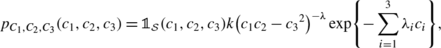
• (i) the components C ₁, C ₂ and C ₃ are statistically dependent random variables whose joint p.d.f. $(c_{1}, c_{2}, c_{3}) \mapsto p_{C_{1}, C_{2}, C_{3}}(c_{1}, c_{2}, c_{3})$ is given by:

  

  (31)

  in which

  $$\mathcal{S} = \bigl\{(x, y, z) \in\mathbb{R}^+ \times\mathbb{R}^+ \times\mathbb{R}\ \mbox{\textit{such\ that}}\ xy - z^2 > 0\bigr\} $$

  and k is a normalization constant

• (ii) the components C ₄ and C ₅ are statistically independent and Gamma-distributed, with respective parameters $(1-2\lambda, \underline{c}_{4}/(1-2\lambda))$ and $(1-2\lambda, \underline{c}_{5}/(1-2\lambda))$, where $\underline{c}_{4}$ and $\underline{c}_{5}$ are the given mean values of C ₄ and C ₅ and λ∈ ]−∞,1/2[ is a model parameter controlling the level of statistical fluctuations

• (iii) the random variables A=(C ₁,C ₂,C ₃), C ₄ and C ₅ are statistically independent.

Proof

It can be shown that

$$ \varphi(\mathbf{c}) = \log\bigl\{ \bigl(c_1 c_2 - {c_3}^2\bigr) {c_4}^2 {c_5}^2 \bigr\}, $$

(32)

so that the p.d.f. p _C takes the form

$$ p_{\mathbf{C}}(\mathbf{c}) = p_{C_1, C_2, C_3}(c_1, c_2, c_3) \times p_{C_4}(c_4) \times p_{C_5}(c_5), $$

(33)

with $p_{C_{1}, C_{2}, C_{3}}$ defined by Eq. (31) and

(34)

(35)

Therefore, the random components C ₁, C ₂ and C ₃ are statistically dependent and are jointly distributed with respect to the p.d.f. given by Eq. (31), whereas C ₄ and C ₅ are Gamma-distributed statistically independent random variables with parameters (α ₄,β ₄)=(1−2λ,1/λ ₄) and (α ₅,β ₅)=(1−2λ,1/λ ₅). The definition of the support $\mathcal{S}$ is readily deduced from the a.s. positive-definiteness of the random elasticity tensor. □

Unlike the cases of isotropic and cubic symmetries, it is seen that some of the components of a random elasticity matrix exhibiting transverse isotropy are statistically dependent, the remaining components being independent from all others. It is also interesting to notice that the two components C ₄ and C ₅ exhibit the same level of statistical fluctuations, with a coefficient of variation equal to $1/\sqrt{1-\lambda}$.

3.4 Tetragonal Symmetry

Let (a,b,c) be unit mutually orthogonal vectors, with c identified as a principal axis of symmetry.

3.4.1 General Case

The most general definition of a tensor basis for the tetragonal symmetry necessitates the consideration of the tensors and 〚E ⁽⁶⁾〛 (renumbered as 〚E ⁽⁹⁾〛), introduced for the transversely isotropic class (taking the principal axis of symmetry c as n; see Sect. 3.3). It further requires the definition of four additional tensors given by:

(36)

The tetragonal random elasticity tensor can be written as

(37)

in which the matrix representations of the aforementioned tensors is used.

Proposition 4

For the tetragonal case (parametrized by seven moduli), the random components C _i , i=1,…,7, involved in the tensor decomposition given by Eq. (37) are such that:

• (i) the components C ₁, C ₂ and C ₃ are statistically dependent random variables whose joint p.d.f. $(c_{1}, c_{2}, c_{3}) \mapsto p_{C_{1}, C_{2}, C_{3}}(c_{1}, c_{2}, c_{3})$ is given by:

  

  (38)

  in which

  $$\mathcal{S} = \bigl\{(x, y, z) \in\mathbb{R}^+ \times\mathbb{R}^+ \times\mathbb{R}\ \mbox{\textit{such that}}\ xy - z^2 > 0\bigr\} $$

  and k is a normalization constant

• (ii) the components C ₄, C ₅ and C ₆ are statistically dependent random variables whose joint p.d.f. $(c_{4}, c_{5}, c_{6}) \mapsto p_{C_{4}, C_{5},C_{6}}(c_{4}, c_{5}, c_{6})$ is given by:

  

  (39)

  where k ^∗ is a normalization constant

• (iii) the component C ₇ is a Gamma-distributed random variable, with parameters $(1-2\lambda, \underline{c}_{7}/(1-2\lambda))$, where $\underline {c}_{7}$ is the given mean value of C ₇ and λ∈ ]−∞,1/2[ is a model parameter controlling the level of statistical fluctuations

• (iv) the three random variables A=(C ₁,C ₂,C ₃), B=(C ₄,C ₅,C ₆) and C ₇ are statistically independent.

Proof

For the tetragonal symmetry and seven-parameters decomposition, one has:

$$ \varphi(\mathbf{c}) = \log\bigl\{ \bigl(c_1 c_2 -{c_3}^2\bigr) \bigl(c_4 c_5 - {c_6}^2\bigr) {c_7}^2 \bigr\}. $$

(40)

Consequently, it follows that:

$$ p_{\mathbf{C}}(\mathbf{c}) = p_{C_1, C_2, C_3} (c_1, c_2, c_3 ) \times p_{C_4, C_5, C_6} (c_4, c_5, c_6 ) \times p_{C_7}(c_7), $$

(41)

with

(42)

(43)

and

(44)

 □

3.4.2 Reduced Parametrization

The tetragonal class is often considered as being parametrized by six coefficients. Indeed, such a representation can be readily obtained from the previous one (see Eq. (37)) by a specific rotation, such that the coefficient C ₆ vanishes [3]. The tensor decomposition then reads:

(45)

Proposition 5

For the tetragonal case with reduced parametrization, the random components C _i , i=1,…,6, involved in the tensor decomposition given by Eq. (45) are such that:

• (i) the components C ₁, C ₂ and C ₃ are statistically dependent random variables whose joint p.d.f. $(c_{1}, c_{2}, c_{3}) \mapsto p_{C_{1}, C_{2}, C_{3}}(c_{1}, c_{2}, c_{3})$ is given by:

  

  (46)

  in which

  $$\mathcal{S} = \bigl\{(x, y, z) \in\mathbb{R}^+ \times\mathbb{R}^+ \times\mathbb{R} \mbox{ \textit{such that} } xy - z^2 > 0\bigr\} $$

  and k is a normalization constant

• (ii) the components C ₄, C ₅ and C ₆ are statistically independent and Gamma-distributed, with respective parameters $(1-\lambda, \underline{c}_{4}/(1-\lambda))$, $(1-\lambda, \underline {c}_{5}/(1-\lambda))$ and $(1-2\lambda, \underline{c}_{6}/ (1-2\lambda))$, where $\underline{c}_{4}$, $\underline{c}_{5}$ and $\underline{c}_{6}$ are the given mean values of C ₄, C ₅ and C ₆, and λ∈ ]−∞,1/2[ is a model parameter controlling the level of statistical fluctuations

• (iii) the random variables A=(C ₁,C ₂,C ₃), C ₄, C ₅ and C ₆ are statistically independent.

Proof

One has:

$$ \varphi(\mathbf{c}) = \log\bigl\{ \bigl(c_1 c_2 - {c_3}^2\bigr) c_4 c_5 {c_6}^2 \bigr\}. $$

(47)

Therefore, the p.d.f. p _C takes the form

$$ p_{\mathbf{C}}(\mathbf {c}) = p_{C_1, C_2, C_3} (c_1, c_2, c_3 ) \times p_{C_4}(c_4) \times p_{C_5}(c_5) \times p_{C_6}(c_6), $$

(48)

with

(49)

(50)

(51)

and

(52)

 □

3.5 Trigonal Symmetry

In order to investigate the statistical dependence of the random components for the trigonal symmetry (which is basically referred to as the hexagonal one in [29]), let us consider three unit vectors denoted by a, b and c, such that c is orthogonal to the plane spanned by a and b, an angle of 2π/3 being left between the latter. Here, the values a=(1,0,0), $\mathbf{b} = (-1/2, \sqrt{3}/2, 0)$ and c=(0,0,1) have been retained.

3.5.1 General Case

Let us introduce the following symmetric second-order tensors

$$ \left\{ \begin{array}{l} [s] = \sqrt{2/3} (\mathbf{a} \otimes\mathbf{a} + \mathbf{a} \otimes\mathbf{b} + \mathbf{b} \otimes\mathbf{a}), \\[1mm] [t] = \sqrt{2/3} (\mathbf{b} \otimes\mathbf{b} + \mathbf{a} \otimes\mathbf{b} + \mathbf{b} \otimes\mathbf{a}), \\[1mm] [u] = (1/\sqrt{2}) (\mathbf{c} \otimes\mathbf{a} + \mathbf{a} \otimes\mathbf{c}), \\[1mm] [v] = -(1/\sqrt{2}) (\mathbf{c} \otimes\mathbf{b} + \mathbf{b} \otimes\mathbf{c}), \end{array} \right. $$

from which the four symmetric tensors

(53)

and the two unsymmetric tensors

(54)

can be defined. The random elasticity tensor is now decomposed as:

(55)

wherein the matrix set $\{[E^{(i)}]\}_{i = 1}^{i = 4}$ coincides with the one introduced for the transverse isotropy case (see Sect. 3.3), setting n=c, and [E ⁽ⁱ⁾] is the matrix form of fourth-order tensor 〚E ⁽ⁱ⁾〛.

Proposition 6

For the trigonal case (parametrized by seven moduli), the random components C _i , i=1,…,6, involved in the tensor decomposition given by Eq. (55) are such that:

• (i) the components C ₁, C ₂ and C ₃ are statistically dependent random variables whose joint p.d.f. $(c_{1}, c_{2}, c_{3}) \mapsto p_{C_{1}, C_{2}, C_{3}}(c_{1}, c_{2}, c_{3})$ is given by:

  

  (56)

  in which

  $$\mathcal{S} = \bigl\{(x, y, z) \in\mathbb{R}^+ \times\mathbb{R}^+ \times\mathbb{R} \mbox{ \textit{such that} } xy - z^2 > 0\bigr\} $$

  and k is a normalization constant

• (ii) the components C ₄, C ₅, C ₆ and C ₇ are statistically dependent random variables whose joint p.d.f. $(c_{4}, \ldots, c_{7}) \mapsto p_{C_{4}, \ldots, C_{7}}(c_{4}, \ldots, c_{7})$ is given by:

  

  (57)

  where

  $$\mathcal{S}^* = \bigl\{(x, y, z, w) \in\mathbb{R}^+ \times\mathbb {R}^+ \times\mathbb{R} \times\mathbb{R} \mbox{ \textit{such that} } xy - z^2 - w^2 > 0\bigr\} $$

  and k ^∗ is a normalization constant

• (iii) the random variables A=(C ₁,C ₂,C ₃) and B=(C ₄,C ₅,C ₆,C ₇) are statistically independent.

Proof

For the trigonal symmetry case, the mapping φ is defined as:

$$ \varphi(\mathbf{c}) = \log\bigl\{ \bigl(c_1 c_2 - {c_3}^2\bigr) \bigl(c_4 c_5 -{c_6}^2 - {c_7}^2 \bigr)^2 \bigr\}. $$

(58)

The p.d.f. p _C is then given by:

$$ p_{\mathbf{C}}(\mathbf{c}) = p_{C_1, C_2, C_3}(c_1, c_2, c_3) \times p_{C_4, \ldots, C_7}(c_4, \ldots, c_7), $$

(59)

with

(60)

and

(61)

The definitions of $\mathcal{S}$ and $\mathcal{S}^{*}$ follow from the positive-definiteness of [C]. □

3.5.2 Reduced Parametrization

As for the tetragonal class, the number of parameters for the trigonal symmetry can be reduced to six by an appropriate transformation (rotation), ending up with the following decomposition of the random elasticity tensor:

(62)

Proposition 7

For the trigonal case with reduced parametrization, the random components C _i , i=1,…,6, involved in the tensor decomposition given by Eq. (62) are such that:

• (i) the components C ₁, C ₂ and C ₃ are statistically dependent random variables whose joint p.d.f. $(c_{1}, c_{2}, c_{3}) \mapsto p_{C_{1}, C_{2}, C_{3}}(c_{1}, c_{2}, c_{3})$ is given by:

  

  (63)

  in which

  $$\mathcal{S} = \bigl\{(x, y, z) \in\mathbb{R}^+ \times\mathbb{R}^+ \times\mathbb{R} \mbox{ \textit{such that} } xy - z^2 > 0\bigr\} $$

  and k is a normalization constant

• (ii) the components C ₄, C ₅ and C ₆ are statistically dependent random variables whose p.d.f. $(c_{4}, c_{5}, c_{6}) \mapsto p_{C_{4}, C_{5}, C_{6}}(c_{4}, c_{5}, c_{6})$ is given by:

  

  (64)

  where k ^∗ is a normalization constant

• (iii) the random variables A=(C ₁,C ₂,C ₃) and B=(C ₄,C ₅,C ₆) are statistically independent.

Proof

For the trigonal symmetry case with the reduced parametrization, the mapping φ turns out to be such that:

$$ \varphi(\mathbf{c}) = \log\bigl\{ \bigl(c_1 c_2 - {c_3}^2\bigr) {\bigl(c_4 c_5 - {c_6}^2\bigr)}^2 \bigr\}. $$

(65)

Consequently, the p.d.f. p _C now writes

$$ p_{\mathbf{C}}(\mathbf{c}) = p_{C_1, C_2, C_3}(c_1, c_2, c_3) \times p_{C_4, C_5, C_6}(c_4, c_5, c_6), $$

(66)

with

(67)

and

(68)

The definition of $\mathcal{S}$ follows from the positive-definiteness of [C]. □

3.6 Orthotropic Symmetry

Denoting as (a,b,c) the unit mutually orthogonal vectors defining the crystallographic directions, let us consider the following fourth-order tensors:

and

The orthotropic random elasticity tensor is expanded as

(69)

where again, use is made of the matrix representations for the tensor basis.

Proposition 8

For the orthotropic case, the random components C _i , i=1,…,9, involved in the tensor decomposition given by Eq. (69) are such that:

• (i) the components C _i , i=1,…,6 are statistically dependent random variables whose joint p.d.f. $(c_{1}, \ldots, c_{6}) \mapsto p_{C_{1}, \ldots, C_{6}}(c_{1}, \ldots, c_{6})$ is given by:

  

  (70)

  in which $\mathcal{S} = \mathbb{M}_{3}^{+}(\mathbb{R})$, k is a normalization constant and the mapping $\mathrm{Mat}: \mathbb{R}^{6} \rightarrow\mathbb {M}_{3}(\mathbb {R})$ is defined as:

  $$\mathrm{Mat}(c_1, \ldots, c_6) = \left( \begin{array}{c@{\quad}c@{\quad}c} c_1 & c_4 & c_6 \\ c_4 & c_2 & c_5 \\ c_6 & c_5 & c_3 \end{array} \right) $$

• (ii) the components C ₇, C ₈ and C ₉ are statistically independent random variables and Gamma-distributed, with respective parameters $(1-\lambda, \underline{c}_{7}/(1-\lambda))$, $(1-\lambda, \underline {c}_{8}/(1-\lambda))$ and $(1-\lambda, \underline{c}_{9}/(1-\lambda))$, where $\underline{c}_{7}$, $\underline{c}_{8}$ and $\underline{c}_{9}$ are the (known) mean values of C ₇, C ₈ and C ₉ λ∈ ]−∞,1[ is a model parameter controlling the level of fluctuation

• (iii) the random variables A=(C ₁,…,C ₆), C ₇, C ₈ and C ₉ are statistically independent.

Proof

We have

$$ \varphi(\mathbf{c}) = \log\bigl\{ c_7 c_8 c_9 \det\bigl(\mathrm{Mat}(c_1, \ldots, c_6) \bigr) \bigr\}, $$

(71)

so that

(72)

The proof immediately follows using similar arguments as for the previous symmetry classes. □

4 Synthesis

The structures of statistical dependence for all material symmetry classes (up to orthotropy), induced by the MaxEnt principle, are summarized in Table 1.

Table 1 Summary of the MaxEnt-induced statistical dependence structure for the six strongest symmetry classes

At this stage, it is worth noticing that for the two symmetry classes offering a reduced parametrization, namely the tetragonal and trigonal ones, one finally ends up with the same probability distribution for the random elasticity matrix [C] (should the latter be calculated making use of the tensor decomposition), since the prior probability distribution is invariant under orthogonal transformations in $\mathbb{M}_{n}^{+}(\mathbb{R})$ (corresponding to a change of the coordinate system). Finally, it should be pointed out that if for a given coordinate system (in which the tensor basis is represented), another tensor basis is used, the joint probability density function of the coordinates in this new tensor basis can be readily deduced (from the results derived in Sect. 3) by using the theorem related to the image of a measure.

5 Conclusion

In this work, we have investigated the statistical dependence between the components of random elasticity tensors exhibiting a.s. material symmetry properties. Such an issue is of primary importance for both theoreticians and experimentalists, allowing for the definition of either models or identification procedures that are mathematically sound and physically consistent. While the subject was historically addressed by using arbitrary probability distributions (by assuming, for instance, that the Young modulus is a log-normal random variable and that the Poisson ratio is deterministic, for the isotropic case), we subsequently proposed to characterize the dependence structure by invoking the framework of Information Theory and the Maximum Entropy principle. A probabilistic methodology has then been proposed and yields the general form for the joint probability distribution of the random coefficients. In a second step, we discussed the induced dependence for the highest levels of elastic symmetries (ranging from isotropy to orthotropy) when constraints on first- and second-order moments are integrated within the formulation. It is shown that the statistical dependence intrinsically depends on the retained parametrization, and that the higher the level of elastic symmetry, the larger the number of statistically dependent moduli. The isotropic class is an instructive example, as it is shown that the bulk and shear moduli are independent, Gamma-distributed random variables, whereas the associated random Young modulus and Poisson ratio are statistically dependent random variables.

Appendices

Appendix A: Definition of the Gamma Probability Distribution

A positive univariate random variable X is said to be Gamma-distributed with parameters $(\alpha, \beta) \in\mathbb{R}_{*}^{+} \times\mathbb {R}_{*}^{+}$, $X \sim \mathcal{G}(\alpha, \beta)$, if its probability density function (p.d.f.) x↦p _X (x), defined from ℝ⁺ into ℝ⁺, writes (see [18] for instance):

$$ p_{X}(x) = \frac{1}{\varGamma (\alpha)\beta^{\alpha}} x^{\alpha-1} \exp\{-x/\beta\}, $$

in which u↦Γ(u) represents the gamma function defined as:

$$ \varGamma (u) = \int_{0}^{\infty} t^{u-1}\exp \{-t\}\, \mathrm{d}t. $$

Appendix B: Existence and Uniqueness of a Solution to the Maximum Entropy Principle

Let $\mathcal{S}$ be an unbounded open part of ℝ^N. Let $\mathcal{C}_{\mathrm{free}}$ be the space of all the integrable positive-valued functions on $\mathcal{S}$. Therefore, any function p in $\mathcal {C}_{\mathrm{free}}$ such that $\int_{\mathcal{S}} p(\mathbf{c})\, \mathrm{d}\mathbf{c} = 1$ is the probability density function of a ℝ^N-valued random variable, the support of which is $\mathcal{S}$. Let $\mathbf{f}: \mathbb{R}^{N} \supset\mathcal{S} \rightarrow \mathbb{R}^{N} \times\mathbb{R} \times\mathbb{R} \simeq\mathbb {R}^{q}$ (with q=N+2) and h∈ℝ^N×ℝ×ℝ≃ℝ^q be the mapping and vector respectively defined as

$$ \mathbf{f}(\mathbf{c}) = \bigl(\mathbf{c}, \varphi(\mathbf{c}), 1\bigr), \qquad \mathbf{h} = (\underline{\mathbf{c}}, \nu_{\mathbf{C}}, 1), $$

(73)

wherein φ, $\underline{\mathbf{c}}$ and ν _C are defined in Sect. 2.3. Here, we consider the following constraint equation:

$$ \int_{\mathcal{S}} \mathbf{f}( \mathbf{c}) p(\mathbf{c})\, \mathrm{d}\mathbf{c} = \mathbf{h}, \quad p \in\mathcal{C}_{\mathrm{free}}. $$

(74)

Let $\mathcal{C}_{ad}$ be the subset of $\mathcal{C}_{\mathrm{free}}$ such that:

$$ \mathcal{C}_{\mathrm{ad}} = \biggl\{ p \in\mathcal{C}_{\mathrm{free}},\int _{\mathcal{S}} \mathbf{f}(\mathbf{c}) p(\mathbf{c}) \,\mathrm {d}\mathbf{c} = \mathbf{h}\biggr\}. $$

(75)

Note that any element of $\mathcal{C}_{\mathrm{ad}}$ is then a probability density function on ℝ^N with support $\mathcal{S}$. Let us consider the following optimization problem corresponding to the MaxEnt principle:

$$ p_{\mathrm{sol}} = \mathop {\mathrm {arg\,max}}_{p \in \mathcal{C}_{\mathrm{ad}}} \mathcal{E}(p), $$

(76)

where $\mathcal{E}(p)$ is the Shannon entropy of p.d.f. p (see Eq. (5)). In the sequel, we will demonstrate that under some given assumptions, the problem defined by Eq. (76) has at most one solution, the explicit form of which will be constructed while deriving the proof.

The very first step of the proof consists in assuming that there exists a unique solution, which is denoted as p _sol, to the above optimization problem. The functionals

$$ p \mapsto\int_\mathcal{S} f_i(\mathbf{c})p( \mathbf{c}) \,\mathrm{d}\mathbf{c} - h_i, \quad i \in\{1, \ldots, q\}, $$

(77)

are continuously differentiable on $\mathcal{C}_{\mathrm{free}}$ and are assumed to admit p _sol as a regular point (see for instance p. 187 of [13]). The constraints defined by Eq. (74) are classically taken into account by using the Lagrange multiplier method. We then introduce the vector $\boldsymbol{\lambda} = (\lambda_{1}, \ldots, \lambda_{q}) \in \mathcal{A}_{\boldsymbol{\lambda}} \subset\mathbb{R}^{q}$ (note that $\mathcal{A}_{\boldsymbol{\lambda}}$ is more precisely defined below), such that (λ ₁,…,λ _q −1) is the Lagrange multiplier associated with the constraints given by Eq. (74), hence yielding the following Lagrangian $\mathcal{L}$:

$$ \mathcal{L}(p, \boldsymbol{\lambda}) = \mathcal{E}(p) - \sum _{i = 1}^{N+1} \lambda_i \biggl(\int _\mathcal{S} f_i(\mathbf{c})p(\mathbf{c})\, \mathrm{d} \mathbf{c} - h_i \biggr) - (\lambda_q - 1) \biggl(\int _\mathcal{S} p(\mathbf{c}) \,\mathrm{d}\mathbf{c} - 1 \biggr). $$

(78)

For convenience, the vector λ is now referred to as the Lagrange multiplier. Following the Theorem 2, p. 188, of [13], it can be deduced that there exists a Lagrange multiplier λ _sol such that the functional $(p, \boldsymbol{\lambda}) \mapsto\mathcal{L}(p, \boldsymbol{\lambda})$ is stationary at p _sol for λ=λ _sol.

In a second step, we address the explicit construction of a family $\mathcal{F}_{p}$ of p.d.f., indexed by λ, that renders $p \mapsto \mathcal{L}(p, \boldsymbol{\lambda})$ extremum. We further prove that this extremum is unique and turns out to be a maximum. For any λ fixed in $\mathcal{A}_{\boldsymbol{\lambda}}$, it can first be deduced from the calculus of variations (see for instance the Theorem 3.11.16, p. 341, in [20]) that the aforementionned extremum, denoted by p _λ , reads as:

(79)

The admissible space $\mathcal{A}_{\boldsymbol{\lambda}}$ is thus defined such that p _λ is integrable on $\mathcal{S}$. For any fixed value of λ, the uniqueness of this extremum directly follows from the uniqueness of the solution for the Euler equation that is derived from the calculus of variations. Upon calculating the second-order derivative with respect to p, at point p _λ , of the Lagrangian, it can be shown that this extremum is, indeed, a maximum.

In a third step, we now prove that if there exists a Lagrange multiplier λ _sol in $\mathcal{A}_{\boldsymbol {\lambda}}$ such that the solution of the constraint equation in λ, defined by Eq. (74), is satisfied, then λ _sol is unique. Using Eq. (79), Eq. (74) is rewritten as:

$$ \int_{\mathcal{S}} \mathbf{f}(\mathbf{c})\exp \bigl\{- \bigl\langle\boldsymbol{\lambda}, \mathbf{f}(\mathbf {c})\bigr\rangle_{\mathbb{R}^{q}}\bigr\} \,\mathrm{d}\mathbf{c} = \mathbf{h}. $$

(80)

It is assumed that the optimization problem stated by Eq. (76) is well-posed in the sense that the constraints are algebraically independent, that is to say that there exists a bounded subset $\mathcal{\widetilde{S}}$ of $\mathcal{S}$, with

$$\int_{\mathcal{\widetilde{S}}} \mathrm{d}\mathbf{c} >0, $$

such that for any nonzero vector v in ℝ^q, one has

$$ \int_{\mathcal{\widetilde{S}}} \bigl\langle \mathbf{v}, \mathbf{f}(\mathbf{c})\bigr\rangle_{\mathbb {R}^{q}}^2\,\mathrm{d}\mathbf{c}> 0. $$

(81)

Note at this stage that the constraints considered in this paper do satisfy such a property, as will be shown at the end of the proof. Let us further consider the function λ↦H(λ) defined as:

$$ H(\boldsymbol{\lambda}) = \langle\boldsymbol{\lambda}, \mathbf{h}\rangle_{\mathbb{R}^{q}} + \int_{\mathcal{S}} \exp\bigl\{- \bigl\langle \boldsymbol{\lambda}, \mathbf{f}(\mathbf{c})\bigr\rangle_{\mathbb {R}^{q}}\bigr\}\,\mathrm{d} \mathbf{c}. $$

(82)

The gradient ∇H of H is then given by

$$ \nabla H(\boldsymbol{\lambda}) = \mathbf{h} - \int_{\mathcal{S}} \mathbf{f}(\mathbf{c}) \exp\bigl\{- \bigl\langle\boldsymbol {\lambda}, \mathbf{f}( \mathbf{c})\bigr\rangle_{\mathbb{R}^{q}}\bigr\}\,\mathrm {d}\mathbf{c}, $$

(83)

so that any solution of ∇H(λ)=0 satisfies Eq. (80) (and conversely). Below, it is assumed that H admits at least one critical point. The Hessian matrix [H″(λ)] reads as:

$$ \bigl[H''(\boldsymbol{\lambda})\bigr] = \int _{\mathcal{S}} \mathbf{f}(\mathbf{c}) \otimes\mathbf{f}(\mathbf{c}) \exp\bigl\{- \bigl\langle\boldsymbol{\lambda}, \mathbf {f}(\mathbf{c})\bigr\rangle_{\mathbb{R}^{q}}\bigr \}\, \mathrm{d}\mathbf{c}. $$

(84)

Since $\mathcal{\widetilde{S}} \subset\mathcal{S}$, it turns out that for any nonzero vector v in ℝ^q:

$$ \bigl\langle\bigl[H''(\boldsymbol{\lambda})\bigr]\mathbf{v}, \mathbf{v}\bigr\rangle_{\mathbb{R}^{q}} \geq \int_{\mathcal{\widetilde{S}}} \bigl\langle\mathbf{v}, \mathbf{f}(\mathbf{c})\bigr\rangle_{\mathbb{R}^{q}}^2 \exp\bigl\{ - \bigl\langle\boldsymbol{ \lambda}, \mathbf{f}(\mathbf{c})\bigr\rangle_{\mathbb {R}^{q}}\bigr\}\,\mathrm{d}\mathbf{c} > 0, $$

(85)

where use has been made of Eq. (81). Therefore, the function λ↦H(λ) is strictly convex, hence ensuring the uniqueness of the critical point of H (should it exist). Under the aforementioned assumption of algebraic independence for the constraints, it follows that if a Lagrange multiplier λ _sol (such the constraint given by Eq. (80) is fulfilled) exists, then λ _sol is unique and corresponds to the solution of the following optimization problem:

$$ \boldsymbol{\lambda}_{\mathrm{sol}} = \mathop {\mathrm {arg\,min}}_{\boldsymbol{\lambda }} H( \boldsymbol{\lambda}), $$

(86)

where H is the strictly convex function defined by Eq. (82). It is worth noticing that:

• The existence of λ _sol for the isotropic and cubic cases can be very easily studied (and generally demonstrated) by performing a parametric analysis on scalar parameter λ (see the Propositions 1 and 2), which must be such that the Eq. (9) is satisfied (since the constraints on the mean values are all readily fulfilled through the reparametrization of the probability density functions).

• The computation (and then, the existence) of λ _sol has been successfully addressed within a computational framework and for the class of transversely isotropic elasticity matrices in [6].

In a fourth step, it can be finally deduced that if λ _sol exists, then there exists a unique p.d.f. p _sol which is the solution of the optimization problem stated by Eq. (76) and whose expression is given

(87)

For completeness, it is worth pointing out that discussions and sketches of proofs related to the existence and uniqueness of the solution to the MaxEnt optimization problem in more general situations (that is, when the assumption about the algebraic independence of the constraints is relaxed) can be found elsewhere. However, these situations fall beyond the scope of this paper. In order to conclude the proof, it remains to demonstrate that the considered constraints (see Eqs. (7), (8) and (9)) are algebraically independent. For this purpose, note that Eq. (81) can be rewritten as

$$ \forall\mathbf{v} \in\mathbb{R}^q, \quad\mathbf{v} \ne\mathbf {0}, \quad \bigl\langle[A_{\mathcal{\widetilde{S}}}] \mathbf{v}, \mathbf {v}\bigr\rangle_{\mathbb{R}^{q}} > 0, $$

(88)

where the (q×q) matrix $[A_{\mathcal{\widetilde{S}}}]$ is defined as:

$$ [A_{\mathcal{\widetilde{S}}}] = \int_{\mathcal{\widetilde{S}}} \mathbf{f}(\mathbf{c}) \otimes\mathbf{f}(\mathbf{c}) \,\mathrm{d}\mathbf{c}. $$

(89)

It is therefore necessary to demonstrate that for each symmetry class, there exists at least one bounded subset $\mathcal{\widetilde{S}}$ in $\mathcal{S}$ such that the associated matrix $[A_{\mathcal{\widetilde{S}}}]$ is positive-definite. Such a characterization can be numerically carried out very easily, and some examples of subsets $\widetilde{S\mathcal{}}$ for which $[A_{\mathcal{\widetilde {S}}}]$ is positive-definite are given in Table 2 for all the material symmetry classes considered in this paper (here, the integrals are computed by using the Monte-Carlo method with 10⁸ realizations, which is the value ensuring the convergence of the estimator).

Table 2 Examples of subsets $\widetilde{\mathcal{S}}$ for the considered material symmetry classes. The symbol ^∗ means that the extended parametrization is considered

References

Balian, R.: Random matrices and information theory. Nuovo Cimento B 57(1), 183–193 (1968)
Chadwick, P., Vianello, M., Cowin, S.: A new proof that the number of linear elastic symmetries is eight. J. Mech. Phys. Solids 49, 2471–2492 (2001)
Fedorov, F.I.: Theory of Elastic Waves in Crystals. Plenum Press, New York (1968)
Guilleminot, J., Noshadravan, A., Soize, C., Ghanem, R.G.: A probabilistic model for bounded elasticity tensor random fields with application to polycrystalline microstructures. Comput. Methods Appl. Mech. Eng. 200, 1637–1648 (2011)
Guilleminot, J., Soize, C.: Non-Gaussian positive-definite matrix-valued random fields with constrained eigenvalues: application to random elasticity tensors with uncertain material symmetries. Int. J. Numer. Methods Eng. 88(11), 1128–1151 (2011)
Guilleminot, J., Soize, C.: Generalized stochastic approach for constitutive equation in linear elasticity: a random matrix model. Int. J. Numer. Methods Eng. 90(5), 613–635 (2011)
Jaynes, E.T.: Information theory and statistical mechanics. Phys. Rev. 106(4), 620–630 (1957)
Jaynes, E.T.: Information theory and statistical mechanics. Phys. Rev. 108(2), 171–190 (1957)
Jaynes, E.T.: The Probability Theory: The Logic of Science. Cambridge University Press, Cambridge (2003)
Jumarie, G.: Maximum Entropy, Information Without Probability and Complex Fractal. Kluwer Academic, Dordrecht (2000)
Kapur, J.N., Kesavan, H.K.: Entropy Optimization Principles with Applications. Academic Press, San Diego (1992)
Kunin, I.A.: An algebra of tensor operators and its applications to elasticity. Int. J. Eng. Sci. 19, 1551–1561 (1981)
Luenberger, D.G.: Optimization by Vector Space Methods. John Wiley and Sons, New York (2009)
Mehrabadi, M., Cowin, S.: Eigentensors of linear anisotropic elastic materials. Q. J. Mech. Appl. Math. 43(1), 15–41 (1990)
Mehta, M.L.: Random Matrices, 3rd edn. Academic Press, New York (2004)
Moakher, M., Norris, A.N.: The closest elastic tensor of arbitrary symmetry to an elasticity tensor of lower symmetry. J. Elast. 85, 215–263 (2006)
Ostoja-Starzewski, M.: Microstructural Randomness and Scaling in Mechanics of Materials. Chapman & Hall–CRC, London–Boca Raton (2008)
Papoulis, A., Unnikrishna Pillai, S.: Probability, Random Variables and Stochastic Processes, 4th edn. McGraw-Hill, Singapore (2002)
Robert, C.P., Casella, G.: Monte Carlo Statistical Methods, 2nd edn. Springer, Berlin (2010)
Schwartz, L.: Analyse II Calcul Différentiel et Equations Différentielles. Hermann, Paris (1997)
Shannon, C.E.: A mathematical theory of communication. Bell Syst. Tech. J. 27, 379–423 (1948)
Shannon, C.E.: A mathematical theory of communication. Bell Syst. Tech. J. 27, 623–659 (1948)
Sobczyk, K., Trebicki, J.: Maximum entropy principle in stochastic dynamics. Probab. Eng. Mech. 5(3), 102–110 (1990)
Soize, C.: A nonparametric model of random uncertainties on reduced matrix model in structural dynamics. Probab. Eng. Mech. 15(3), 277–294 (2000)
Soize, C.: Maximum entropy approach for modeling random uncertainties in transient elastodynamics. J. Acoust. Soc. Am. 109(5), 1979–1996 (2001)
Soize, C.: Non-Gaussian positive-definite matrix-valued random fields for elliptic stochastic partial differential operators. Comput. Methods Appl. Mech. Eng. 195, 26–64 (2006)
Soize, C.: Construction of probability distributions in high dimension using the maximum entropy principle: applications to stochastic processes, random fields and random matrices. Int. J. Numer. Methods Eng. 76, 1583–1611 (2008)
Soize, C.: Tensor-valued random fields for meso-scale stochastic model of anisotropic elastic microstructure and probabilistic analysis of representative volume element size. Probab. Eng. Mech. 23, 307–323 (2008)
Walpole, L.: Fourth-rank tensors of the thirty-two crystal classes. Multiplication Tables 391, 149–179 (1984)
Walpole, L.J.: Elastic behavior of composite materials: theoretical foundations. Adv. Appl. Mech. 21, 169–242 (1981)
Acknowledgements
This research was funded by the French Research Agency (Agence Nationale de la Recherche) under TYCHE contract ANR-2010-BLAN-0904.
Author information
Authors and Affiliations
Corresponding author
Additional information
The support of the French Research Agency (ANR) under TYCHE contract ANR-2010-BLAN-0904 is gratefully acknowledged.