
Abstract
For signal de-noising approach based on singular value decomposition (SVD), the method of determining the row number (p) of Hankel matrix and the effective rank (r) both are key problems. In this paper, an adaptive signal de-noising approach which based on genetic algorithm (GA) and SVD was proposed. Choosing signal to noise ratio (SNR) as fitness function, GA was introduced to automatically optimize the parameter of p and r. Then inverse SVD was conducted to achieve the de-noised signal. In order to demonstrate the validity of the approach, two numerical simulation signals with different frequency components are employed. The results show that p can be N/4 or N/3 (N is the length of data), r is twice as the number of dominating frequency. As for measured signal, the complication of the frequency components might be taken into consideration. And in order not to miss the true frequency components when dealing with measured signals, r should be more than twice as the number of dominating frequency, but p can still be N/4 or N/3.
1 Introduction
The ambient excitation method to identify large-scale structure modal parameters is widely used for structural health monitoring (SHM). Different from traditional methods, modal parameters (e.g., natural frequency, damping ratio, mode shape) can be identified from output-only data in ambient excitation method. As affected by the violent background vibration or the strong environmental electromagnetic disturbances, the signals collected from field are often inevitably contaminated by noise. This situation often leads to serious difficulties in many applications as they require high quality measured signal data.
In order to reduce the noise residents in the measured signals, many methods had been tried, such as time series analysis [1, 2], wavelet analysis [3,4,5], parameter estimation algorithms [6,7,8], special numerical filters [9,10,11,12,13] and so on. The singular value decomposition (SVD) technique is a very useful tool in linear matrix theory, due to its simple calculation method, now it has been widely used in many fields in recent years, such as acoustics [14], smart control [15, 16], electronics [17, 18], signal processing [19, 20], mathematics [21, 22] and so on. However, compared to its achievements in above-mentioned fields, the research in noise reduction field has not been done sufficiently, especially for the two key problems: determining the row number (p) of Hankel matrix and the effective rank (r). Earlier works done by the authors concentrated on the determination of row number of Hankel matrix by utilizing “cut-and-try” method [23], singularity spectrum [24, 25], Singular Entropy [26], and other methods [27,28,29]. For the effective rank, structural risk minimization [30], dynamic clustering [31] and principal component analysis [32] are applied. The methods mentioned above were illustrated using simulated test cases where additive and multiplicative types of noise were added to otherwise clean data. It was found that the methods were fairly successful. However, the long-term field practices proved that these methods have their own limitations more or less [33,34,35,36]. This current paper is an extension of the works mentioned above and presents a new method for the elimination of noise from measured signal data. As signal to noise ratio (SNR) was chosen as object function, GA is introduced to find out the best row number of Hankel matrix and effective rank so that we can get the most “cleanest” signal.
2 Theorem of noise reduction applied SVD
2.1 Statement of the theorem
Every real matrix A of dimensions \(p \times q\) can be factorized as \(A = U\sum V^{T}\), where U of dimensions \(p \times p\) and V of dimensions \(q \times q\) are the orthogonal matrix, \(\sum\) is \(p \times q\) diagonal matrix with its only nonzero elements on the diagonal. These elements are called the singular values and ordered as \(\sigma_{1} \ge \sigma_{2} \ge \cdots \sigma_{R} ,\;where\;R = \hbox{min} \left( {p,\;q} \right)\). The columns of U and V are the left, respectively, right singular vectors of A. More details, including algorithms, on the SVD can be found in [37].
Then there exists an \(p \times q\) matrix \(\hat{A}\) of rank r ≤ R which minimizes the sum of the squared error between the elements of A and the corresponding elements of \(\widehat{A}\) when \(\widehat{A} = U\overline{\sum } V^{T}\), where \(\overline{\sum }\) is obtained by setting to zero all but its r largest singular values. Note that \([]^{T}\) indicates complex conjugate transpose in the case of the matrix A being complex.
2.2 Employed in noise reduction
The SVD technique is also employed in noise reduction. Jensen et al. [38] considered a noisy signal vector \(\left\{ {x_{k} } \right\} = \left\{ {x_{1} ,x_{2} , \cdots x_{N} } \right\}\) of N samples and assumed that the noise is additive and correlated with the signal, i.e.
where \(\left\{ {s_{k} } \right\}\) represents the signal component and the \(\left\{ {n_{k} } \right\}\) represents the noise. As in other applications, it is proposed in Jensen et al. [38] that Hankel matrix of dimensions \(p \times q\) can be constructed using the signal vector \(\left\{ {x_{k} } \right\}\) as
where \(p + q - 1 = N\) and \(p \ge q\). Again, the signal component of the noisy signal vector is estimated in accordance with [37]. Equation (2) could be written as follows:
where \(A_{s}\) represents the signal component and the \(A_{n}\) represents the noise.
Then SVD technique is utilized for the estimation of the rank of the matrix A in the process of noise elimination. \(\sum_{r}\), which represents uncontaminated data space, contains significant singular values (\(\sigma_{i} ,\;i = 1, \, \ldots ,r\)). \(\sum_{0}\), which represents the noise space, contains small singular values below a threshold (\(\sigma_{i} ,i = r + 1, \, \ldots ,R\)).
Essentially, the rank is an indicator of the number of independent characteristics in the data. However, the main problem in practice is the estimation of the noise threshold, i.e., the effective rank of the matrix \(A_{p \times q}\). The ways to estimate the effective rank were described in [23,24,25,26,27,28,29,30,31,32]. It should be noted that the elimination of small singular values from \(A_{p \times q}\) results in a matrix \(\widehat{A}_{p \times q}\) which is of non-Hankel form. Consequently, the content of the matrix \(\widehat{A}_{p \times q}\) needs to be transformed back to a vector form so as to obtain the uncontaminated data. This is achieved by arithmetic averaging along the anti-diagonals of \(\widehat{A}_{p \times q}\). If the signal vector \(\widehat{s}\) of length N is used to construct the \(\widehat{A}_{p \times q}\) matrix, the ith element of the noise-free signal vector \(\widehat{s}\) can be reconstructed as:
where \(l = \hbox{max} (1,i - p + 1)\) and \(k = \hbox{min} (q,i)\).
Once the noise-free signal vector \(\widehat{s}\) is established, SNR can also be estimated as
where Ps and PN represent the effective power of noise-free signal and noise respectively, \(x(i)\) and \(\widehat{s}(i)\) represent the signal vector of raw signal data and noise-free signal data.
The procedure is illustrated in Fig. 1.

Procedure of SVD-based de-nosing approach
3 Determination of key parameters
For noise-free signal, the Hankel matrix of \(A_{s}\) is singular, where \(k < \hbox{min} (p,q)\). But the Hankel matrix \(\xi_{i}\) is column full rank for Gaussian white noise signal, where \(k = \hbox{min} (p,q)\). To ease the comprehension of this problem, the following simulated signal is considered
where \(x_{0} (t) = \sin (2\pi f_{1} t) + \cos (2\pi f_{2} t)\), \(f_{1} = 5\;{\text{Hz}}\),\(f_{2} = 10\;{\text{Hz}}\), \(e(t)\) represents the Gaussian white noise, \(\alpha\) indicates the noise level. In this paper, the length N of the simulated signal above is chosen as 2048.
3.1 Row number of Hankel matrix
For the first step of SVD-based de-noising approach, the signal should be transferred form time series format \(x(t)\) to Hankel matrix format \(A_{p \times q}\). The size of the Hankel matrix deserves special attention. For a given data with a sample number of N; a square or a nearly square Hankel matrix can be constructed. However, it is neither necessary nor desirable to construct a square or nearly square Hankel matrix for practical applications of the method. Instead, a rectangular matrix with appropriate selection of the smaller dimension can be used effectively, provided that the smaller dimension, i.e. the maximum possible rank, is large enough to represent the system behavior including the effect of noise. The reason for this is that nearly square Hankel matrix may require unnecessary computations while inadequate setting of the maximum possible rank of the system may cause loss of performance. It is expected that if the dimensions of the Hankel matrix are set properly small singular values will approach an asymptote, otherwise not.
From the results of [23,24,25,26,27,28,29], the row number p of Hankel matrix could be chosen in the range of [N/10, N/2]. In this section, the simulated signal of Eq. (6) was utilized for the investigation of distribution characteristic of singular values when different row number was chosen. The noise level is 10%, SNR = 10 dB, the length N of the simulated signal is 2048. The row number was selected as 100, 300, 600, 900, 1024, which is in the range of [N/10, N/2]. Results are illustrated in Fig. 2. It is seen that for all situations, the distribution of singular values shows an asymptote after the 4th singular values (twice the number of modes), the rest of which represent noise. So the row number is reasonable in the range of [N/10, N/2], but the trend is more obvious when row number was selected as 1024 (N/2). It means that a square or nearly square Hankel matrix is preferred if the computation cost is not an issue.

Distribution of normalized singular values to a simulated signal with 10% additive noise. a Whole, b detail
3.2 Effective rank
Then SVD technique is utilized for the estimation of the rank of the matrix A in the process of noise elimination. In fact, it has been found that the rank, i.e. the number of singular values is expected to be twice the number of frequency components included in the signal. But sometimes, the distribution of singular values is not straightforward enough for the signal with high noise level, especially for field measurements. Some real frequency components would be lost if the rank is set to be too low, otherwise the noise residual is too much to identify the real frequency components.
In [26], Yang proposed a method named Singular Entropy as follows:
where k is effective rank, \(\Delta E_{i}\) is the increment in kth singular value and it can be obtained through Eq. (8).
where \(\lambda_{i}\) is ith singular value.
The simulated signal of Eq. (6) with different additive noise levels (10, 20, 50 and 100%) were used in this section again. It is seen that the distribution of Singular Entropy increment is straightforward when the noise level is low and it shows an asymptote after the 4th singular values. But the asymptote is not obvious enough to determine the rank of the system in the situation of 100% additive noise. In order not to miss the real frequency components, usually we must determine a higher rank, which need more computation. In fact, sometimes the power of noise is even greater than the power of useful signal for field measurements of civil structures such as bridge and tall building. So Singular Entropy is not suitable for field measurements.
4 Adaptive de-nosing approach based on GA–SVD
4.1 Overview
Genetic algorithm (GA), which is known as a random optimization method, was invented by John Holland in the 1970s [39]. GA is based on Darwin’s theory of gradual evolution. For developing the solutions of an optimization problem, the algorithm uses the same principles that nature implement on the evolution of gene symbols. A common method used to implement the GA is as the following:
Defining the individual for the GA
The population is a set of individuals, and each individual is a potential solution to the problem. Therefore, once the target parameter is provided, each individual has a unique variable (gen). For SVD-based de-noising approach, the target parameters are the row number p and effective rank r. The range of p can be defined to [N/10, N/2], and the range of r could be determined by distribution of Singular Entropy.
A set of random solutions, which are called populations, are generated.
Calculating fitness
The fitness function indicates the accuracy of a solution by enabling determination of which of two solutions is superior. Thus, it is essential to define the cost function correctly if the algorithm is to be effective. In the proposed approach, SNR is selected as the fitness function to evaluate the effect of noise reduction.
$${{Fit(p,k) }} = \left\{ {\begin{array}{*{20}l} {\min \left( {\frac{1}{{SNR}}} \right)} \hfill \\ {\sum\limits_{{i = 1}}^{n} {{\raise0.7ex\hbox{${\frac{1}{{SNR}}}$} \!\mathord{\left/ {\vphantom {{\frac{1}{{SNR}}} n}}\right.\kern-\nulldelimiterspace} \!\lower0.7ex\hbox{$n$}}} } \hfill \\ \end{array} } \right.$$(9)where n is population quantity.
In each iteration, all solutions are evaluated using the fitness function. Then, some of the best solutions are selected using a probability function and constitute a new population.
Selection, crossing and mutation
Some of these selected solutions are used without changing and others using genetic operators such as Crossover and Mutation are used to generate offspring. The parameters were selected as follows [39]: selection percentage: 80%, crossing probability: 7%, mutation probability: 5%.
The process is continued to find the optimal solution.
Stopping criterion
The algorithm terminates when the number of iterations reaches a maximum or the change in the average fitness value is less than a given constant value.
The GA flowchart is shown in Fig. 3.

Flowchart of GA
4.2 Numerical study: case I
As illustrated before, the simulated signal of Eq. (6) contains two frequency components:\(f_{1} = 5\;{\text{Hz}}\), \(f_{2} = 10\;{\text{Hz}}\). Different additive noise levels (10, 20, 50 and 100%) were used and the distribution of Singular Entropy can been found in Fig. 4. It is seen that the abrupt change of Singular Entropy at the 15th singular for the situation of additive noise levels: 100%. Using the GA–SVD de-noising approach, the parameters are defined as follow:

Distribution of Singular Entropy to a simulated signal with different additive noise level
Sampling frequency: 100 Hz;
Length N of data: 1024
Range of p is defined to [N/10, N/2];
Range of r is defined to [1, 15];
Number of population: 20;
Number of iterations: 30
It take 16 min for computation and the procedure of iteration is illustrated in Fig. 5.
Fig. 5 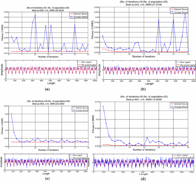
Procedure of iterations and effect of de-noising. a additive noise levels: 10%, b additive noise levels: 20%, c additive noise levels: 50%, d additive noise levels: 100%

The effect of de-noising is illustrated in Table 1. The increment of SNR for the four situations is about 15–20 dB. It is seen that the row number p is almost half of the length of data, which means that the Hankel matrix is nearly a square matrix. The effective rank r is 4, which is twice the number of frequency components.
For numerical case I, the length data is 1024, which is suitable for numerical study. But for real measurements of civil structures, it usually need to do data collection for more than 20 min. In order to get better effect of de-noising, for this huge amounts of data, is it necessary to construct a square Hankel matrix? It might take us a couple of days for computing. The second situation, which is disturbed by 50% additive noise level, is under investigated here. The effective rank r is set to be 4. Row number p is set to be from 50 to 900, with a increment step of 50. Figure 6 shows that in the range of 200–800 (\(p \approx [N/5,\;2N/3]\)), we get very close results, which means that SNRs of de-noised signal are almost about 23 dB. So, for improving the calculating efficiency, a rectangular matrix with appropriate selection of row number p is large enough to represent the system behavior including the effect of noise.

Effect of de-noising under the situation: k = 4, p = 200–800
4.3 Numerical study: case II
In case I, the simulated signal with two frequency components was disturbed by Gaussian white noise. As affected by the violent background vibration or the strong environmental electromagnetic disturbances, the signals collected from field are often inevitably contaminated by not only Gaussian white noise, but also non-Gaussian colored noise. Additionally, for vibration-based SHM, we usually care about the first few frequencies [39, 40]. In case II, the following simulated signal is considered
where \(f_{1} = 0.5\;{\text{Hz}}\), \(f_{2} = 1.5\;{\text{Hz}}\), \(f_{3} = 2.5\;{\text{Hz}}\), \(f_{4} = 5\;{\text{Hz}}\), \(f_{5} = 10\;{\text{Hz}}\); \(e_{1} (t)\) represents the Gaussian white noise, \(\alpha\) indicates 50% noise level; \(e_{2} (t)\) represents colored noise with bandwidth of [0.2–20] Hz; \(e_{3} (t)\) represents impulse noise; the length N of the simulated signal above is chosen as 1024.
SNR of the mixed signal is − 5.5742 dB, which indicates that the power of noise is greater than the power of pure signal. Distribution of Singular Entropy is illustrated in Fig. 7, which shows an asymptote after the 20th singular values. Using GA–SVD approach, the range of effective rank r is set to be in the range of [4, 20], the range of row number p is set to be in the range of [N/10, N/2]. Procedure of iteration is shown in Fig. 8. SNR of the de-noised signal is 6.1388 dB, which illustrates that the noise has been weakened greatly. The row number p = 413 (about N/3), effective rank r = 10 (twice the number of frequency components). Figure 9 shows a pure signal in red color, which is so clear that the waveform can be distinguished from noise. The five frequency components can be identified accurately by peak picking method.

Distribution of Singular Entropy

Procedure of iterations

Effect of de-noising
It is worth noted that, from the results of case I and II: (1) effective rank can be defined as twice the number of frequency components; (2) row number p can be defined in the range of [N/5, 2 N/3], which is < N/2. For real measurements of civil structures, it usually need to do data collection for > 20 min. So we can defined row number p as N/4 or N/3, which construct a rectangular matrix and less computations are needed.
4.4 Experimental study
An operational modal test was conducted in 2011, for a long span cable-stayed bridge, whose span combination is 165 m + 338 m + 165 m, Fig. 10. For vertical vibration modal test, the sampling frequency was set to 160 Hz, each group of data lasts for about 20 min. At first, we must confirm the modes that we care about. From the analysis of Finite Element Model (FEM), it is known that the first 15 modes are < 5 Hz, who are usually used for SHM. Secondary, the data was resampled at 12 Hz. The data of the first 170 s was chosen for analyzing, whose length is 2048. FFT was conducted to the raw acceleration data, the spectrogram illustrated in Fig. 11 that: (1) the first three natural frequencies are obviously to identified by the peaks in the range of [0, 1] Hz; (2) in the range of [1, 2] Hz, the peaks are not so obvious. The identification accuracy is determined by frequency resolution; (3) in the range of [2, 6] Hz, the peaks are too messy to identified.

Experimental study: Yamen bridge. a Finite element mode, b modal test of vertical vibration

Raw acceleration data and spectrogram
Using GA–SVD, row number p was set as 512 (N/4) to construct Hankel matrix. Distribution of Singular Entropy was illustrated in Fig. 12. From the analysis of FEM, it is known that there are 15 modes in the range of [0, 5] Hz. According to the conclusion of numerical studies above, the effective rank r should be as twice the number of frequency components. But for this field measurement data, some real modal frequency will be filtered if effective rank r is set as 30. When row number p was set as 512 and effective rank r is set as 40, it is obvious that better result will be gotten. So when dealing with real measurements, effective rank r should be greater than twice the number of frequency components.

Distribution of Singular Entropy
Eigensystem Realization Algorithm was applied to identify modal parameters based on the de-noised signal. As shown in Table 2 and Fig. 13, the first six modes identified are in great agreement with [40], which can reflect the real dynamic characteristic of the structure, though there are closely spaced modes in the range of [0, 2] Hz.

Spectrogram of raw signal and de-noised signal
5 Conclusion
An adaptive approach for noise reduction is proposed which based on GA and SVD. Both the row number of Hankel matrix p and effective rank r are difficult to determine for noise reduction based on SVD. For the adaptive approach, GA is applied to determine the two key parameters adaptively. In order to demonstrate the validity of the approach, two numerical simulation signals with different frequency components are employed. The results show that p can be N/4 or N/3 (N is the length of data), r is twice as the number of dominating frequency. As for measured signal, the complication of the frequency components might be taken into consideration. And in order not to miss the real frequency components when dealing with measured signals, r should be more than twice as the number of dominating frequency, but p can still be N/4 so that no additional computation is needed.
References
Janacek, G.J.: Practical Time Series. Arnold, London (2001)
Shumway, R.H., Stoffer, D.S.: Time Series Analysis and Its Applications. Springer, New York (2000)
Kim, Y.Y., Hong, J.C., Lee, N.Y.: Frequency response function estimation via a robust wavelet de-noising method. J. Sound Vib. 244(4), 635–649 (2001)
Lin, J.-W., Laine, A.F., Bergmann, S.R.: Improving PET-based physiology quantification through methods of wavelet denoising. IEEE Trans. Biomed Eng. 48(2), 202–212 (2001)
Shim, I., Soraghan, J.J., Siew, W.H.: Noise reduction technique for on-line detection and location of partial discharges in high voltage cable. Meas. Sci. Technol. 11(12), 1708–1713 (2000)
Presti, L.L., Olmo, G., Bosetto, D.: Turbo estimation algorithms: general principles, and applications to modal analysis. Signal Process. 80(12), 2567–2578 (2000)
Leibrich, J., Puder, H.: A “TF distribution for disturbed and undisturbed speech signals and its application to noise reduction”. Signal Process. 80(9), 1761–1776 (2000)
Jeff, L., Rafik, G.: GMDF for noise reduction and echo cancellation. IEEE Signal Process. Lett. 7(8), 230–232 (2000)
Gharieb, R.R., Cichocki, A.: Noise reduction in bra third-or. IEEE Trans. Biomed. Eng. 48(5), 501–512 (2001)
Muneyasu, M., Nishi, N., Hinamoto, T.: A new adaptive center weighted median filter using counter propagation networks. J. Franklin Inst. 337(5), 631–639 (2000)
Kitamura, K., Iida, H., Shidahara, M., Miura, S., Kanno, I.: Noise reduction in PET attenuation correction using non-linear Gaussian filters. IEEE Trans. Nucl. Sci. 47(3), 994–999 (2000)
Sakitani, K., Maeda, H.: Optimum noise reduction of conjugate quadrature filter bank. Signal Process. 8(5), 819–829 (2000)
Laakso, T.I., Tarczynski, A., Paul Murphy, N., Valimaki, V.: Polynomial filtering approach to reconstruction and noise reduction of nonuniformly sampled signals. Signal Process. 80(4), 567–575 (2000)
Gialamas, T.P., Tsahalis, D.T., Otte, D., Van der Auwaraer, H., Manolas, D.A.: Substructuring techniques: improvement by means of singular value decomposition (SVD). Appl. Acoust. 62(10), 1211–1219 (2001)
Kim, W.C., Chin, I.S., Lee, K.S., Choi, J.: Analysis and reduced-order design of quadratic criterion-based iterative learning control using singular value decomposition. Comput. Chem. Eng. 24(8), 1815–1819 (2000)
Ray, G., Prasad, A.N., Bhattacharyya, T.K.: Design of decentralized robust load–frequency controller based on SVD method. Comput. Electr. Eng. 25(6), 477–492 (1999)
Street, A.M., Lukama, L., Edwards, D.J.: Radio imaging using SVD prony. Electron. Lett. 36(13), 1150–1152 (2000)
Vidya, V., Aravena, Jorge L.: Nonstationary signal classification using pseudo power signatures: the matrix SVD approach. IEEE Trans. Circuits Syst. II 46(12), 1497–1505 (1999)
Dale, G., David, B.: Feature sets for nonstationary signals derived from moments of the singular value decomposition of Cohen-Posch (positive time–frequency) distributions. IEEE Trans. Signal Process. 48(5), 1498–1503 (2000)
Knockaert, L., De Backer, B., De Zutter, D.: SVD compression, unitary transforms, and computational complexity. IEEE Trans. Signal Process. 47(10), 2724–2729 (1999)
Kuo, S.R., Yeih, W., Wu, Y.C.: Applications of the generalized singular value decomposition method on the eigenproblem using the incomplete boundary element formulation. J. Sound Vib. 235(5), 813–845 (2000)
Chen, J.T., Huang, C.X., Wong, F.C.: Determination of spurious eigenvalue and multiplicities of true eigenvalues in the dual multiple reciprocity method using the singular-value decomposition technique. J. Sound Vib. 230(2), 203–219 (2000)
Pau, J.S., Reddy, M.R., Kumar, V.J.: A transform domain SVD filter for suppression of muscle noise artifacts in exercise ECG’s. IEEE Trans. Biomed. Eng. 47(5), 654–663 (2000)
Kanjilal, P.P., Palit, S.: On multiple pattern extraction using singular value decomposition. IEEE Trans. Signal Process. 43(6), 1536–1540 (1995)
Vautard, R., Yiou, P., Ghil, M.: Singular-spectrum analysis: a toolkit for short, noisy chaotic signals. Physica D 58(1–4), 95–126 (1992)
Yang, W.X., Peter, W.T.: Development of an Advanced Noise Reduction Method for Vibration Analysis Based on Singular Value Decomposition. NDT and E Int. 36(6), 419–432 (2003)
Konstantinides, K., Yao, K.: Statistical analysis of effective singular values in matrix rank determination. IEEE Trans. Acousti. Speech Signal Process. 36(5), 757–763 (1988)
Cakar, O., Sanliturk, K.Y.: Elimination of noise and transducer effects from measured response data. In Proceedings of ESDA2002: 6th Biennial Conference on Engineering Systems Design and Analysis, Istanbul (2002)
Zhao, X., Ye, B.: Similarity of signal processing effect between Hankel matrix-based SVD and wavelet transform and its mechanism analysis. Mech. Syst. Signal Process. 23(4), 1062–1075 (2009)
Zhu, Q.B., Liu, J., Li, Y.G.: Study on noise reduction in singular value decomposition based on structural risk minimization. J. Vib. Eng. 18(2), 204–207 (2005). (in Chinese)
Wang, W., Zhang, Y.T., Xu, Z.S.: Noise reduction in singular value decomposition based on dynamic clustering. J. Vib. Eng. 21(3), 304–308 (2008). (in Chinese)
Chunyu, K.: ZHANG Xinhua “An adaptive noise reduction method based on singularity value decompose”. Tech. Acoust. 27(3), 455–458 (2008). (in Chinese)
Konstantinides, K., Natarajan, B., Yovanof, G.S.: Noise estimation and filtering using block-based singular value decomposition. IEEE Trans. Image Process. 6(3), 283–479 (1997)
Hou, Z.: Adaptive singular value decomposition in wavelet domain for image denosing. Pattern Recogn. 36(8), 1747–1763 (2003)
Brenner, M.J.: Non-stationary dynamic data analysis with wavelet-SVD filtering. Mech. Syst. Signal Process. 17(4), 765–786 (2003)
Duan, L.X., Zhang, L.B., Wang, Z.H.: De-noising of diesel vibration signal using wavelet packet and singular value decomposition. Front. Mech. Eng. China 1(4), 443–447 (2006)
Golub, G.H., Van Loan, C.F.: Matrix Computations, 2nd edn. John Hopkins University Press, Baltimore (1989)
Jensen, S.H., Hansen, P.C., et al.: Reduction of broad-band noise in speech by truncated QSVD. IEEE Trans. Speech Audio Process. 3(6), 439–448 (1995)
Holland, J.H.: Adaptation in Natural and Artificial Systems: an Introductory Analysis with Applications to Biology, Control, and Artificial Intelligence. University of Michigan Press, Michigan (1975)
Xi-Jun, Y.E., Yan, Q.S., Jian, L.I.: Modal identification and cable tension estimation of long span cable-stayed bridge based on ambient excitation. J. Vib. Shock 31(16), 157–163 (2012). (in Chinese)
Acknowledgements
This work was supported in part by the National Natural Science Foundation of China under Grant No. 51608136 and Research project of Guangdong Provincial Highway Administration Bureau (No. 2017-1).
Author information
Authors and Affiliations
Corresponding author
Ethics declarations
Conflict of interest
The authors confirm that this article content has no conflict of interest.
Rights and permissions
About this article

Cite this article
Ye, X., Sun, Z. & Chen, B. Research on modal parameters identification of bridge structure based on adaptive signal de-noising method. Cluster Comput 22 (Suppl 6), 14377–14387 (2019). https://doi.org/10.1007/s10586-018-2301-1
Received:
Revised:
Accepted:
Published:
Issue Date:
DOI: https://doi.org/10.1007/s10586-018-2301-1