Strange star admitting Chaplygin equation of state in Finch–Skea spacetime

Abstract

In the present paper we propose a new model of an anisotropic strange star which admits the Chaplygin equation of state. The exterior spacetime is described by a Schwarzschild line element. The model is developed by assuming the Finch–Skea ansatz (Finch and Skea in Class. Quantum Gravity 6:467, 1989). We obtain the model parameters in closed form. Our model is free from a central singularity. Choosing some particular values for the parameter we show that our model corroborates the observational data of the strange star PSR J1614-2230 (Gangopadhyay et al. in Mon. Not. R. Astron. Soc. 431:3216, 2013).

1 Introduction

Studies of relativistic models of compact stars have been an intersecting topic to researchers for the last few decades. The possible compact objects are strange stars and neutron stars. Strange stars are composed of quarks or strange matter consisting of u, d, and s quarks, whereas on the other hand neutron stars are composed of neutrons. The formation of strange matter can be classified into two ways: the quark–hadron phase transition in the early universe and conversion of neutron stars into strange stars at ultrahigh densities (Witten 1984). Bodmer (1971) proposed that a phase transition between hadronic and strange quark matter may occur in the universe at a density higher than the nuclear density when a massive star explodes as a supernova. So one expects to find the strange quark at the inner core of a neutron star or a quark star. According to Ruderman (1972) the pressure inside the highly compact astrophysical objects like an X-ray pulsar, Her-X-1, X-ray buster 4U 1820-30, the millisecond pulsar SAX J 1804.4-3658, PSR J1614-2230, LMC X-4 etc. that have a core density beyond the nuclear density $(10^{15}~\mbox{gm}/\mbox{cc})$ show anisotropy , i.e., the pressure inside these compact objects can be decomposed into two parts: the radial pressure $p_{r}$ and the transverse pressure $p_{t}$ where $p_{t}$ is in the direction perpendicular to $p_{r}$. $\Delta=p_{t}-p_{r}$ is called the anisotropic factor. The reasons behind these anisotropic nature are the existence of a solid core, the presence of a type $P$ superfluid, a phase transition, a rotation, a magnetic field, a mixture of two fluids, the existence of an external field, etc. Local anisotropy in self-gravitating systems was studied by Herrera and Santos (1997) (please, see the references therein for a review of anisotropic fluids). A large number of works have been done earlier by assuming an anisotropic pressure of the underlying fluid. By assuming a special type of matter density Dev and Gleiser (2004) proposed a model of an anisotropic star. From their analysis the authors have shown that the absolute stability bound $\frac{2M}{R}<\frac{8}{9}$ can be violated and the star’s surface redshift may be arbitrarily large. A strange star in Krori–Barua spacetime is described by Rahaman et al. (2011). A strange quintessence star and a singularity free quintessence star in Krori–Barua spacetime are obtained by Bhar (2015a,b). A new class of interior solutions of a ($2+1$)-dimensional anisotropic star in a Finch–Skea spacetime corresponding to the exterior BTZ black hole was developed by Bhar et al. (2014). The model is obtained by considering the MIT bag model equation of state, and a particular ansatz for the metric function $g_{rr}$ was proposed by Finch and Skea (1989). A relativistic stellar model admitting a quadratic equation of state was proposed by Sharma and Ratanpal (2013) in a Finch–Skea spacetime. The earlier work is generalized to a modified Finch–Skea spacetime by Pandya et al. (2014) by incorporating a dimensionless parameter n. In a very recent work Bhar (2015) obtained a new model of an anisotropic superdense star which admits conformal motions in the presence of a quintessence field which is characterized by a parameter $\omega_{q}$ with $-1 < \omega_{q} < -1/3$. The model has been developed by choosing the ansatz from Vaidya and Tikekar (1982). One of the most important discoveries in the recent past is that the expansion of our universe is accelerating, which is observed by Type Ia supernovae (Riess et al. 1998; Perlmutter et al. 1999). Dark energy is the most useful hypothesis to explain this phenomenon. As a result the Chaplygin gas EOS is very useful in order to explain the accelerating phase of our present universe as well as to unify the dark energy and dark matter. As the Chaplygin gas EOS is a specific form of polytropic EOS, it describes dark energy. On the other hand, it is believed that dark energy exerts a repulsive force on its surrounding, which prevents the star from gravitational collapse in the same manner as an electric charge. Lobo (2006) has given a model of a stable dark energy star by assuming two spatial types of mass function: one is of constant energy density and the other mass function is Matese and Whitman (1980) a constant mass. All the features of the dark energy star have been discussed and the system is stable under a small linear perturbation. Very recently Bhar and Rahaman (2015) proposed a new model of a dark energy star consisting of five zones, namely, a solid core of constant energy density, a thin shell between core and interior, an inhomogeneous interior region with anisotropic pressures, a thin shell, and an exterior vacuum region. They discussed various physical properties. The model satisfies all the physical requirements. The stability condition under a small linear perturbation is also discussed. The generalized Chaplygin gas model is based on the equation of state $P_{ch}=-\frac{A}{\rho_{ch}^{\alpha}}$ where $A$ and $\alpha$ are positive constants and $0 \leq\alpha\leq1$. Bertolami and Paramos (2005) studied the general properties of a spherically symmetric body described through the generalized Chaplygin equation of state. They conclude that such an object, dubbed a generalized Chaplygin dark star, should exist within the context of the generalized Chaplygin gas (GCG) model of the unification of dark energy and dark matter, and they derive expressions for its size and expansion velocity, whereas Rahaman et al. (2010) have described anisotropic charged fluids with a Chaplygin equation of state. In this paper the authors deal with a nonlinear EOS and are able to find solutions using an algebraic method without solving any differential equations. Gorini et al. (2009) investigate the Tolman–Oppenheimer–Volkoff equations for the generalized Chaplygin gas with the aim of extending their earlier work (Gorini et al. 2008), where the authors studied static solutions of the Tolman–Oppenheimer–Volkoff equations for spherically symmetric objects (stars) living in a space filled with the Chaplygin gas. The modified Chaplygin gas (MCG) EoS for the radial pressure is described by $p_{r}(r) = A\rho(r)-\frac{B}{\rho(r)^{\alpha}}$. Here $A$, $B$, and $\alpha$ are constant parameters. Mubasher et al. (2009) constructed a stationary, spherically symmetric, and spatially inhomogeneous wormhole spacetime supported by a modified Chaplygin gas. In particular, if we take $\alpha =1$ we get the Chaplygin equation of state. Inspired by all of the previous works, in the present paper we want to model an anisotropic star in a Finch–Skea spacetime incorporating the Chaplygin equation of state. Our paper is planned as follows: In Sect. 2 we discuss the Einstein field equations. The solutions of the system are treated in Sect. 3. The other features are given in Sects. 4–10, and finally some concluding remarks are given in Sect. 11.

2 Einstein field equations

To describe the interior of a static spherically symmetry distribution of matter the line element is given by

$$ ds^{2}=-e^{\nu(r)}\,dt^{2}+e^{\lambda(r)}\,dr^{2}+r^{2} \bigl(d\theta^{2}+\sin ^{2}\theta \,d\phi^{2}\bigr) $$

(1)

in Schwarzschild co-ordinates $x^{a}=t, r, \theta, \phi$. Here $\lambda$ and $\nu$ are functions of the radial co-ordinate $r$ only. Let us assume that the matter distribution inside the compact star is anisotropic in nature, whose energy momentum tensor is given by the following equation:

$$ T_{\nu}^{\mu}=(\rho+p_{r})u^{\mu}u_{\nu}-p_{t} g_{\nu}^{\mu}+(p_{r}-p_{t})\eta ^{\mu}\eta_{\nu} $$

(2)

with $u^{i}u_{j} =-\eta^{i}\eta_{j}= 1$ and $u^{i}\eta_{j}= 0$. Here the vector $u_{i}$ is the fluid 4-velocity and $\eta^{i}$ is the spacelike vector which is orthogonal to $u_{i}$, $\rho$ is the matter density, $p_{r}$ and $p_{t}$ are, respectively, the radial and the transversal pressure of the fluid and $p_{t}$ lies in the direction orthogonal to $p_{r}$.

Taking $G = 1 = c$ the Einstein field equations can be written as

$$\begin{aligned}& 8\pi\rho=\frac{1}{r^{2}} \bigl[r\bigl(1-e^{-2\lambda}\bigr) \bigr]', \end{aligned}$$

(3)

$$\begin{aligned}& 8\pi p_{r}=-\frac{1}{r^{2}}\bigl(1-e^{-2\lambda}\bigr)+ \frac{2\nu' }{r}e^{-2\lambda}, \end{aligned}$$

(4)

$$\begin{aligned}& 8\pi p_{t}=e^{-2\lambda} \biggl(\nu''+ \nu^{\prime\,2}+\frac{\nu '}{r}-\nu'\lambda'- \frac{\lambda'}{r} \biggr). \end{aligned}$$

(5)

Here a prime denotes differentiation with respect to the radial co-ordinate $r$. Now the mass contained within the sphere of radius $r$ is given by

$$ m(r)=\int_{0}^{r}4\pi\rho(\omega) \omega^{2}\,d\omega. $$

(6)

We assume that the radial pressure ($p_{r}$) and the matter density $\rho$ are related as (Benaoum 2002)

$$ p_{r}=\alpha_{1} \rho+\frac{\alpha_{2}}{\rho}. $$

(7)

Here $\alpha_{1}$ and $\alpha_{2}$ are some constants. The above equation is known as the generalized Chaplygin gas equation of state for the fluid sphere. Now let us introduce the transformation

$$ x=r^{2},\quad Z(x)=e^{-2\lambda(r)}\quad\mbox{and}\quad y^{2}(x)=e^{2\nu(r)}. $$

(8)

Using this transformation Einstein field equations become

$$\begin{aligned}& 8\pi\rho=\frac{1-Z}{x}-2\dot{Z}, \end{aligned}$$

(9)

$$\begin{aligned}& 8\pi p_{r}=4Z\frac{\dot{y}}{y}+\frac{Z-1}{x}, \end{aligned}$$

(10)

$$\begin{aligned}& p_{t}= p_{r}+\Delta, \end{aligned}$$

(11)

$$\begin{aligned}& 8\pi\Delta=4xZ\frac{\ddot{y}}{y}+\dot{Z} \biggl(1+2x\frac{\dot {y}}{y} \biggr)+ \frac{1-Z}{x}. \end{aligned}$$

(12)

Using Eqs. (7), (9), and (10) we obtain

$$\begin{aligned} \frac{\dot{y}}{y} =&\frac{\alpha_{1}}{4Z} \biggl(\frac{1-Z}{x}-2\dot{Z} \biggr)+\frac{\alpha_{2}}{4Z}(8\pi)^{2} \biggl(\frac{1-Z}{x}-2\dot{Z} \biggr)^{-1} \\ &{}-\frac{Z-1}{4Zx}. \end{aligned}$$

(13)

Here a dot denotes the derivative with respect to $x$. The mass function becomes

$$ m(x)=2\pi\int_{0}^{x}\sqrt{\omega}\rho(\omega)\,d \omega. $$

(14)

3 Solution

To solve the Einstein field equations let us take the ansatz proposed by Finch and Skea (1989):

$$ e^{2\lambda}=1+\frac{r^{2}}{R^{2}}. $$

(15)

Using Eqs. (8) and (15) we get

$$ Z(x)=(1+ax)^{-1}. $$

(16)

Here $a=\frac{1}{R^{2}}$. Using the expression of $Z(x)$ from Eqs. (9)–(13) we obtain

$$ \frac{\dot{y}}{y}=\frac{\alpha_{1} a}{4}\frac{3+ax}{1+ax}+(8\pi)^{2} \frac {\alpha_{2}}{4a}\frac{(1+ax)^{3}}{3+ax}+\frac{a}{4}. $$

(17)

Integrating the above equations we get

$$\begin{aligned}& \ln(y)=\frac{\alpha_{1}}{4}\bigl[ax+2\ln(1+ax)\bigr]+\frac{ax}{4} \\ & \phantom{\ln(y)=\,\,}{} +\frac{(8\pi)^{2}\alpha_{2}}{4a^{2}} \biggl[\frac {(3+ax)^{3}}{3}-3(3+ax)^{2} \biggr] \\ & \phantom{\ln(y)=\,\,}{}+ \frac{(8\pi)^{2}\alpha_{2}}{4a^{2}} \bigl[12ax-8\ln(3+ax) \bigr]+C, \end{aligned}$$

where $C$ is the constant of integration, which will be determined from the boundary condition. The matter density and the radial and transverse pressure are obtained as

$$\begin{aligned}& \rho=\frac{3a+a^{2}x}{8\pi(1+ax)^{2}}, \end{aligned}$$

(18)

$$\begin{aligned}& p_{r}=\alpha_{1} \rho+\frac{\alpha_{2}}{\rho}, \end{aligned}$$

(19)

$$\begin{aligned}& p_{t}=p_{r}+\Delta, \end{aligned}$$

(20)

and the anisotropic factor $\Delta$ is obtained as

$$\begin{aligned} 8\pi\Delta =&4x \biggl\{ \frac{\alpha_{1} a}{4}\frac{3+ax}{(1+ax)^{2}}+\frac {(8\pi)^{2}\alpha_{2}}{4a} \frac{(1+ax)^{2}}{3+ax} \biggr\} \\ &{}\times \biggl\{ \frac{\alpha_{1} a}{4}\frac{3+ax}{(1+ax)^{2}}+\frac{(8\pi )^{2}\alpha_{2}}{4a} \frac{(1+ax)^{2}}{3+ax} +\frac{a}{4} \biggr\} \\ &{}+4x \biggl\{ \frac{(8\pi)^{2}\alpha_{2}}{2}\frac {(1+ax)(4+ax)}{(3+ax)^{2}}-\frac{\alpha_{1}a^{2}}{2(1+ax)^{3}} \biggr\} \\ &{}-2ax \biggl[\frac{\alpha_{1}a}{4}\frac{3+ax}{(1+ax)^{3}}+\frac{(8\pi )^{2}\alpha_{2}}{4a} \frac{1+ax}{3+ax}\\ &{}+\frac{a}{4(1+ax)^{2}} \biggr] -\frac{a}{(1+ax)^{2}}+\frac{a}{1+ax}. \end{aligned}$$

4 Exterior spacetime and matching condition

In this section we match our interior solution to the exterior Schwarzschild metric at the boundary $r = r_{b}$ where $r_{b} > 2M$. The exterior spacetime is given by the line element

$$\begin{aligned} ds^{2} =&- \biggl(1-\frac{2M}{r} \biggr)dt^{2}+ \biggl(1-\frac{2M}{r} \biggr)dr^{2} \\ &{} +r^{2}\bigl(d\theta^{2}+\sin^{2} \theta d\phi^{2}\bigr). \end{aligned}$$

(21)

Now at the boundary $r = r_{b}$ the coefficients of $g_{rr}$, $g_{tt}$ all are continuous. This implies

$$\begin{aligned}& 1-\frac{2M}{r_{b}}=e^{2\nu(r_{b})} \end{aligned}$$

(22)

$$\begin{aligned}& \biggl(1-\frac{2M}{r_{b}} \biggr)^{-1}=1+ar_{b}^{2}. \end{aligned}$$

(23)

From Eq. (22) we obtain

$$\begin{aligned} C =&\frac{1}{2}\ln \biggl(1-\frac{2M}{r_{b}} \biggr)-\frac{\alpha _{1}}{4} \bigl[ar_{b}^{2}+2\ln\bigl(1+ar_{b}^{2} \bigr)\bigr]-\frac{ar_{b}^{2}}{4} \\ &{} -\frac{(8\pi)^{2}\alpha_{2}}{4a^{2}} \biggl[\frac {(3+ar_{b}^{2})^{3}}{3}-3\bigl(3+ar_{b}^{2} \bigr)^{2} \biggr] \\ &{} -\frac{(8\pi)^{2}\alpha_{2}}{4a^{2}} \bigl[12ar_{b}^{2}-8\ln \bigl(3+ar_{b}^{2}\bigr) \bigr]. \end{aligned}$$

(24)

5 Physical analysis

• (1) The matter density ($\rho$) and the radial pressure ($p_{r}$) should be non-negative inside the stellar interior. The profile of $\rho$ and $p_{r}$ are shown in Figs. 1 and 2, respectively. From the figures it is clear that our proposed model of a strange star satisfies this condition. At the boundary of the star the radial pressure vanishes.

  Fig. 1

  

  The variation of matter density $\rho$ is plotted against $r$ inside the stellar interior

  Fig. 2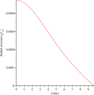

  

  The variation of the radial pressure $p_{r}$ is plotted against $r$ inside the stellar interior

• (2) Both $\frac{d\rho}{dr}$ and $\frac{dp_{r}}{dr}~<0$ (see Fig. 4), i.e., $\rho$ and $p_{r}$ are monotonic decreasing functions of $r$, they have a maximum value at the center of the star and they decrease radially outwards.

• (3) For an anisotropic fluid sphere the trace of the energy tensor should be positive, as suggested by Bondi (1999). To check this condition for our model we plot $\rho- p_{r} - 2p_{t}$ against $r$ in Fig. 5. From the figure it is clear that $\rho- p_{r} - 2p_{t} \geq0$.

• (4) The profile of the anisotropic factor $\Delta= p_{t} - p_{r}$ is shown in Fig. 3. The anisotropic factor $\Delta< 0$ for our model. So the anisotropic force is attractive in nature and at the center of the star the anisotropic factor vanishes, which is expected.

  Fig. 3

  

  The variation of the anisotropic factor $\Delta=p_{t}-p_{r}$ is shown against $r$ inside the stellar interior

  Fig. 4

  

  $\frac{d\rho}{dr}$, $\frac{dp_{r}}{dr}$ are plotted against $r$ inside the stellar interior

  Fig. 5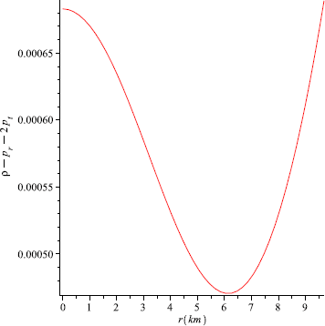

  

  The variation of $\rho-p_{r}-2p_{t}$ is plotted against $r$ inside the stellar interior

• (5) Moreover, for an anisotropic fluid sphere the radial and transverse velocity of sound should be less than 1, which is known as a causality condition. This condition is discussed separately in Sect. 7.

6 Adiabatic index

For an anisotropic fluid sphere the adiabatic index ($\gamma$) is given by

$$ \gamma=\frac{\rho+p_{r}}{p_{r}}\frac{dp_{r}}{d\rho}. $$

(25)

Heintzmann and Hillebrandt (1975) proposed that a neutron star with an anisotropic equation of state will be stable if $\gamma>\frac{4}{3}$. To see the characteristics of the adiabatic index for our model the profile is shown in Fig. 6. From the figure we see that $\gamma>\frac{4}{3}$ everywhere within the interior of the fluid sphere. So according to Heintzmann and Hillebrandt (1975) our model is stable.

Fig. 6

The adiabatic index $\gamma$ (green curve) is shown against $r$ inside the stellar interior and the red line corresponds to $r=\frac {4}{3}$

7 Stability

Our proposed model of an anisotropic strange star will be physically acceptable if the radial and transverse velocity of sound should be less than 1, which is known as a causality condition. Here the radial velocity $(v_{sr}^{2})$ and the transverse velocity $(v_{st}^{2})$ of sound can be obtained as

$$\begin{aligned}& v_{sr}^{2}=\frac{dp_{r}}{d\rho}, \end{aligned}$$

(26)

$$\begin{aligned}& v_{st}^{2}=\frac{dp_{t}}{d\rho}. \end{aligned}$$

(27)

As regards the complexity of the expression of $p_{t}$ we prove the above inequalities with the help of a graphical representation. The profiles of $v_{sr}^{2}$ and $v_{st}^{2}$ are shown in Figs. 7 and 8. From these two figures it is clear that $0< v_{sr}^{2}$, $v_{st}^{2}\leq 1$ everywhere within the anisotropic fluid sphere. Moreover, $0< v_{sr}^{2}<1$, $0< v_{st}^{2}<1$, therefore, according to Andreasson (2009) $|v_{sr}^{2}-v_{st}^{2}|<1$, which is also satisfied by our model (see Fig. 9).

Fig. 7

The variation of radial velocity is shown against $r$ inside the stellar interior

Fig. 8

The variation of transverse velocity is shown against $r$ inside the stellar interior

Fig. 9

$\vert {-}v_{st}^{2}+v_{sr}^{2}\vert$ is shown against $r$ inside the stellar interior

8 TOV equation

To check whether our model is in equilibrium under the three different forces, we consider the generalized Tolman–Oppenheimer–Volkov (TOV) equation which is represented by the formula

$$ \frac{M_{G}(\rho+p_{r})}{r^{2}}e^{\frac{\lambda-\nu}{2}}+\frac {dp_{r}}{dr}+\frac{2}{r}(p_{t}-p_{r}). $$

(28)

Here $M_{G} = M_{G}(r)$ is the effective gravitational mass inside the fluid sphere of radius $r$ defined by

$$ M_{G}(r)=\frac{1}{2}r^{2}e^{\frac{\nu-\lambda}{2}} \nu'. $$

(29)

The above expression of $M_{G}(r)$ can be derived from the Tolman–Whittaker mass formula. Using the expression of Eq. (29) in (28) we obtain the modified TOV equation as

$$ F_{g}+F_{h}+F_{a}=0, $$

(30)

where

$$\begin{aligned}& F_{g}=-\frac{\nu'}{2}(\rho+p_{r}), \end{aligned}$$

(31)

$$\begin{aligned}& F_{h}=-\frac{dp_{r}}{dr}, \end{aligned}$$

(32)

$$\begin{aligned}& F_{a}=\frac{2}{r}(p_{t}-p_{r}); \end{aligned}$$

(33)

$F_{g}$, $F_{h}$, and $F_{a}$ are known as gravitational, hydrostatic, and anisotropic forces, respectively, of the system. The profiles of the above three forces for the strange star are shown in Fig. 10. This figure shows that the combined effect of hydrostatic and anisotropic forces are counterbalanced by the gravitational forces. So the present system is in static equilibrium under these three forces.

Fig. 10

The variation of gravitational, hydrostatic, and anisotropic forces are shown against $r$ inside the stellar interior

9 Energy condition

In this section we want to check whether our model of an anisotropic strange star satisfies all the energy conditions. It is well known that for an anisotropic fluid sphere all the energy conditions, namely the Weak Energy Condition (WEC), the Null Energy Condition (NEC) and the Strong Energy Condition (SEC) are satisfied if and only if the following inequalities hold simultaneously for every point inside the fluid sphere:

$$\begin{aligned}& \mbox{NEC}:\quad\rho+p_{r}\geq0, \end{aligned}$$

(34)

$$\begin{aligned}& \mbox{WEC}:\quad p_{r}+\rho\geq0,\quad \rho>0, \end{aligned}$$

(35)

$$\begin{aligned}& \mbox{SEC}:\quad\rho+p_{r}\geq0, \quad \rho+p_{r}+2p_{t} \geq0. \end{aligned}$$

(36)

As regards the complexity of the expression of $p_{t}$ we will prove the above inequalities with the help of a graphical representation. The l.h.s. of the above inequalities are plotted in Fig. 11. The figure shows that all the energy conditions are satisfied by our model of anisotropic strange star.

Fig. 11

Energy conditions are shown against $r$ inside the stellar interior

10 Some features

10.1 Mass of the strange star

The total mass of the anisotropic star within the radius $r$ can be obtained as

$$ M=\int_{0}^{r}4\pi r^{2}\rho \,dr= \frac{ar^{3}}{2(1+ar^{2})}. $$

(37)

The profile of the mass function is shown in Fig. 12. The mass function is regular at the center of the star since as $r\rightarrow0$, $m(r)\rightarrow0$. Moreover, the mass function is a monotonic increasing function of $r$ and it is positive inside the stellar configuration.

Fig. 12

The variation of the mass function is shown against $r$

11 Compactness

The ratio of the mass to the radius of a strange star, known as the compactification factor, cannot be arbitrarily large. Buchdahl (1959) showed that for a ($3+1$)-dimensional fluid sphere $\frac{2M}{r_{b}}<\frac{8}{9}$. To see the maximum allowable ratio of mass to the radius for our model we calculate the compactness of the star given by

$$ u=\frac{m(r)}{r}=\frac{ar^{2}}{2(1+ar^{2})}. $$

(38)

The profile of $u(r)$ is shown in Fig. 13. The figure shows that $u(r)$ is a monotonic increasing function of $r$. To see twice the maximum allowable ratio of the mass to the radius we have calculated the values of $\frac{2m}{r_{b}}= 0.618$ from our model of strange star, which lies in the expected range of (Buchdahl 1959).

Fig. 13

The compactification factor is shown against $r$ inside the stellar interior

12 Surface redshift

The surface redshift function $z_{s}$ of our model of a strange star is defined by

$$ 1+z_{s}=(1-2u)^{-\frac{1}{2}}. $$

(39)

Therefore, the surface redshift function $z_{s}$ can be obtained as

$$ z_{s}= \biggl(\frac{1}{1+ar^{2}} \biggr)^{-\frac{1}{2}}-1. $$

(40)

The profile of the surface redshift is shown in Fig. 14. The maximum value of the surface redshift for our model of a strange star is obtained as 0.629.

Fig. 14

The surface redshift is shown against $r$ inside the stellar interior

13 Discussion and concluding remarks

In the present paper we have solved the Einstein field equations in closed form by choosing the Chaplygin equation of state. The model is developed by choosing the Finch–Skea ansatz. Our model is free from central singularities. The model parameters $\rho$, $p_{r}$ are nonnegative and monotonic decreasing function of $r$, i.e., they have a maximum value at the center of the star and it decreases radially outward inside the stellar interior. By choosing some reasonable values for the parameters we obtain the central density of the star to be $2.84 \times10^{15}~\mbox{gm}/\mbox{cc}$. The pressure anisotropy is chosen motivated by the fact that the central density is beyond the nuclear density. The anisotropic factor $\Delta< 0$ for our model, i.e., the anisotropic force is attractive in nature. Our proposed model is in static equilibrium under gravitational, hydrostatic, and anisotropic forces. For our model $v_{sr}^{2}, v_{st}^{2}<1$, i.e., the causality conditions hold. The adiabatic index for our model of strange star $\gamma>\frac{4}{3}$. Plugging G and c in the expression of $p_{r}$, the central radial pressure is obtained as $5.74 \times10^{35}~\mbox{dyne}/\mbox{cm}^{2}$. Taking $a= 0.0176$, $\alpha_{1}=0.2365$, $\alpha_{2} = -5.07 \times10^{-8}$, and by using the conditions $p_{r}\ (r_{b}) = 0$ we obtain the radius of the star to be 9.69 km and the mass to be $2.04~M_{\bigodot}$, which is very close to the observational data of the strange star PSR J1614-2230 reported by Gangopadhyay et al. (2013). The maximum allowable ratio of mass to the radius is obtained as 0.308 and the maximum surface redshift calculated from our model is $0.629 <1$, lying in the expected range of Barraco and Hamity (2002). From the analysis we can conclude that our proposed model satisfies all the requirements to be physically acceptable. In this work we have focused on the compact object PSRJ1614-2230 whose estimated mass and radius are 1.97 times the solar mass ($1.97\pm0.08 M_{\bigodot}$) and 9.69 km as proposed by Gangopadhyay et al. (2013), since this mass is so far the highest yet measured with accurate precision; (Takisa et al. 2014) and Takisa et al. (2014) have shown in Sect. 4 that PSRJ1614-2230 is consistent with a nonlinear equation of state. We are also dealing with a nonlinear equation of state in our present paper. So according to Takisa et al. (2014) this model should be justified for the choice of a strange star; in particular PSR J1614-2230. Our analysis can be similarly applied to other pulsar objects.

References

Andreasson, H.: Commun. Math. Phys. 288, 715 (2009)
Barraco, D.E., Hamity, V.H.: Phys. Rev. D 65, 124028 (2002)
Benaoum, H.B.: arXiv:hep-th/0205140 (2002)
Bertolami, O., Paramos, J.: Phys. Rev. D 72, 123512 (2005)
Bhar, P.: Eur. Phys. J. C 75, 123 (2015)
Bhar, P.: Astrophys. Space Sci. 356, 365–373 (2015a)
Bhar, P.: Astrophys. Space Sci. 356, 309–318 (2015b)
Bhar, P., Rahaman, F.: Eur. Phys. J. C 75, 41 (2015)
Bhar, P., Rahaman, F., Biswas, R., Fatima, H.I.: Commun. Theor. Phys. 62, 221 (2014)
Bodmer, A.: Phys. Rev. D 4, 1601 (1971)
Bondi, H.: Mon. Not. R. Astron. Soc. 302, 337 (1999)
Buchdahl, H.A.: Phys. Rev. 116, 1027 (1959)
Dev, K., Gleiser, M.: arXiv:astro-ph/0401546v1 (2004)
Finch, M.R., Skea, J.E.F.: Class. Quantum Gravity 6, 467 (1989)
Gangopadhyay, T., Ray, S., Li, X.-D., Dey, J., Dey, M.: Mon. Not. R. Astron. Soc. 431, 3216 (2013)
Gorini, V., Moschella, U., Kamenshchik, A.Y., Pasquier, V., Starobinsky, A.A.: Phys. Rev. D 78, 064064 (2008)
Gorini, V., Kamenshchik, A.Yu., Moschella, U., Piattella, O.F., Starobinsky, A.A.: Phys. Rev. D 80, 104038 (2009)
Heintzmann, H., Hillebrandt, W.: Astron. Astrophys. 38, 51 (1975)
Herrera, L., Santos, N.O.: Phys. Rep. 286, 53 (1997)
Lobo, F.S.N.: Class. Quantum Gravity 23, 1525 (2006)
Matese, J.J., Whitman, P.G.: Phys. Rev. D 11, 1270 (1980)
Mubasher, J., Farooq, M.U., Rashid, M.A.: Eur. Phys. J. C 59, 907–912 (2009)
Pandya, D.M., Thomas, V.O., Sharma, R.: arXiv:1411.5674v1 [gen-ph] (2014)
Perlmutter, S., et al.: Astrophys. J. 517, 565 (1999)
Rahaman, F., Ray, S., Jafry, A.K., Chakraborty, K.: Phys. Rev. D 82, 104055 (2010)
Rahaman, F., Sharma, R., Ray, S., Maulick, R., Karar, I.: arXiv:1108.6125v1 (2011)
Riess, A.G., et al.: Astron. J. 116, 1009 (1998)
Ruderman, R.: Pulsars: Structure and dynamics. Annu. Rev. Astron. Astrophys. 10, 427–476 (1972)
Sharma, R., Ratanpal, B.S.: arXiv:1307.1439v1 (2013)
Takisa, P.M., Maharaj, S.D., Ray, S.: arXiv:1412.8124v1 (2014)
Vaidya, P.C., Tikekar, R.: J. Astrophys. Astron. 3, 325 (1982)
Witten, E.: Phys. Rev. D 30, 272 (1984)
Author information
Authors and Affiliations
Corresponding author
Rights and permissions
About this article
Cite this article
Bhar, P. Strange star admitting Chaplygin equation of state in Finch–Skea spacetime. Astrophys Space Sci 359, 41 (2015). https://doi.org/10.1007/s10509-015-2492-3
Received:
Accepted:
Published:
DOI: https://doi.org/10.1007/s10509-015-2492-3