
Abstract
The existence and stability of a test particle around the equilibrium points in the restricted three-body problem is generalized to include the effect of variations in oblateness of the first primary, small perturbations ϵ and ϵ′ given in the Coriolis and centrifugal forces α and β respectively, and radiation pressure of the second primary; in the case when the primaries vary their masses with time in accordance with the combined Meshcherskii law. For the autonomized system, we use a numerical evidence to compute the positions of the collinear points L 2κ , which exist for 0<κ<∞, where κ is a constant of a particular integral of the Gylden-Meshcherskii problem; oblateness of the first primary; radiation pressure of the second primary; the mass parameter ν and small perturbation in the centrifugal force. Real out of plane equilibrium points exist only for κ>1, provided the abscissae \(\xi<\frac{\nu(\kappa-1)}{\beta}\). In the case of the triangular points, it is seen that these points exist for ϵ′<κ<∞ and are affected by the oblateness term, radiation pressure and the mass parameter. The linear stability of these equilibrium points is examined. It is seen that the collinear points L 2κ are stable for very small κ and the involved parameters, while the out of plane equilibrium points are unstable. The conditional stability of the triangular points depends on all the system parameters. Further, it is seen in the case of the triangular points, that the stabilizing or destabilizing behavior of the oblateness coefficient is controlled by κ, while those of the small perturbations depends on κ and whether these perturbations are positive or negative. However, the destabilizing behavior of the radiation pressure remains unaltered but grows weak or strong with increase or decrease in κ. This study reveals that oblateness coefficient can exhibit a stabilizing tendency in a certain range of κ, as against the findings of the RTBP with constant masses. Interestingly, in the region of stable motion, these parameters are void for \(\kappa=\frac{4}{3}\). The decrease, increase or non existence in the region of stability of the triangular points depends on κ, oblateness of the first primary, small perturbations and the radiation pressure of the second body, as it is seen that the increasing region of stability becomes decreasing, while the decreasing region becomes increasing due to the inclusion of oblateness of the first primary.
1 Introduction
Mass variable systems have been significant since the foundation of classical mechanics, and have been relevant in modern physics (Lopez et al. 2004). Among these types of systems, we refer to the motion of rockets (Sommerfeld 1964) and black holes formation (Helhl et al. 1998). A satellite moving around a radiating star surrounded by a cloud varies its mass due to particles of this cloud. Comets loose part of their mass as a result of roaming around the Sun (or other stars) due to their interaction with the solar wind which blows off particles from their surfaces (Nuth et al. 2000). The Gylden-Meshcherskii problem, for short GMP (Gylden 1884; Meshcherskii 1902) gives a better insight of a double-star evolution at the secular mass loss owing to photon and corpuscular activity. It is also used as a mathematical model for different cases of a variable mass body motion, when their Newtonian gravitational force exceeds the reactive forces (Meshcherskii 1902). Solutions and different characterization of the Gylden-Meshcherskii problem have been examined by Bekov (1988), Luk’yanov (1989) and Singh and Leke (2010).
The restricted three-body problem with radiation pressure describes the motion of a small particle with negligible mass in the neighborhood of radiating primaries under the influence of both gravitational and light radiation forces. An example of this is the motion of a dust grain near a binary star system in which one or both stars are radiating. Such a model has been used by several scientists in investigating the location and stability of equilibrium points. The restricted three-body problem with perturbations in the Coriolis and centrifugal forces, with or without radiation and oblateness, has received attention especially in the two-dimensional case and with respect to its five equilibrium points, i.e. the collinear points L 1,L 2,L 3 and the two triangular points L 4,L 5. Several studies of this kind of motion have been performed up to from Szebehely (1967b) to Singh et al. (2010).
The bodies in the classical CRTBP have been considered as strictly spherical in shape, but in actual situations it is found that several celestial bodies, such as Saturn and Jupiter are sufficiently oblate. Neutron stars and black dwarfs which is a result of the cooling of white dwarfs are also oblate due to their rapid spinning after formation. The lack of sphericity of the planets causes large perturbations from a two-body orbit. The motions of artificial Earth satellites are examples of this. Several studies involving oblateness of one primary or both have been presented form SubbaRao and Sharma (1975) till date.
The aim of the present effort is to investigate the motion and stability of equilibrium points of a test particle in the frame of the restricted three-body problem by giving small perturbations in the Coriolis and centrifugal forces when the first primary is an oblate spheroid, whose oblate nature is also varying with time; the second one is a radiating spherical body and their masses vary in accordance with the combined Meshcherskii (1952) law.
This paper is organized in six sections; Sect. 2 describes the equations of motion. The next one deal with the positions of the equilibrium points, while their stability is discussed in Sects. 4 and 5, respectively. The discussions and conclusions are drawn in Sect. 6.
2 Equations of motion
For the system with constant coefficients, we use α 1 for the oblateness coefficients of the first primary:
where ρ E and ρ P are respectively the equatorial and polar radii of the first primary. The potential energy of a test particle of infinitesimal mass m, when the masses and oblateness vary with time is:
where
m 1 and m 2 are the time dependent masses of the first and second primary, respectively; r 1 and r 2 are time dependent distances of the infinitesimal mass from these primaries positioned at (x 1,0,0) and (x 2,0,0), respectively; q 2 is the radiation factor of the second primary; A 1(t) is the oblateness of the first primary and is also a function of time, while f is gravitational constant.
The angular velocity for the time-dependent dynamical system is given by
where μ(t)=fm 1(t)+fm 2(t), κ is an arbitrary dimensionless constant of a particular integral

of the Gylden-Meshcherskii problem (1952); C=r 2 ω is a constant of the area integral.
Equation (3) with the help of (4) takes the form:
The equations of motion of the test particle in the gravitational field of the primaries, in a barycentric coordinate system OXYZ rotating with an angular velocity ω(t) about the z-axis perpendicular to the plane of motion of the primaries, while the x-axis always passes through these points, have the form:

where μ 1 and μ 2 are the product of the masses of the primaries and gravitational constant f, and they connect the barycentric coordinates x 1 and x 2 with the distance r(t) between the primaries:
the over-dot denotes differentiation with respect to time t.
We now assume that small perturbations ϵ and ϵ′ are given in the Coriolis and centrifugal forces with the help of the parameters α and β, respectively, so that now (6) adopt the form:

where α=1+ϵ, |ϵ|≪1 and β=1+ϵ′, |ϵ′|≪1.
Now, using the Meshcherskii’s (1952) transformation:

the particular solutions of the Gylden (1884) and Meshcherskii (1952) problem:

and the unified Meshcherskii (1952) law:

\(R(t)=\sqrt{\phi t^{2}+2\varphi t+\gamma}\), where μ 0, μ 10, μ 20, ϕ, φ, γ are constants and t is time.
In view of the variable oblateness of the first primary, we introduce a transformation
where α 1 is given in (1) as the oblateness coefficient of the first primary at initial time.
We transform (7) to the autonomized form:


where

the prime denotes differentiation with respect to the new independent time τ.
Now, we choose units so that in the coordinates (ξ,η,ζ,τ), for the mass and distance at initial time t 0 such that μ 0=κ, ρ 12=1 respectively. Consequently,
When the first primary is not an oblate spheroid i.e. α 1=0, we get \(\omega_{0}^{2}=1\). Hence, we assume α 1≪1 in (14). Now, we introduce the mass parameter ν expressed (Luk’yanov 1989a):
Therefore the equations of motion (12) with constant coefficients have the forms:

where

3 Equilibrium points
The equilibrium points of the autonomized system are defined by the system of the equations
That is,

3.1 Collinear points
The positions of the collinear equilibrium points L i (i=1,2,3) are obtained by solving equations of system (17) with η=ζ=0, that is

Each of these points lie in the interval (ν−1,ν), (ν,0) and (1−ν,2−ν) respectively; and they depend on the radiation pressure force, oblateness, a small perturbation given in the centrifugal force and the arbitrary constant of the GMP. These points lie on the line joining the primaries (ξ-axis). Their respective abscissae are
where ε 1>0 (i=1,2,3) are the roots of the equation:

with ρ 1=|ξ+ν|, ρ 2=|ξ+ν−1|.
Now, Ψ′(ξ)>0 for ξ>1−ν, so that Ψ(ξ) is strictly monotonically increasing in the open intervals (−∞,−ν), (−ν,0) and (1−ν,∞). As ξ→−∞, Ψ(ξ)→−∞ and as ξ→1−ν, Ψ(ξ)→+∞; implying Ψ(ξ) is zero only once in each of the open intervals.
Here, we compute the exact positions of the collinear points L 2, by substituting ξ=ξ 2 in (19) and simplifying to get
where \(\nu_{2}=\frac{\nu}{1-\nu}\). Substituting β=1+ϵ′ in the above and simplifying it, we get an algebraic equation of seventh degree in ε 2:
here

Those for the collinear points L 1 and L 3 are also of seventh degree and can be analogously determined as the case above.
To compute these points numerically, we consider Cen X-4, which is a low mass X-ray binary consisting of a neutron star with a mass of 1.4M ⊙, an equatorial radius of R eq =10 km with a dwarf secondary of mass 0.2M ⊙. Then, ν=0.125. We choose α 1=0.02, q 2=0.9985 and ϵ′=0.002 for 0<κ<∞. Using the software package Mathematica, we compute the positions of the collinear point L 2κ given by (18) for different κ in Table 1.
Hence, there can only be finite numbers of points at which this equilibrium point may lie for 0<κ<∞.
3.2 Triangular points
The triangular points of the autonomized system, which lie in the orbital plane ξη, denoted by L 4 and L 5 are the solutions of system (17) with, η≠0,ζ=0. Solving these, we obtain
The exact coordinate of triangular points corresponding to L 4 and L 5 are

From (24), when the first primary is not an oblate spheroid and the second non luminous, we get
Therefore the solutions in the presence of the oblateness of the first primary and radiating behavior of the second primary can be assumed to be:
where χ i ≪1 (i=1,2) are very small.
Restricting ourselves to only linear terms in α 1 and 1−q 2 where α 1≪1 and (1−q 2)≪1, we obtain

Using system (27) in (26) yields

Substituting (28) in (24), we get

where (β−1)≪1.
The positions of the triangular points exist only when β−1<κ<∞, that is for 0<κ±ϵ′<∞ and are influenced by small perturbation ε′ in the centrifugal force, oblateness of the first primary, radiation factor of the second one and the arbitrary constant κ. When there is no perturbation in the centrifugal force i.e., β=1, then these points exist for 0<κ<∞ and are affected only by the radiation pressure, and oblateness coefficient. The small perturbation ϵ′ given here to the centrifugal force is very important, as this admits the existence of the parameter kappa; so there can be different solutions for different κ. When α 1=0, (29) are same with those of Singh et al. (2010).
3.3 Out-of-plane points
In the case of the positions of the out-of-plane points, we solve (17) with, η=0,ξ≠0. That is,
Expressing the first equation of (30) in terms q 2 and α 1 respectively and substituting in the second, we get
and
From (31), when the first primary is not an oblate spheroid and the second not radiating, we get
So, we can assume the solutions of (31) using perturbation method to be

Solving for \(\sigma_{i}^{*}\ll 1\) using perturbation method, restricting ourselves to only linear terms in α 1 and 1−q 2, as they are very small, we obtain

Subtracting the (16) , substituting (34) and denoting LHS by f(ξ), we get
where

Figure 1, represents the zeros of the function given by (35).

Graph of f(ξ): zeros of the function gives the abscissae ξ of the out of plane point L 6,7
In this case, the first and second derivatives respectively are.

An investigation of (35) reveals that βξ+(1−ν)(κ−1)>0 and so we require that ν(κ−1)>βξ, then (36) show that in the interval −(1−ν)(κ−1)<βξ<ν(κ−1), the function f(ξ) increases monotonically, so that for any ν, 0<(κ−1)<∞, q 2 and α 1, there exists a single root of (35), which gives the abscissae of the out-of-plane points. The exact abscissa ξ is obtained by using the Newton-Raphson’s method. Hence, the disturbed out-of-plane points with coordinates (ξ,0,±ζ) are

Real out of plane equilibrium points exist only for κ>1 provided the βξ<ν(κ−1). Previous results of Bekov (1988), Bekov et al. (2005), Luk’yanov (1989) can be deduced when α 1=0, q 2=1 and β=1. The positions of L 6,7 is shown in Fig. 2 as a function of κ>1, ν=0.125 and β=1.002 using (37); for, q 2=0.9988, α 1=0.02

Out of plane points L 6,7
The solutions L i (i=1,2,…,7) of the system of (7) are sought using the Meshcherskii’s (1952) transformation (8) in the form (Luk’yanov 1990):
where, ξ (i)(τ), η (i)(τ) (i=1,2,…,7) are the equilibrium points of system (15). All the particular solutions in this case are function of time t, so that the positions of the equilibrium points of equations of motion with variable coefficients always change with time.
4 Stability of the autonomized system
In order to study the linear stability of any of the equilibrium points located at (ξ 0,η 0,ζ0), we displace it to the position (ξ,η,ζ) by means of
where u, v, w are small displacements; and then linearize (12) to obtain the equations:

where the partial derivatives are evaluated at the equilibrium points.
4.1 Collinear points
In order to study the stability of the collinear points, we first compute the partial derivatives of (40) at the collinear equilibrium points L i (i=1,2,3).
We consider the point corresponding to L 2κ with coordinate (1−ν−ε 2κ ) using
we get

where
Now, ε 2κ >0, \(0<\nu\leq\frac{1}{2}\), f 2κ >0; consequently, for any 0<κ<∞, (β−1)≪1 and α 1≪1, we always have \(\Omega^{0}_{\xi\xi}>0\) while \(\Omega^{0}_{\eta\eta}\) can be positive or negative, depending solely on the value of the arbitrary constant κ (κ≪1) and the small perturbation in the centrifugal force.
The substitution of (42) and ζ=0 in (40) yields the characteristic equation corresponding to the collinear equilibrium points in the form:
where

An investigation of the above reveals that the values of P 2 and Q 2 could be positive or negative depending mainly on the choice of κ which in turns depends on the small perturbations in the Coriolis and centrifugal forces, radiation pressure and oblateness of the first and second primary respectively and whether ϵ<=>0, (β−1)<=>0.
Case 1. A condition for pure imaginary roots of (43) is that simultaneously, P 2>0, Q 2>0, and \(P_{2}>\sqrt{D_{2}}\); where D 2=P+22−4Q 2. Consequently, D 2>0 and the roots of (43) in this case can be represented as
where
provided
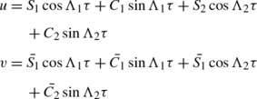
The general solutions for pure imaginary roots are given (Szebehely 1967a, 1967b)

where S i , \(\bar{S_{i}}\), C i and \(\bar{C_{i}}\) (i=1,2) are constants.
Hence, the collinear point L 2κ is stable in this case.
The coefficients of \(S_{1},C_{1},\bar{S_{1}}\) and \(\bar{C_{1}}\) of the frequency σ 1 are called the long period terms, while the terms \(S_{2},C_{2},\bar{S_{2}}\) and \(\bar{C_{2}}\) associated with the frequency σ 2 are the short terms; where the frequencies are given by

where δ=κ(1+2f 2κ )≪1.
Now, finding first and second derivatives of (46), substituting them in the first two equations of (40); separating and equating the coefficients and solving simultaneously, we get

where
Substituting (14), α 2=1+2ϵ, β=1+ϵ′ and the partial derivatives (42) in the above, yields

where
Setting the short periodic terms equal to zero and substituting τ=0, with initial conditions in (45), we get
Numerically, we properly select initial conditions just to the right, and a little below the collinear points L 2κ , when ϵ′=0 and ϵ′=0.003 respectively:
Using the first equation of (46), (48) and (49) in (47) for i=1, yields

Similarly, the coefficients of the short period terms are:

Equations (49) and (50) give the value for the coefficients of the long period terms, while the coefficients of the short period terms are given by system (51). These give the values of the long and short period terms at which the collinear points L 2κ is stable.
Any case, different from case 1 above, results in a solution of the type

Here, A j′s and B j′s (j=1,2,3,4) are constants and all λ i , i=1,2,3,4 are real.
In this case, the collinear point L 2κ is unstable due to the presence of exponential functions and a positive root. Therefore, the collinear point is stable or unstable due to κ, a constant of the Gylden-Meshcherskii problem, small perturbations given in the Coriolis and centrifugal forces, radiation pressure, oblateness term and the mass parameter. The same stability analysis may be followed in case of L 1 and L 3.
4.2 Triangular points
The characteristic equation in the case of triangular point is obtained by putting ζ=0 in the variational (40), to get

In this case, we have:

here \(N=4\kappa^{\frac{2}{3}-(\beta+\kappa-1)^{\frac{2}{3}}}\).
In the computation of the above derivatives, we have neglected second and higher order terms of α 1, 1−q 2 and their product as they are considered very small. Factorizing and ignoring product of β−1, with α 1 and 1−q 2 in the above partial derivatives yield:

The characteristic equation in the case of triangular point is obtained by putting ζ=0 in the variational equation (40), with the substitution of (53) and (14), and ignoring product and higher order terms of very small quantities, to get
where
are the roots of (54), and D=P 2−4Q,


The discriminant D of (54) is given by,

Now, D is a monotonous function of ν in the interval (\(0,\frac{1}{2}\)) and has values of opposite signs at endpoints for some range of κ. So there are different values of ν, say \(\nu_{C_{\kappa}}\) in this range at which the discriminant vanishes and are:
where

\(\nu_{C_{\kappa}}\) are the critical mass parameter which exist for different values of κ (see Fig. 3), and describes the joint effect of the involved parameters. Though, κ can take values above β−1 and below infinity. However, we consider only values in the range 0.71459<κ≤9.952135, for values of κ outside this interval do not result to physically meaningful critical mass parameters as they turn out to be either negative or indeterminate quantities.

Graph of κ and the critical mass parameters \(\nu_{C_{\kappa}}\)
The critical mass values \(\nu_{C_{\kappa}}\), for values of kappa in this interval are:


Table 2 gives the numerical computations of \(\nu_{C_{\kappa}}\) and \(\nu_{0_{\kappa}}\) for κ in the interval [0.7145311,9.952136] for, q 2=0.9985, α 1=0.02, α=1.001, β=1.002.
We observe that for 0.7145311≤κ<0.71459 and κ>9.952135 with the allowance for oblateness of the first primary, \(\nu_{C_{\kappa}}\) is either complex or negative; therefore the physically possible range of κ is 0.71459≤κ≤9.952135. However, in the absence of oblateness, i.e., α 1=0, the range becomes 0.7145311<κ≤9.9521. For example when κ=0.7145312, we get \(\nu_{C_{\kappa}}=-14.5207\) which is unrealistic; however when the first primary is spherical, the critical mass parameter becomes \(\nu_{C_{\kappa}}=1.28339\). Below is a graphical representation of \(\nu_{C_{\kappa}}\) as a function of κ in the interval 0.71459≤κ<9.952136 for, q 2=0.9985, α 1=0.02, α=1.001, β=1.002.
Now, since the nature of the characteristic roots (54) depend on the nature of the discriminant, small perturbations, mass ratio, oblateness and the constant κ, we consider the three regions of the discriminant D coupled with the changes in P, which is due to κ, ν, α 1 and whether 8ϵ−3ϵ′<=>0.
-
1.
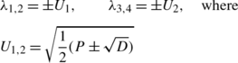
A condition for pure imaginary roots of (54) is that simultaneously \(0<\nu<\nu_{C_{\kappa}}\), D>0 and P>0, and are represented as:
$$\lambda_{1,2,3,4}=\pm i\Lambda_n\quad (n=1,2)$$where
$$\Lambda_{1,2}=\sqrt{\frac{1}{2}(-P\pm\sqrt{D})}$$In this case the triangular point is stable.
The general solution can be written (Szebehely 1967a, 1967b) as
 (59)
(59)where, S i , \(\bar{S_{i}}\), C i and \(\bar{C_{i}}\) (i=1,2) are constants.
-
2.
For \(0<\nu<\nu_{C_{\kappa}}\), D>0 and P<0. In this case the roots are real and distinct and can be written as
The general solution for real roots with the condition P<0 is represented as
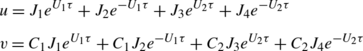 (60)
(60)where C 1, C 2, J 1 and J 2 are constants. A positive root induces instability at the triangular point.
-
3.
When \(\nu_{C_{\kappa}}<\nu\leq\frac{1}{2}\), D<0 and P<0, \(0<P<2\sqrt{Q}\). The real parts of two of the values of λ are positive and equal. Therefore, the triangular point is unstable.
-
4.
When \(\nu=\nu_{C_{\kappa}}\), D=0. The following cases are possible.
-
(i)
If P<0, two roots are real and equal, while the other two are negative and also equal. In this case, the triangular point is unstable.
-
(ii)
If P=0, here all the roots are zero, and the triangular point is unstable.
-
(iii)
If P>0, all four roots are imaginary, in which two are positive and equal and the other two are negative and equal. In this case we have the resonance case of second order. Here, since the frequencies are equal and of same sign, the equilibrium point is stable (Gozdziewski 2003).
Hence, we conclude that the triangular point of the autonomized system is stable or unstable for \(0<\nu\leq\nu_{C_{\kappa}}\) and unstable for \(\nu_{C_{\kappa}}<\nu\leq\frac{1}{2}\), depending on the choice of the arbitrary constant κ, the mass ratio, oblateness coefficients and whether the points (ϵ,ϵ′) lies in one or the other of the two regions in which the (ϵ,ϵ′) plane is divided by the line 8ϵ−3ϵ′=0.
-
(i)


4.3 Out of plane points
We consider the stability of the out of plane point L 6, that of L 7 can be analogously obtained. The characteristic equation corresponding to the variational equation (40), in the case of the out of plane points is:

where


These derivatives have been evaluated at the out-of-plane equilibrium points and we have neglected second and higher order terms and product of α 1 with 1−q 2 and β−1=ϵ′.
Now, substituting (62)–(66) and (14) in (61), results in
where

with

The stability of the out of plane points L 6 is determined by the roots of the characteristic equation (67). We perform a numerical exploration to compute the out of plane points, the partial derivatives and values of the quantities p, q and r using the software package Mathematica (Wolfram 2003) for values of κ>1, q 2=0.9855, α=1.001, β=1.002, α 1=0.02 and found that the signs of the quantities p, q and r could be negative or positive depending on the interval where κ lies. The following cases have been considered:
-
(i)
p<0, q>0 and r<0, there is one change in sign, which implies there is exactly one positive root according to the Descartes rule of sign.
-
(ii)
p>0, q<0 and r<0, there is also one change in sign.
-
(iii)
p>0, q<0 and r>0, there are two changes in sign indicating there two positive, two negative and two imaginary roots
The stability of the out of plane points would have been achieved if a fourth case, that is p<0, q>0 and r>0. However, since this case does not arise, as there is at least a positive root in each of the cases above, we conclude that the out of plane points of the autonomized dynamical system are in general an unstable equilibrium points only due to the positive roots.
5 Stability of equilibrium points of the non-autonomous system
The analysis of the stability of the particular solutions L i (i=1,2,…,7) would depend on the methods applied, since these equilibrium points are themselves time dependent. For example, using the definition of a Lyapunov stable solution (Krasnov et al. 1983), we have in the triangular case:
Equation (69) proves the instability of the solutions x(t) and similarly for y(t), according to the Lyapunov’s theorem, and is same as the result of Luk’yanov (1990).
The relationship between the old and new independent variables t and τ are given (Poincare 1911; Singh and Leke 2010) as
and
where
Equation (70) implies that as t is approaching ∞, τ is also always approaching a finite value, while (71) indicates that \(\lim_{t\rightarrow\infty}\frac{\tau}{t}\) always tends to a positive finite value Γ. However, this finite values decreases due to oblateness of the first primary.
The system (15) of equations with constant coefficients and the reducible system are regular. The system (7) with variable coefficients is reducible due to the Meshcherskii transformation (8). Therefore, we apply Lyapunov’s theorem, using the Lyapunov Characteristic Numbers (LCN) on the stability of the motion around the equilibrium solutions of the system (7). The calculations of the Lyapunov characteristic numbers here are limited to finding the maximum LCN, which gives a computed value that we use as a metric to give a qualitative indication of how stability vary over the solutions. Following Singh and Leke (2010), the LCN of the triangular solutions varying with time with the consideration that as t→∞, τ is approaching a finite value, is:
similarly,
Thus, the Lyapunov characteristic number is zero for triangular solutions, therefore the stability or instability of the perturbed motion cannot be determined directly from the triangular solutions.
Using (39), the particular solutions of the system of equations with variable coefficients (7) can be represented (Singh and Leke 2010), with given solutions (59) and transformation (8) as:

where ξ 0, η 0 are coordinates of the test particle.
These solutions correspond to the region where \(0<\nu<\nu_{C_{\kappa}}\), P>0. Numerically, this holds when 0.002<κ<1.31169451; when there are no small perturbations in the Coriolis and centrifugal forces, we have 0<κ<1.311. Further, if the first primary is not an oblate spheroid, then we have \(0<\kappa<\frac{4}{3}\), and agree with Singh and Leke (2010).
Similarly, the particular solutions with conditions \(0<\nu<\nu_{C_{\kappa}}\), P<0 using (39), solutions (60) and transformation (8) can be represented as:

The solutions (74) correspond to the region where, P<0. This region is determined by the parameter κ, oblateness of the first primary and whether 8ϵ−3ϵ′<=>0; since in both cases \(0<\nu<\nu_{C_{\kappa}}\) (D>0).
For the solutions (66), their LCN’s are (Singh and Leke 2010)
In view of the particular solutions (74) and using (71); their LCN’s are:
Similarly
Therefore, the LCN are negative for solutions with positive exponents, positive for solutions with negative exponents, and, zero for solutions with imaginary exponents and constant solutions. Hence, when the roots of characteristic equation of the autonomized equations are positive, then the LCN of the solutions varying with time is negative, and consequently the solutions are unstable according to the Lyapunov theorem. If these roots are pure imaginary quantities, then the LCN of corresponding solution varying with time is zero; in this case the stability or instability of the solutions cannot be determined. Finally, when the roots are negative, the LCN of corresponding time-dependent solutions is positive and consequently stable.
The same stability analysis can be done in the case of the collinear and out-of-plane solutions of the non-autonomous system.
6 Discussions and conclusions
The system (7) of equations of motion is unlike those obtained by Luk’yanov (1990) due to the presence of radiation of the second primary, oblateness coefficient of the first primary and small perturbations in the Coriolis and centrifugal forces. We observe that the perturbation given in the centrifugal force which is considered so small permits the appearance of κ in the collinear and triangular equilibrium points. The positions of these points are different from those of Singh and Leke (2010) and Singh et al. (2010).
The characteristic equation (43) of the collinear equilibrium points is different from those of Singh and Leke (2010) due to the oblateness of the first primary. It is seen that the coefficients can take either positive or negative values because of the presence of the arbitrary constant which takes values between zero and infinity, and the other parameter involved. Consequently, a stable collinear point is possible under some conditions.
Equation (55) represents the combined actions of the involved parameters on the critical mass ratio. If in (55), we annul the effect of the small perturbations and radiation pressure and oblateness of the first primary (i.e. ϵ=ϵ′=0, q 2=1, α 1=0) and κ=1,2; then \(\nu_{C_{1,2}}=\nu_{0_{1,2}}=0.038520\), this fully coincide with the Routhian value (Szebehely 1967a, 1967b). We observe from system (56) that, for \(0.7145312\leq\kappa<\frac{4}{3}\) the Coriolis force has a stabilizing tendency while the centrifugal force, radiations pressure and oblateness of the first primary have destabilizing behaviors in this range of κ. When \(\kappa=\frac{4}{3}\), all these parameters are annulled and have no effect (see (57)). For \(\frac{4}{3}<\kappa\leq9.952135\) the Coriolis force and the radiation pressure of the second primary remains all through a destabilizing parameter, while here, the oblateness of the first primary assumes the role of a stabilizing parameter. The small perturbation in the centrifugal force plays a stabilizing role only when \(\frac{4}{3}<\kappa\leq7\) and is destabilizing outside this range of kappa; while for \(\frac{4}{3}<\kappa\leq5\) oblateness of the second primary has a destabilizing tendencies which afterwards becomes stabilizing for 6≤κ≤9.952135. Hence the stabilizing or destabilizing behaviors of the Coriolis & centrifugal forces and oblateness is controlled by kappa. It is seen that (except for the case when \(\kappa=\frac{4}{3}\)), the radiation pressure always has a destabilizing tendency. This behavior gets weaker with increase in kappa in the interval \(0.7145312\leq\kappa<\frac{4}{3}\); and has no effect for \(\kappa=\frac{4}{3}\) and interestingly grows stronger for \(\frac{4}{3}<\kappa\leq9.952135\). Our numerical computation reveals that for any |ϵ|≪1, |ϵ′|≪1, 1−q 2≪1 and \(0.71460\leq\kappa<\frac{4}{3}\), every \(\nu_{C_{\kappa}}<\nu_{0_{\kappa}}\); consequently the region of stability is decreasing. This is so because of the inclusion of oblateness of the first primary. If this is ignored i.e., the first primary is spherical, we’ll have \(\nu_{C_{\kappa}}>\nu_{0_{\kappa}}\) which implies that the region of stability is increasing. When \(\kappa=\frac{4}{3}\), it coincides and equal zero; while for \(\frac{4}{3}<\kappa\leq9.952135\), due to oblateness every \(\nu_{C_{\kappa}}>\nu_{0_{\kappa}}\), which implies that the region of stability of the triangular point is increasing. If α 1=0, the reverse is the case as in Singh et al. (2010). The results of Szebehely (1967b), SubbaRao and Sharma (1975), Bhatnagar and Hallan (1978), Bekov (1988) and Singh et al. (2010) can be confirmed here from our results.
Our results show that a condition for stable triangular points is when the mass ratio is in the region \(0<\nu<\nu_{C_{\kappa}}\) and P>0. Numerically we must have 0.002<κ<1.31169451. If 8ϵ−3ϵ′=0, α 1=0 then \(0<\kappa<\frac{4}{3}\) and agrees with Singh and Leke (2010).
We conclude that the stability behavior of the collinear of the restricted three body problem with constant masses which always remain unstable changes here to a stable equilibrium point due to κ. However, the behavior of the out-of-plane equilibrium points remain unstable despites the introduction of a small perturbation in the centrifugal force, radiation pressure, oblateness of the first primary and κ.
The triangular points are stable under some conditions; in this case, the decrease, increase or non existence of the region of stability of the triangular points depends on the arbitrary constant κ and oblateness α 1 of the first primary and the signs of the small perturbations. The overall effect of these parameters is that the region of the stable motion increases.
For the stability of the equilibrium points varying with time, we conclude that, the introduction of oblateness of the first primary does not change the stability analysis of any of the equilibrium solutions of system (7). Hence, they remained unstable.
References
Bekov, A.A.: Sov. Astron. 32, 106 (1988)
Bekov, A.A., Beysekov, A.N., Aldibaeva, L.T.: Astron & Astrophys. Trans. 24, 311 (2005)
Bhatnagar, K.B., Hallan, P.P.: Celest. Mech. 18, 105 (1978)
Gelf’gat, B.E.: Modern Problems of Celestial Mechanics and Astrodynamics, p. 7. Nauka, Moscow (1973)
Gozdziewski, K.: Celest. Mech. Dyn. Astron. 85, 79 (2003)
Gylden, H.: Astron. Nachr. 109, 1 (1884)
Helhl, F.W., Kiefer, C., Metzler, R.J.K.: Theory and Observation. Springer, Berlin (1998)
Krasnov, M.L., Kiselyov, A.I., Makarenko, G.I.: A Book of Problems in Ordinary Differential Equations, pp. 255–291. Mir, Moscow (1983)
Lopez, G., Barrera, L.A., Garibo, Y., Hernandez, H., Salazar, J.C., Vargas, C.A.: Int. J. Theor. Phys. 43, 10 (2004)
Luk’yanov, L.G.: Sov. Astron. 33, 92 (1989)
Luk’yanov, L.G.: Astron. Zh 67, 167 (1990) (Sov. Astron. 34, 1)
Meshcherskii, I.V.: Astron. Nachr. 159, 229 (1902)
Meshcherskii, I.V.: Works on the Mechanics of Bodies of Variable Mass (in Russian), p. 205. GITTL, Moscow (1952)
Nuth III, J.A., Hill, H.G.M., Kletetschka, G.: Nature 406, 275 (2000)
Poincare, H.: 1911 Leçons sur les Hypothesis Cosmogoniques
Singh, J., Leke, O.: Astrophys. Space Sci. 326, 305 (2010)
Singh, J., Leke, O., Umar, A.: Astrophys. Space Sci. 327, 299 (2010)
Sommerfeld, A.: Lectures on Theoretical Physics, vol. 1. Academic Press, San Diego (1964)
SubbaRao, P.V., Sharma, R.K.: Astron. Astrophys. 43, 381 (1975)
Szebehely, V.G.: Theory of Orbits. Academic Press, New York (1967a)
Szebehely, V.G.: Astron. J. 72, 7 (1967b)
Wolfram, S.: The Mathematica Book, 5th edn. Wolfram Media, Champaign (2003)
Author information
Authors and Affiliations
Corresponding author
Rights and permissions
About this article
Cite this article
Singh, J., Leke, O. Equilibrium points and stability in the restricted three-body problem with oblateness and variable masses. Astrophys Space Sci 340, 27–41 (2012). https://doi.org/10.1007/s10509-012-1029-2
Received:
Accepted:
Published:
Issue Date:
DOI: https://doi.org/10.1007/s10509-012-1029-2