
Abstract
The item-based collaborative filtering technique recommends an item to the user from the rating of k-nearest items. Generally, a random value of k is considered to find nearest neighbor from item-item similarity matrix. However, consideration of a random value for k intuitively is not a rational approach, as different items may have different value of k nearest neighbor. Sparsity in the data set is another challenge in collaborative filtering, as number of co-rated items’ may be few or zero. Due to the above two reasons, collaborative filtering provides inaccurate recommendations, because the predicted rating may tend towards the Mean. The objective of the proposed work is to improve the accuracy by mitigating the above issues. Instead of using a random value of k, we use the most similar neighbor for each target item so as to predict the target item, since finding k for different target item is computationally expensive. Bhattacharyya Coefficient is used as a similarity measure to handle sparsity in the dataset. The performance of the proposed algorithm is tested the datasets of MovieLens and Film Trust, and experimental results reveal better prediction accuracy than the best of the prevalent prediction approaches exist in literature.
1 Introduction
With the improved technology of the internet based applications, the most influential method of marketing, promoting and advertising is the internet itself. Recent commercial and entertainment websites are implementing various recommendation algorithms which help in persuading the users to think about the offer that the website promotes for a product. Collaborative Filtering (CF) is an approach to perform predictions based on similar users or items. There is a growing interest of CF techniques in the research community because of the following reasons: i) It benefits from large user bases, ii) It’s flexible across different domains, iii) It produces more serendipitous recommendations, and iv) It can capture more nuances around items. Model-based and memory-based CF are the two widely used algorithms of CF-based recommender system (RS). The main advantages of model-based CF are scalability and prediction speed, but it suffers from the issues of inflexibility, and Quality of predictions [1]. Memory-based CF is one of the simplest forms of CFs used in many early commercial applications. The effectiveness and ease of implementation of memory-based CF may still attract more and more attention of the modern research community, in spite of the approach being a relatively old one [2]. Memory-based CF has better scope for successful recommendation because it can sustain on a very little data feed. For instance, the user’s rating about an item is enough for performing analysis and easy adjustment of new data; independent of content of the items being recommended and good correlation with similar items [3, 4]. The two algorithms used in memory-based CF are user-based CF and item-based CF. User-based CF employs the similarity between the target user and other users, whereas item-based CF uses similarity between the target item and other items. The underlying assumption of the user-based CF approach is that if a person ‘A’ has the same opinion as a person ‘B’ on an issue, ‘A’ is more likely to have B’s opinion on a different issue than that of a randomly chosen person [5]. Items-based CF launched by Amazon has been widely adopted across all the web giants because of the following reasons [6,7,8,9,10]: (i) User-based CF is computationally expensive as the entire system model has to be recomputed because user profiles changes quickly. (ii) improved scalability and prediction accuracy. (iii) This method is a more stable method than user-based CF in sparse dataset because the average item has a lot more ratings than the average user and as a result individual ratings doesn’t impact much.
Item-based CF relies on the ratings of k nearest neighbors to predict the rating of target item. A random value of k is considered and is fixed for different target items. Besides this, sparsity is another issue in the context of prediction accuracy because in the presence of sparsity the number of co-rated items’ is reduced to few or zero. Owing to the above mentioned reasons, the weighted sum of the k nearest neighbors’ rating may result in incorrect prediction, which in turn degrades the accuracy of the item-based CF. Moreover, we have observed that predicted rating in such situations leans towards the mean.
However, in real life different people may have different number of nearest friend and the same analogy can be used to find k nearest neighbors in rating prediction for target item in item-based CF. Moreover, correlation based similarity measure is not suitable in sparse dataset [11].
Although people may be benefited from item-based CF, an obvious question is: should we use strategies that adopted the weighted sum of the rating of k nearest neighbors or we should find the optimal value of k for different target item? or is it better to rely on the rating of ‘most’ similar item for recommending a target item?
This paper proposes a modified prediction approach to improve the accuracy of item-based CF. We consider Bhattacharyya Coefficient (BC) as a similarity measure (SM), and only a single item that is ‘most’ similar to the ‘item-to-be-recommended’ to the target user. Our contributions of this paper are as follows:
-
A modified prediction approach is proposed for the item-based CF. In modified prediction approach Bhattacharyya Coefficient is used in SM to increase the proportion of similar items, and ‘most’ similar item is considered for rating prediction because number of k most similar items are different for different target items.
-
A comparison has been adopted to select the best prediction approach from the traditional prediction approaches.
-
The proposed prediction approach is compared with the existing best prediction approach in item-based collaborative filtering. The experimental results have been shown on the MovieLens and Film Trust datasets in Section 5, where the proposed approach provides the enhanced accuracy.
Rest of the paper is structured as follows. Section 2 discusses the Background and Related Work. Motivations, the proposed approach and algorithm are portrayed by Sections 3 and 4, followed by the Experimental Analysis and Results. The last section concludes our paper with future direction.
2 Background and related work
The goal of CF is to inform the user about new items or recommend the certain items based on the user’s need. The memory-based CF is also called as neighborhood-based CF. The framework of memory-based CF can be broadly classified into the following parts [8] as illustrated in Fig. 1: 1). Data Collection, 2). Data Processing using Similarity Metrics, 3) Rating Prediction, and 4) Top-N Recommendation. The first part of the framework consists of the collection of rating information from users. The collected rating information is used to determine the k most similar items of the target item using different similarity measures. After that, calculated k most similar items of the target item are used to predict the missing rating of the target item. And, based on these predicted ratings a list of Top-N items is generated and recommended to the target user.

Conceptual framework of memory-based Collaborative Filtering
2.1 Data collection
Data Collection is the lifeblood of RS. Explicit and implict are the two rating collection methods used in the memory-based CF [12]. In a traditional memory-based CF scenario, there is a list of m users, i.e. (U={u1, u2,.......,um}) and a list of n items, i.e. (I={i1, i2,.......,in}). Each user has a list of items about which the user expresses his opinion explicitly using rating score within a certain numerical scale. In implicit way, the system tries to extract the user’s preferences based on their behaviour, i.e. 1) Time spent in searching an item; 2) Click behaviour; and 3) Movement of mouse cursor. Finally, user-item rating dataset is generated by combining the above mentioned methods.
2.2 Data processing using similarity metric
In memory-based CF approach, the similarity between a pair of items is calculated using the SM as listed in the Table 1.
2.3 Rating prediction
Rating prediction for the target item i of active user u is determined by a set s of similar items corresponds to item i. The ratings in item set s which are already given by user u are used to predict whether the user will like the item i or not. Different techniques of weighted sum such as Mean Centering (MC), Weighted Average (WA), and Z-Score (ZS) have been used for prediction computation. They use rating of similar items as a weighting factor. The details of these prevalent prediction approaches (PAs) are as follows:
- Mean Centering: :
-
It is the most prevalent PA [17] of item-based CF. The equation to predict the rating is shown below.
$$ \hat{r_{ui}} = \bar{r_{i}} + \frac{{\sum}_{j \in N_{u}(i)} sim(i,j)(r_{ju} - \bar{r_{j}})}{{\sum}_{j \in N_{u}(i)} |sim(i,j)|} $$(1)Here, \(\hat {r_{ui}}\) represents the predicted value of item i of user u.
- Weighted Average: :
-
The weighted average approach predicts the rating for an unrated item using the correlation values as weights [7]. The equation to predict a rating is given as follows:
$$ \hat{r_{ui}} = \frac{{\sum}_{j \in N_{u}(i)}sim(i,j)r_{ju}}{{\sum}_{j \in N_{u}(i)}|sim(i,j)|} $$(2) - Z-Score: :
-
This approach was initially proposed to calculate the financial risks (such as to calculate the bankruptcy of a bank). Unlike Mean Centering, the standard deviation of ratings of the item is also taken into consideration [18, 19]. The equation of Z-Score is as follows:
$$ \hat{r_{ui}} = \bar{r_{i}} + \sigma_{i}\frac{{\sum}_{j \in N_{u}(i)} sim(i,j)(r_{ju} - \bar{r_{j}})/\sigma_{j}}{{\sum}_{j \in N_{u}(i)} |sim(i,j)|} $$(3)Here, σi and σj are the standard deviation of rating of item i & j respectively. Some references of frequently used PAs in item-based CF are shown in Table 2.
2.4 Top-N recommendation
The predicted ratings are fed to the RS, which generates a user specified list, called Top-N recommendation [35]. The ratings in the form of user-item dataset are inherently sparse in the real world. For example if a user rates 1% of the 2 million items available on an e-commerce website, he/she may only rate at most 20,000 items [7] which causes the dataset to become sparse.
There exists a plethora of works to improve the accuracy of the user and item-based CF in literature. The descriptions of some of the most relevant literature are as follows:
2.4.1 User-based CF
Bobadilla et al. [39] have analyzed the dataset of Movielens, Netflix, and FilmAffinity, and suggested that traditional similarity metrics can be improved by appending contextual information of users. According to their hypothesis, the similarity value must be modulated by the singularity value, in such a way that the singular similarity should be awarded a higher value than any normal similarity. Singularity gives excellent results for prediction in user-based CF.
Liu et. al have proposed a novel similarity metric based on the combined information entropy with compressive distance weight based on the probability distribution of rating distance [40].
Ai et. al have introduced a network model to evaluate the similarity of the items using a number of corresponding reviews given by a user and differences between those viewpoints. The calculated similarity is compared with Pearson approach [29].
Cacheda et al. [41] have deliberated two new metrics to measure the precision on items and the results have revealed the weaknesses of many algorithms in extracting information from user profiles under sparsity conditions. An alternative approach has been presented based on the interpretation of the tendencies or differences between users and items. Two new metrics, i.e. Good Items MAE (GIM), and Good Predicted Items MAE (GPIM), are used to measure the quality of a recommendation list using prediction accuracy techniques. The online datasets have been used to simplify the evaluation and also used at the same time, in the detection of undesirable biases in the predictions. Furthermore, a novel strategy of memory-based CF has been proposed based on the tendencies or differences between users and items, instead of their similarities.
Bilge et al. [42] have compared traditional approaches with multi-dimensional distance to determine appropriate neighbors which produce more accurate recommendations by utilizing multi-criteria item-based CF algorithm instead of a single criterion rating-based algorithm. Giving rating on various criteria of an item becomes boring to a user, and it tends to a huge sparse dataset.
Hui et al. [43] have introduced a theoretical framework to improve the item-based collaborative Filtering using TAG similarity to minimize the sparsity and cold start issue. However, the performance of the proposed system is not tested using any real dataset. To mitigate the problem of scalability and sparsity, a clustering method is suggested by Wen et al. [44] to improve the performance of item-based CF when the item size is large. The authors [4] have presented a new user similarity model to improve the recommendation performance when only a few ratings are available. The model not only considered the local context information, i.e user ratings but also the global preference, i.e. proportion of common ratings of the user. They also analyzed the disadvantages of the existing similarity measures. Finding similar neighbors with the help of global preferences of a user is not suitable in highly sparse dataset.
Koohi and Kiani have explored a method of enhancing the performance of the recommendation systems by utilizing the subspace clustering methods to derive the best similar neighbors without any varying parameters [45]. The aforesaid user lists are used to construct a tree, where the target item is the root and the similar items are its children and so forth. The similarity of the target item is calculated with correlation to its multiple children and then fed to a prediction approach for rating prediction.
Ye and Zhang have introduced a similarity paradigm that evaluates user similarities by utilizing the user’s interest based on certain predefined categories and the item similarities are detected using association rule mining [46]. The similarities are then used to predict the ratings using rating prediction approach.
Patra et al. [11] have introduced a new similarity measure based on Bhattacharyya coefficient to improve the accuracy of CF due to the sparsity. Suryakant and Mahara have proposed a novel similarity mechanism to accurately detect the correlation among the users by evaluating the mean divergence of their habits upon the rated items [47]. The correlation values are used to predict the ratings of target items.
Stephen et al. have addressed the issues of data sparsity for evaluation of the similarity in memory-based CF [27]. They have provided a comprehensive study of similarity metrics and proposed a method that categorizes the items in a hierarchical order that helps in reducing the sparsity of user-item rating dataset. To increase the accuracy of user-based CF, the average rating of users has been taken as an additional argument in Jaccard based similarity measure by Ayub et al. [48].
In spite of the improved similarity measure, prediction score algorithms also play a significant role in the accuracy of memory-based CF. To justify the aforesaid statement, Al-bashir et al. have introduced the TOPSIS technique [49]. In this paper, conventional prediction approaches are replaced by TOPSIS technique to obtain improved recommendations. TOPSIS technique utilizes the similarity value of Top-N users and multi-attribute decision-making (MADM) technique to generate the Top-N recommendations for the target user. However, we observed that the most of the papers available in the literature attempts to improve the accuracy of user-based CF by proposing a new similarity measure algorithm. All of them use aggregation to predict the rating of the target user.
2.4.2 Item-based CF
As per our knowledge, very few works have been addressed towards the enhancement of accuracy in item-based CF. One of the major issues of traditional similarity measures is that equal weight is assigned to all items in the computation of item-item similarity. An item which is recently rated by a user should have higher preference than the previously rated item by that user. To consider user purchase behavior on time, Ding et al. have introduced a time function to compute the similarity between two items [50]. With the help of time function, the proposed algorithm assigns time weights to different items in decreasing order from recent to old. In this direction, Zhang et al. have applied a time-aware similarity computation to improve the performance of item-based CF [51]. In their proposed approach, the items which are more relevant to the target users have assigned with higher weights. Gao et al. have presented a PageRank-based ranking approach to incorporate the weighted user-rank in the calculation of item-item similarity [52].
Diversity is considered as a desirable property of a good RS. An accurate RS may have a diverse recommendation list for each target user. In this direction, Jain et al. have introduced a multi-objective recommender framework to recommend diverse and novel items [53]. The proposed framework adopts a similarity model using Bhattacharyya Coefficient to compute the nearest neighbors, and a random value of k nearest neighbors to evaluate unknown ratings.
We can observe that the most of the existing work of memory-based CF has hinged around the combination of an improved similarity measure and the traditional prediction approach to improve the recommendation accuracy as shown in Table 3.
Research article available in the literature to improve the accuracy of CF in sparse dataset mainly focuses on finding new techniques for similarity measure. However, the size of nearest neighbor in prediction computation can profoundly affect the performance of item-based CF in sparse dataset. Proper selection of optimum number of nearest neighbor for rating prediction can significantly improve the performance of CF.
3 Motivation
Prediction accuracy in traditional PAs adversely affected when the dataset is sparse and users’ ratings are few or no co-rated. The following two datasets with different sparsity levels are used to explain the limitation of traditional PAs. Table 4 represents a user-item rating dataset with moderate sparsity, whereas Table 5 is contained relatively high sparsity. The symbol ‘?’ in the dataset, indicates the user does not rate the particular item.
To find the nature of traditional PAs in item-based CF, we remove randomly 5% and 10% given ratings from Tables 4 and 5, and predict these removed ratings. Figure 2 illustrates the accuracy of PAs using different threshold values of k in most similar items. The equation for computing mean absolute error (MAE) is as follows:
Where, \(<p_{i}, \hat {q_{i}}>\) represents the ratings-prediction pair and N denotes the total number of ratings-prediction pair.

Prediction accuracy using different number of similar items at various sparse datasets
The above graph clearly depicts the fact that prediction error using all PAs significantly increases when the sparsity of dataset is increased from 5% to 10%. In most of the cases, we can also notice that prediction error increases for the higher value of k in most similar items, and for k= 1 (‘most’ similar item) minimum error is achieved. The obvious reason is that when sparsity of the dataset and prediction error are increased the standard deviation (SD) becomes very less, as a result, the predicted rating leans towards the item’s mean rating.
The observations (Figs. 2 to 3) clearly explain the relationship between prediction accuracy and SD. The SD of the variable can be calculated by following:
where xi is the predicted value of item i, μ is the mean of item i, and N is the total number of observation.

Standard Deviation of items’ rating at various sparse datasets
From Figs. 2 to 3, we can notice that prediction error is directly proportional to the sparsity of the dataset, whereas in most of the cases, for a large value of k, the prediction error and average SD of items are high, i.e. more the SD less will be the prediction error. The above
observations reveal the fact that for a large value of k in a sparse dataset, the recommended item will reflect the average view, which deviates from the basic objective of collaborative filtering. In such scenario, to provide personalized recommendation in a sparse dataset, it is necessary to reduce the number of similar items in rating prediction.
4 The proposed approach
The input of the proposed approach is a user-item dataset generated from the tuple < Uid, Iid, Rating >, where Uid represents the set of unique user, Iid denotes the set of unique item and Rating identifies the user’s feedback on the particular item. The prediction of missing/unknown ratings play a vital role in CF based recommendation systems, as low accuracy may cause the enterprise to lose many potential customers. Many top brands like Amazon, Netfix, and MovieLens etc. investing a large portion of their budget to improve the accuracy of CF-based RS [7, 54, 55] to get competitive advantage. In this direction, we propose the system model as shown in Fig. 4.

Rating based movie recommender system
4.1 User review model
The review model consists of the user set (Uid) of size m and item set (Iid) of size n, represented as a m×n rating matrix. For a given user-item rating dataset, the target items represented as: ∃j∀i¬R(i,j)→ T(i,j), which indicates, item j will be the target item for user i, if he/she has not rated it.
4.2 Finding the ‘Most’ similar item using similarity measure using Bhattacharyya Coefficient
The proposed approach uses the rating of the ‘most’ similar item corresponding to the target item. For each item i, the ‘most’ similar item j is represented as: ∀i∃!j (S(i,j) ∧ max(Simj) → SM(i,j), where S(i,j) denotes the similarity value of item i and item j computed using BC and SM(i,j) means that the similarity value between item i and j is found to be maximum.
4.3 Rating prediction model
The Top-N recommendation list includes only those items whose predicted rating satisfies system specified threshold value. Rating prediction of target item i in the proposed model is formulated as: RT(i,j) = SM(j,k)*R(i,k), where RT(i,j) shows the rating value of user i on target item j, SM(j,k) represents that k is the ‘most’ similar item of j and R(i,k) denotes the rating of user i on item k.
If multiplication of SM(j,k) * R(i,k) is ≤ 0 then RT(i,j) = RA(j), where RA(j) stands for average rating of item j.
4.3.1 Proposed algorithm
Determining similarity between items is crucial as all neighbors’ ratings may not be equally valuable [56]. Two items are said to be similar if their rating patterns are same. With this approach, the missing rating is predicted using similarity value and rating information of the ‘most’ similar item. Hence, prediction formula of Congenerous items using Congenerous Rating (CR) becomes:
Where, \(\hat {r_{ui}}\) represents the predicted rating of item i of user u. sim(i,j) means that item i and j are found to be ‘most’ similar, and ruj is the available rating of item j given by user u. Table 6 shows the mathematical notations used in the proposed approach, and the detail steps are shown in Algorithm 1.

The suggested algorithm can be partitioned into three sections. These sections are the elimination of self-similarity, sorting of item similarity values for n items, and rating prediction. Table 7 illustrates the time/running complexity of the proposed algorithm in different cases.
5 Experimental analysis and results
The effectiveness of the proposed approach is explained in this section. The performance of the proposed method is compared with the best PA available in the literature. The following two steps are used to perform the analysis.
-
1.
Selection of the best prediction approach.
-
2.
Comparison of the existing best prediction approach and the proposed prediction approach.
5.1 Selection of the best prediction approach
For evaluating the accuracy of the three traditional PAs available in the literature, their relative performances are compared using BC. Further, the PA that excels among the three is compared against the proposed prediction approach in order to reach the final conclusion. The datasets that are usually generated from MovieLens and other such open sources suffer from a great deal of sparsity and ranges from being moderately sparse to highly sparse. The standard datasets of MovieLens, viz., ml-20m, ml-100k, and ml-1m, and Film Trust used in the experimental analysis are highly sparse. Brief details of these four datasets are shown in Table 8.
In order to check the effectiveness of the proposed approach in different levels of sparsity, the dataset ml-20m is modified into dataset 1* having lesser sparsity. The dataset 2, dataset 3, and dataset 4 are used without any modification. Thus, the modified ‘dataset 1*’ becomes moderately sparse based on the following conditions:
-
1.
Only those users who rated at least 100 movies within the dataset.
-
2.
Only those movies that were rated by at least 1000 different users.
Hence the details of the modified dataset 1* and other three datasets (dataset 2, dataset 3, and dataset 4) used in the experimental analysis is shown in Table 9.
The analysis reveals that at 5%, 10%, and 15% sparsity, the MC approach comes out with the best results. We create, sparse datasets by randomly removing 5%, 10%, and 15% of given ratings from datasets. All positive item similarity value have been considered in this comparative results. Though there is an increase in error of prediction with the increasing sparsity, yet the relative performance of MC approach in comparison with other approaches is a lot better. The analysis results for the MAE on three different datasets are shown in Fig. 5.

The graph portrays the comparison among MC, WA, and ZS, using MAE value at three different levels of sparsity
Often the performance of a system can be ambiguous when considered as a whole, and in consequence the analysis may go wrong. Considering this fact, the justification of the prediction algorithms by considering the individual rating is also performed. We have compared the root mean square error (RMSE) of 100 randomly selected movies among the predominant PAs (MC, WA, and ZS) at different sparsity, as depicted in Figs. 6, 7 and 8 and the equation of finding RMSE value is given below.

The graph shows the comparison among MC, WA and ZS using RMSE. The performance of MC is found to be relatively better than the other two approaches

The graph represents that MC computes comparatively low RMSE values than the existing approaches at 10% sparsity. Hence, MC outperforms WA and ZS

The above comparisons uphold the fact that MC is a better prediction approach at 15% sparsity
- Running Complexity of MC, WA, and ZS: :
-
In item-based CF with m number of users and n number of items, the running complexities of MC, WA, and ZS are \(\mathcal {O}(n(n + mlogn)\), \(\mathcal {O}(nlogn(n + m)\), and \(\mathcal {O}(n^{2}(n + m))\) in best, average and worst case respectively. We observe that MC, WA, and ZS have the same running complexity in each case due to the utilization of the same random value of k similar neighbors.
The overall comparisons made above indicate the facts that MC outperforms the other prevailing prediction approaches in terms of accuracy metric at different levels of sparsity.
5.1.1 Comparison of proposed prediction approach with MC
The comparison results of MC and the proposed approach is divided into three parts. Initially, we compared the prediction accuracy on the basis of some statistical measures, i.e. MAE, RMSE, Precision (Truly “high” ratings among those that were predicted to be “high” by the RS), Recall (correctly predicted “high” ratings among all the ratings known to be “high”), Standard Error, and p-value. Later part consists of comparison of the Mean Centering approach with the proposed prediction approach on the basis of prediction behavior and their running complexity. The comparison is based on the behavior towards the mean rating of the target item.
-
1.
Comparison of MC and CR based on prediction accuracy metrics In the Congenerous Rating (CR) approach, the missing rating of an item is presumed to directly correlate with the extent of similarity of the other items concerned. Thus, CR is developed with the interpretation that both the SM and the rating of the similar items are the deciding factors of the missing ratings. The justification of the fact is that the CR performs better than MC, on the basis of MAE, RMSE, Precision, and Recall at 5%, 10%, and 15% of sparsity.
-
MAE value at different levels of sparsity: Although it is a known fact that in any dataset with increases sparsity, the accuracy of the recommendation engine can be decreased significantly. However, it can be observed from the Fig. 9 that the two algorithms follow two different traits at different sparsity. MC shows a steady growth of MAE value at different sparsity level, reflecting almost linearly increasing error rate. But in the case of CR, it can be observed that not only the MAE value is low at each stage, but also the nature of the graph is of slow ascent. Hence in the case of MAE evaluation, CR is found to perform better than MC.
-
RMSE value at different levels of Sparsity: In the following Figs. 10, 11 and 12, we have explored the RMSE values of 100 movies for MC and the proposed prediction approach.
Clearly the above RMSE value comparisons at increasing levels of sparsity strengthens the fact that CR performs better than MC.
-
Precision and Recall at different levels of Sparsity: RS recommends only those Top-N items which have high predicted rating [57]. In addition to the above, we have used other accuracy metrics such as precision and recall. We categorize the rating dataset into two parts for calculation of precision and recall. The value of ratings above the threshold 3 is considered as a high rating (Recommended items) and less than the threshold is considered as the low rating (Not recommended items). The classification of the possible results of precision and recall is shown in Table 10.
Fig. 9 
The graph portrays the comparison of MC and CR at three different levels of sparsity
Fig. 10 
The graph depicts the comparison between MC and CR based on RMSE values at 5% sparsity. The RMSE value of MC is higher than CR. This observation is in favor of CR, i.e. CR is less erroneous
Fig. 11 
The above graph clearly explains that at different sparsity, RMSE in the proposed approach is less compared to MC
Fig. 12 
The graph depicts the comparison between MC and CR at 15% sparsity. The observations clearly illustrate the increasing range of RMSE value, which remains high for MC. It is inferred from the graph, the RMSE values of MC are generally higher than that of CR
Table 10 Classification of the possible results of a recommendation of an item to a user Precision and Recall are formulated using the Table 10 [58] as follows:
$$ Precision = \frac{\#t_{p}}{\#t_{p} + \#f_{p}}. $$(8)$$ Recall = \frac{\#t_{p}}{\#t_{p} + \#f_{n}}. $$(9)Precision is a measure of accuracy and it varies on a scale of 0 to 1. Higher the precision value leads to higher accuracy in the result. The following Figs. 13, 14 and 15, show the precision value of the proposed approach and MC for 95 users at different levels of sparsity.
Fig. 13 
The graph depicts the comparison between MC and CR based on precision value at 5% sparsity. The difference of precision values of CR and MC is negligible, i.e. plots of CR and MC are superimposed over one another at most of the points of the graph. Although, some users get the more accurate result in CR as observed
Fig. 14 
The graph portrays the comparison between MC and CR on the basis of precision value at 10% sparsity. The CR has higher precision value than the MC in most of the observations. Thus, more accuracy in results goes in favor of CR
Fig. 15 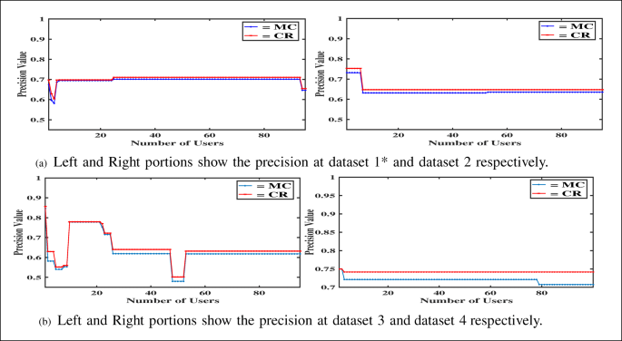
The graph shows the comparison between MC and CR at 15% sparsity. In most of the observations, the precision value of MC and CR is not overlapped and the precision value of CR is greater than the precision value of MC. It implies that CR is a more favorable approach than MC
The analysis of the precision values at different levels of sparsity also depicts nearly the same scenario as the previous analysis put forward. It becomes clear that the precision of CR gets better than MC and gradually surpasses it. Recall also varies on a scale of 0 to 1. Comparison of recall values at different level of sparsity are illustrated in Figs. 16, 17 and 18.
Fig. 16 
The graph represents the comparison between MC and CR based on recall value at 5% sparsity. Most of the users have higher recall value of CR than MC. This condition is sufficient to support that CR is more accurate in this sparse dataset
Fig. 17 
The graph shows the comparison between MC and CR on the basis of recall value at 10% sparsity. The recall value of CR is greater than MC in all the observations. Hence, CR is more accurate at 10% sparsity also
Fig. 18 
The graph portrays the comparison between MC and CR on the basis of recall value at 15% sparsity. It can be clearly observed that the recall value of CR is higher than MC. Thus, the CR approach is more favorable for rating prediction
Throughout the above Figs. 16 to 18, the proposed approach proves to be more effective in rating prediction than the Mean Centering approach.
-
Comparison of MC and CR using Standard Error (SE) and p-value In addition, to the above accuracy measures, we have also considered SE and p-value. SE of an estimator is nothing but the estimated standard deviation of the mean of the sample. Suppose we draw the N number of repeated samples, then it is expected that the SD of those sample means should be closer to the SE of the same. We can estimate the SE of the sample mean distribution as the sample SD divided by the square root of the size of the sample, which can be written as follows [59,60,61]:
$$ SE = \frac{SD}{\sqrt[2]{N}} $$(10)Probability of (|T| > |t|) is the computed p-value using the t distribution under two-tailed test [59,60,61]. It is nothing but the observing probability of a greater absolute value of t under the null hypothesis. If the computed p-value is lesser than the value of tabulated alpha level (normally 0.01 or 0.05 etc.) then we can conclude that the mean difference is statistically significant. However, Probability of (T < t) and Probability of (T > t) are p-values to evaluate the alternatives of (mean < H0) and (mean > H0) respectively under one-tailed test. In Table 11, the SE and p-value of CR is less than that of MC. Thus, we can conclude that CR is less prone to be erroneous.
Table 11 Results of the estimations of missing values The aforementioned graphical plots (from Figs. 10 to 18) and Table 11 are illustrating that the predictions of rating performed using Congenrous Rating approach provides better accuracy than those predictions performed using Mean Centering approach.
-
-
2.
Comparison of MC and CR based on their running complexity CR becomes more preferable approach since CR takes \(\mathcal {O}(n(n + m))\) whereas, MC utilizes \(\mathcal {O}(n(n + mlogn))\) time in best case.
-
Comparison of MC and CR based on the average standard deviation of items
The comparison of MC and the proposed prediction approach (CR) based on the average standard deviation of items’ rating are shown in Figs. 19 to 22. The above graphs examine the affinity of predicted value towards the mean rating of the target item for both MC and CR. Now, the increase in sparsity from 10% to 70% reveals a stronger bias of MC towards mean of the target item in comparison with CR.
-


The graph portrays the comparison of MC and CR at different levels of sparsity on dataset 1*

The graph portrays the comparison of MC and CR at different levels of sparsity on dataset 2

The graph portrays the comparison of MC and CR at different levels of sparsity on dataset 3

The graph portrays the comparison of MC and CR at different levels of sparsity on dataset 4
As we discussed earlier, MC outperforms the other traditional prediction approaches on the basis of accuracy in rating prediction. For rating prediction, the equation of MC in item-based CF can be divided into two parts with sum operation: (i) the mean rating of the target item, and (ii) dividing the weighted sum of ratings of the k most similar items by the sum of all the similarity values of the k most similar items. For moderately sparse dataset 1* from Fig. 19, we can notice that the average standard deviation of all items after the predicted rating using MC is far away from zero. This nature of predicted rating can be due to the existing similarity value between items that provides a nonzero value of the second part in MC approach. In this scenario, the predicted rating of target item gets some difference from its mean rating. But, with the increasing sparsity, the similarity measure faces difficulty in finding of similarity value between items. Therefore, Patra et al. have proposed a new similarity measure (BC) that mitigates the limitation of existing similarity measures by providing the similarity value between items in a sparse scenario. But, for a large number of similar items, the sum of the similarity values of k most similar items, used in the second part of the MC approach becomes very large. Hence, the second part of the MC approach will highly tend toward the zero value. In such scenario, the predicted rating of the target item will be equal to the mean rating of the target item in the MC approach and the average standard deviation of an item will incline towards zero.
To mitigate the above limitation, the proposed prediction approach uses only the similarity value of the ‘most’ similar item and the rating of the ‘most’ similar item. The rationale behind considering the ‘most’ similar item in the proposed work is summarized as: (i) Item-item correlation matrix generated using correlation measure such as Pearson correlation or its variants may be positive or positive semi definite matrix for which all Eigenvalues are positive or non-negative. Therefore, the determinant of the correlation matrix always lies between 0 and 1 and inclusive. (ii) If the value of the determinant is below certain threshold value, then the matrix will be collinear. However, sparsity in the large dataset causes most of the item-item correlation matrix non-collinear. In such scenario, Principle Component Analysis (PCA) and Orthogonal transformation can be used to find the optimal value k nearest neighbor for different target item which is computationally expensive.
From Section 5.1.1, it is observed that for all the considered datasets, the proposed CR outperforms MC. Hence, the similarity measure using the Bhattacharyya co-efficient, and the proposed prediction approach enhance the accuracy of existing item-based CF.
6 Conclusion and future work
The efficiency of business analytics is much dependent on the success of RS. The impact of RS in CF technique is influenced more by the prediction accuracy rather than the similarity in the sparse dataset. The accuracy of the existing prediction approaches used in item-based collaborative filtering is not impressive for a large value of k in most similar items, since the predicted rating of the target item may tend to mean or zero leading to lesser accuracy in the result. In such a scenario, if the prediction is done using the ‘most’ similar item, the accuracy improves significantly as the predicted rating shifts from the mean rating of the target item. The proposed approach provides a two-fold advantage, viz. providing better accuracy than the best of the prominent prediction approaches and secondly, a more personalized recommendation as average similar item ratings are no more taken into consideration.
Several experiments were conducted on three popularly used data sets to demonstrate the effectiveness of the proposed approach. From the experimental results, we observed that the proposed prediction approach can perform better than the existing methods. These results demonstrate the effectiveness of the proposed method and it successfully overcame the drawbacks of the existing prediction approaches. According to the experimental results, the proposed prediction approach significantly outperformed the traditionally best prediction approach in terms of precision, recall, F1, MAE, RMSE, SE, and p-value etc. even when the similarity is calculated using the Bhattacharrya coefficient. Hence, we conclude that the idea of selecting most similar item of a target item contributes more to the prediction of accurate and personalized items which target users may prefer.
Mere accuracy in the statistical analysis will not always lead to an efficient recommendation as it may not reflect the personal taste of the user. Therefore, the future scope of the work will be to extract the intensity of users’ choice depending on the features of the item for a fully matured and accurate recommendation. The recommendation list may contain diversified items as proposed by Jain et al. In this direction, diversity and accuracy of recommendation will be more enhanced using the combination of the multi-objective similarity model by Jain et al., and our modified prediction approach (i.e. ‘most’ similar neighbor).
References
Recommender systems. http://www.cs.carleton.edu/cs_comps/0607/recommend/recommender/modelbased.htmlhttp://www.cs.carleton.edu/cs_comps/0607/recommend/recommender/modelbased.html, [Online; accessed 17-August-2019]
Choi K, Suh Y (2013) A new similarity function for selecting neighbors for each target item in collaborative filtering. Knowl-Based Syst 37:146–153
Karypis G (2001) Evaluation of item-based top-n recommendation algorithms. In: Proceedings of the Tenth international conference on information and knowledge management, CIKM ’01, pp 247–254
Liu H, Hu Z, Mian AU, Tian H, Zhu X (2014) A new user similarity model to improve the accuracy of collaborative filtering. Knowl-Based Syst 56:156–166
Collaborative filtering. https://en.wikipedia.org/wiki/Collaborative_filteringhttps://en.wikipedia.org/wiki/Collaborative_filtering, [Online; accessed 12-November-2017]
Comparison of user-based and item-based collaborative filtering. [Online; accessed 17-August-2019]. https://medium.com/@wwwbbb8510/comparison-of-user-based-and-item-based/-collaborative-filtering-f58a1c8a3f1dhttps://medium.com/@wwwbbb8510/comparison-of-user-based-and-item-based/-collaborative-filtering-f58a1c8a3f1dhttps://medium.com/@wwwbbb8510/comparison-of-user-based-and-item-based/-collaborative-filtering-f58a1c8a3f1d
Sarwar B, Karypis G, Konstan J, Riedl J (2001) Item-based collaborative filtering recommendation algorithms. In: Proceedings of the 10th international conference on World Wide Web, ACM, pp 285–295
Yang Z, Wu B, Zheng K, Wang X, Lei L (2016) A survey of collaborative filtering-based recommender systems for mobile internet applications. IEEE Access 4:3273–3287
Linden G, Jacobi J, Benson E (2001) Collaborative recommendations using item-to-item similarity mappings. [Google Patents]
Deshpande M, Karypis G (2004) Item-based top-n recommendation algorithms. ACM Trans Inf Syst 22(1):143–177
Patra BK, Launonen R, Ollikainen V, Nandi S (2015) A new similarity measure using bhattacharyya coefficient for collaborative filtering in sparse data. Knowl-Based Syst 82:163–177
Li D, Miao C, Chu S, Mallen J, Yoshioka T, Srivastava P (2018) Stable Matrix Approximation for Top-N Recommendation on Implicit Feedback Data
Xu J, Man H (2011) Dictionary learning based on laplacian score in sparse coding. In: Machine learning and data mining in pattern recognition - 7th international conference, pp 253–264
Bobadilla J, Hernando A, Ortega F, Gutiérrez A (2012) Collaborative filtering based on significances. Inf Sci 185(1):1–17
Ricci F, Rokach L, Shapira B, Kantor PB (2010) Recommender systems handbook, 1st edn. Springer, New York
Lu J, Yue J, Zhu L, Li G (2019) Variational mode decomposition denoising combined with improved bhattacharyya distance. Measurement 151:107283
Wu J, Chen L, Feng Y, Zheng Z, Zhou M, Wu Z (2013) Predicting quality of service for selection by neighborhood-based collaborative filtering. IEEE Trans Systems, Man, and Cybernetics: Systems 43 (2):428–439
Herlocker J, Konstan JA, Riedl J (2002) An empirical analysis of design choices in neighborhood-based collaborative filtering algorithms. Inf Retr 5:287–310
Herlocker JL, Konstan JA, Borchers A, Riedl J (1999) An algorithmic framework for performing collaborative filtering. In: Proceedings of the 22nd annual international ACM SIGIR conference on research and development in information retrieval, pp 230–237
Kim H-N, Ji A-T., Kim H-J, Jo G-S (2007) Error-Based collaborative filtering algorithm for Top-N recommendation
Ahn HJ (2008) A new similarity measure for collaborative filtering to alleviate the new user cold-starting problem. Inf Sci 178(1):37–51
i Mansilla AT, de la Rosa i Esteva JL (2012) Asknext: an agent protocol for social search. Inf Sci 190:144–161
Shen K, Liu Y, Zhang Z, Lu W (2017) Modified similarity algorithm for collaborative filtering. In: Uden L, Ting I-H (eds) Knowledge management in organizations. Springer International Publishing, pp 378–385
Palak R, Nguyen NT (2017) An effective collaborative filtering based method for movie recommendation, pp 149–159
Boratto L, Carta S, Fenu G (2017) Investigating the role of the rating prediction task in granularity-based group recommender systems and big data scenarios. Inf Sci 378:424–443
Koohi H, Kiani K (2017) A new method to find neighbor users that improves the performance of collaborative filtering. Expert Syst Appl 83:30–39
Stephen SC, Xie H, Rai S (2017) Measures of similarity in memory-based collaborative filtering recommender system: A comparison. In: Proceedings of the 4th Multidisciplinary International Social Networks Conference, ACM, pp 32:1–32:8
Liu Y, Feng J, Lu J (2017) Collaborative filtering algorithm based on rating distance. In: Proceedings of the 11th International Conference on Ubiquitous Information Management and Communication, ACM, pp 66:1–66:7
Ai J, Li L, Su Z, Wu C (2017) Online-rating prediction based on an improved opinion spreading approach. In: 29Th chinese control and decision conference
Birtolo C, Ronca D (2013) Advances in clustering collaborative filtering by means of fuzzy c-means and trust. Expert Syst Appl 40(17):6997–7009
Ghazarian S, Nematbakhsh MA (2015) Enhancing memory-based collaborative filtering for group recommender systems. Expert Syst Appl 42(7):3801–3812
Guo G (2013) Integrating trust and similarity to ameliorate the data sparsity and cold start for recommender systems. In: Seventh ACM conference on recommender systems, RecSys ’13, pp 451–454
Guo G, Zhang J, Thalmann D (2014) Merging trust in collaborative filtering to alleviate data sparsity and cold start. Knowl-Based Syst 57:57–68
Sun D, Luo Z, Zhang F (2011) A novel approach for collaborative filtering to alleviate the new item cold-start problem. In: 11th International Symposium on Communications and Information Technologies, ISCIT, pp 402–406
Jorge AM, Vinagre J, Domingues M, Gama J, Soares C, Matuszyk P, Spiliopoulou M (2017) Scalable online Top-N recommender systems. Springer International Publishing
Geuens S, Coussement K, De Bock KW (2018) A framework for configuring collaborative filtering-based recommendations derived from purchase data. Eur J Oper Res 265(1):208–218
Adamopoulos P (2013) Notes on recommender systesm: a survey of state-of-the-art algorithms, beyond rating prediction accuracy approaches and business value perspectives
Lohr SL (2009) Sampling: Design and Analysis. 2nd Edn, Cengage Learning
Bobadilla J, Ortega F, Hernando A (2012) A collaborative filtering similarity measure based on singularities. Inform Process Manage 48(2):204–217
Liu Y, Feng J, Lu J (2017) Collaborative filtering algorithm based on rating distance. In: Proceedings of the 11th International Conference on Ubiquitous Information Management and Communication, pp 1–7
Cacheda F, Carneiro V, Fernández D, Formoso V (2011) Comparison of collaborative filtering algorithms: Limitations of current techniques and proposals for scalable, high-performance recommender systems. ACM Trans Web 5(1):2:1–2:33
Bilge A, Kaleli C (2014) A multi-criteria item-based collaborative filtering framework. In: 11th international joint conference on computer science and software engineering (JCSSE), pp 18– 22
Hui S, Pengyu L, Kai Z (2011) Improving item-based collaborative filtering recommendation system with tag. In: 2nd International Conference on Artificial Intelligence, Management Science and Electronic Commerce (AIMSEC), pp 2142–2145
Wen J, Zhou W (2012) An improved item-based collaborative filtering algorithm based on clustering method. J Compute Inform Syst, pp 571–578
Koohi H, Kiani K, new method to find neighbor users A (2017) That improves the performance of collaborative filtering. Expert Syst Appl 83:30–39
Ye F, Zhang H (2016) A collaborative filtering recommendation based on users’ interest and correlation of items. In: International conference on audio, language and image processing (ICALIP), pp 515–520
Suryakant T, Mahara A (2016) New similarity measure based on mean measure of divergence for collaborative filtering in sparse environment. Procedia Computer Science 89:450–456
Ayub M, Ghazanfar MA, Maqsood M, Saleem A (2018) A jaccard base similarity measure to improve performance of cf based recommender systems. In: International conference on information networking (ICOIN), IEEE, pp 1–6
Al-Bashiri H, Abdulgabber MA, Romli A, Kahtan H An improved memory-based collaborative filtering method based on the topsis technique, PloS One 13 (10)
Ding Y, Li X (2005) Time weight collaborative filtering. In: Proceedings of the 14th ACM international conference on Information and knowledge management, ACM, pp 485–49
Zhang Z-P, Kudo Y, Murai T, Ren Y-G (2019) Enhancing recommendation accuracy of item-based collaborative filtering via item-variance weighting. Appl Sci 9(9):1928
Gao M, Wu Z, Jiang F (2011) Userrank for item-based collaborative filtering recommendation. Inf Process Lett 111(9):440– 446
Jain A, Singh P, Dhar J (2019) Multi-objective item evaluation for diverse as well as novel item recommendations. Expert Systems with Applications 139:112857
Linden G, Smith B, York J (2003) Amazon.com recommendations: Item-to-item collaborative filtering. IEEE Internet Computing 7(1):76–80
Paterek A (2007) Improving regularized singular value decomposition for collaborative filtering. In: Proceedings of KDD cup and workshop, vol 2007, pp 5–8
Lin D (1998) An information-theoretic definition of similarity. In: Proceedings of the Fifteenth international conference on machine learning, pp 296–304
Alqadah F, Reddy CK, Hu J, Alqadah HF (2015) Biclustering neighborhood-based collaborative filtering method for top-n recommender systems. Knowl Inf Syst 44(2):475–491
Gunawardana A, Shani G (2009) A survey of accuracy evaluation metrics of recommendation tasks. J Mach Learn Res 10:2935–2962
Venables WN, Ripley BD (2002) Modern applied statistics with S, 4th edn. Springer, New York
Givens GH, Hoeting JA (2005) Computational Statistics. 2nd Edn, Wiley
Martinez WL, Martinez AR (2007) Computational statistics handbook with MATLAB. 2nd Edn, Chapman and Hall/CRC
Author information
Authors and Affiliations
Corresponding author
Additional information
Publisher’s note
Springer Nature remains neutral with regard to jurisdictional claims in published maps and institutional affiliations.
Rights and permissions
About this article

Cite this article
Singh, P.K., Sinha, M., Das, S. et al. Enhancing recommendation accuracy of item-based collaborative filtering using Bhattacharyya coefficient and most similar item. Appl Intell 50, 4708–4731 (2020). https://doi.org/10.1007/s10489-020-01775-4
Published:
Issue Date:
DOI: https://doi.org/10.1007/s10489-020-01775-4