
Abstract
An interval type-2 fuzzy weighted support vector machine (IT2FW-SVM) is proposed to address the problem of high energy consumption for biped walking robots. Different from the traditional machine learning method of ‘copy learning’, the proposed IT2FW-SVM obtains lower energy cost and larger zero moment point (ZMP) stability margin using a novel strategy of ‘selective learning’, which is similar to human selections based on experience. To handle the uncertainty of the experience, the learning weights in the IT2FW-SVM are deduced using an interval type-2 fuzzy logic system (IT2FLS), which is an extension of the previous weighted SVM. Simulation studies show that the existing biped walking which generates the original walking samples is improved remarkably in terms of both energy efficiency and biped dynamic balance using the proposed IT2FW-SVM.
1 Introduction
Energy efficiency is a fatal problem for the practical application of biped robots. Control methods based on the ZMP theory are already comparatively mature, while actuated bipods such as ASIMO [1] of Honda, needs tens of times as much energy as humans need. Passive dynamic walking (PDW) provided clues to solve the problem of generating a natural and energy efficient gait [2]. However, it is difficult to achieve complex dynamics, and a very small disturbance may lead to failure. Semi-passive walkers [3, 4] maintain walking with a minimum amount of joint control. They introduce some robustness and they can walk without a slope. However, the semi-passive walkers are less capable and less robust relative to fully actuated walkers.
Recently, from the point of machine learning, several approaches have been proposed to generate biped gaits that ensure maximum dynamic balance margin and minimum power consumption. In the literatures [5–7], the GA (genetic algorithm), the PSO (particle swarm optimization) algorithm, an approach of GA-FL (genetic-algorithm-trained fuzzy logic) and an approach of GA-NN (genetic-algorithm-trained neural network) are applied to optimize the energy cost and the ZMP stability of a biped robot. These studies provided promising results for energy efficient biped walking on rough terrain.
On the other hand, some researchers have proposed significant solutions for biped dynamic balance using the support vector machine (SVM), which has been proved to possess remarkable characteristics of good generalization performance, the absence of local minima, and sparse representation of solution [8–16]. Instead of the standard SVMs, we find interesting clues to learn biped walking locomotion with both low energy consumptions and dynamic balance using weighted SVMs. Weighted SVMs increase the importance of certain training points by assigning bigger learning weights to the concerned samples [17–21], it is a typical way to realize the ‘selective learning’. There is no formulaic way of designing the learning weights of samples. Different criteria such as ‘error variables’ [17], ‘number of examples’ [18], ‘approximate entropy’ [19], ‘posterior probability’ [20] and ‘distance’ [21] are proposed to design weights of the weighted SVM. As we can see, designing the weights is a key issue in weighted SVMs, and appropriate methods must be proposed to solve various problems.
To address the problem of weight-designing for energy efficient biped walking, fuzzy logic systems (FLSs) are considered because there exist complex uncertainties in the evaluation criteria for the biped walking samples and the biped walking samples themselves, and FLSs are powerful tools for handling uncertainties. Some studies on fuzzy weighted SVM have previously been presented [22–26]. However, most of previous researches have focused on type-1 FLSs, although type-2 FLSs [27–32] appears to be a more promising method than their type-1 [33–35] counterparts for handling uncertainties in rule-based systems.
In this work, an IT2FW-SVM is proposed to cope with the fatal problem of high energy consumption for biped walking robots. The training samples are evaluated by two important indexes (the energy cost and the ZMP stability margin of biped walking robots). The principle of designing the learning weights is that samples with better performances are treated as more important ones in the training. Considering the numerical and linguistic uncertainty from original data and the evaluation mechanism, the learning weights are deduced using an IT2FLS. As a result, walking samples with lower energy cost and larger ZMP stability margin contribute more to the learning of the energy efficiency biped walking. Using the proposed IT2FW-SVM, the existing biped walking which generates the original walking samples is improved remarkably in terms of both energy efficiency and biped dynamic balance.
Main contributions of this work could be summarized as follows:
-
High energy consumption is a fatal problem for the practical application of biped robots. The proposed approach provides a novel clue to address this problem.
-
The weights in the IT2FW-SVM are determined by two important indexes of biped walking (the energy cost and the ZMP stability margin). This strategy has not been reported before.
-
To handle the complex uncertainties of biped systems, the learning weights in the IT2FW-SVM are deduced using an IT2FLS, which is an extension of the previous weighted SVM.
The organization of this paper is as follows. In Sect. 2, the background about the energy cost and the dynamic balance of biped robots are represented. An IT2FW-SVM learning system for biped robots is designed in Sect. 3. Simulation results are provided in Sect. 4, followed by the conclusions in Sect. 5.
2 Primary features of biped walking
2.1 Energy cost of the joints
Energy efficiency is an important problem which has been recognized as one of the central problems for biped walkers today. In order to achieve energy efficient biped walking, performance indexes of energy consumption for biped walking robots are defined here first. There are two common indexes for energy consumption of biped robots [36], which can be calculated as follows:
where S is the mechanical energy cost of biped robots, E is the torque cost of the biped joints. \(\dot{\theta}\) is a joint velocity, and τ is a control torque of biped joints. t start and t end are the beginning and the ending time for the energy cost of biped robots. The energy consumption index shown in Eq. (1) characterizes the variation of the mechanical energy of the system. It is less dependent on the driving actuator. No brake is used, so the negative work must be produced by the actuators. Therefore the absolute value of the work is considered. The index shown in Eq. (2) characterizes the energy that must be produced by the battery to allow the biped motion. In this work, the primary consideration is the energy cost shown in Eq. (2).
2.2 ZMP stability margin
Dynamic balance of legged systems is analyzed according to the concept of ZMP introduced by Vukobratovic et al. in 1990. ZMP is defined as that point on the ground at which the net moment of the inertial forces and the gravity forces has no component along the horizontal axes. At a given time instant, the ZMP position is influenced by all the forces acting on the system. The dynamic balance of the system is ensured if the ZMP is inside the support area [37].
To avoid having only one edge of the foot sole contacting the ground, there should be some distance between the actual ZMP and the boundary of the support area. In the following, the minimum distance between the ZMP and the boundary of the support area is called the ZMP stability margin.
The ZMP can be computed using the following equations:
where (x zmp ,y zmp ,0) is the coordinate of the ZMP, and (x i ,y i ,z i ) is the coordinate of the mass center of link i on an absolute Cartesian coordinate system. m i is the mass of link i, I ix and I iy are the inertial components, Ω ix and Ω iy are the absolute angular accelerations components around x axis and y axis at the center of gravity of link i, g is the gravitational acceleration.
3 Learning energy efficient biped walking using the IT2FW-SVM
Using the proposed IT2FW-SVM, we try to improve the existing biped walking which generates the original walking samples. The original walking samples are generated by a proportion-integration-differentiation (PID) [38] controller according to the planned gait, and the IT2FW-SVM is trained offline. Using the energy cost and the ZMP stability margin as inputs, and the learning weights as outputs, an IT2FLS provides a comprehensive criterion to the IT2FW-SVM for ‘selective learning’. By learning the weighted walking samples evaluated by the IT2FLS, the IT2FW-SVM obtains regression equations for energy efficient control torque of the key joints (the supporting hip and the supporting ankle), which are used to realize the energy efficient biped walking.
3.1 Biped dynamic to be built using the IT2FW-SVM
In the single support phase (SSP), the effective control of the supporting ankle and the supporting hip plays a key role in ensuring the dynamic biped balance. When the ZMP criterion is satisfied, the dynamic between the driving torque and the joint angles can be written as [39]:
where U EE (⋅) and V EE (⋅) are the energy efficient nonlinear dynamic that the IT2FW-SVM tries to build. τ sup_hip and τ sup_ankle are driving torques, θ sup_hip and θ sup_ankle are joint angles.
3.2 Objective functions of the IT2FW-SVM
In the objective functions of the IT2FW-SVM, the most important thing is that an IT2FLS [40] is used to design learning weights for each sample. Taking the learning of driving torque of the supporting hip as an example, designing a learning weight d l for each of the training samples, and the training sample set can be denoted as \(\{ \theta_{\sup \_hip}^{(l)},\theta_{\sup \_ankle}^{(l)}, \tau_{\sup \_hip}^{(l)},d_{l}\}\), 0≤d l ≤1, l=1,2,…,N. Then the IT2FW-SVM objective function for regressing the driving torque of the supporting hip is
where ω is a weight vector. ϕ(⋅) is a nonlinear mapping function for mapping the input space into a higher dimension feature space. C is a penalty coefficient, ξ l and \(\xi_{l}^{*}\) are positive slack variables enabling the objective functions to deal with permitted errors, N is the number of the samples. (\(\theta_{\sup \_hip}^{(l)},\theta_{\sup \_ankle}^{(l)}\)) are the input vectors and \(\tau_{\sup \_hip}^{(l)}\) is the output of the lth sample. b sup_hip is the corresponding bias. d l is the learning weight to be designed in the next section.
3.3 Designing the learning weights using an IT2FLS
This section designs the learning weights of the IT2FW-SVM using an IT2FLS. The antecedent part of the IT2FLS uses interval type-2 fuzzy sets, and the consequent part is of the Mamdani-type. The ith rule in the system has the following form:
where e and z are the energy cost and the ZMP stability margin respectively, d is the learning weights of the IT2FW-SVM. \(\tilde{A}_{i,j}\), j=1,…,n is an interval type-2 fuzzy set, \(\tilde{G}_{i}\) is the output interval type-2 fuzzy set of the ith rule, and M is the number of rules. Based on the rule base in (8), the computation of the IT2FLS involves the fuzzifier, inference engine, type reducer, and defuzzifier, which will be described in detail next.
3.3.1 Fuzzification
The fuzzifier maps crisp input values to fuzzy sets. For the ith fuzzy set \(\tilde{A}_{i,j}\) in the input variables, a Gaussian primary membership function is used, which has a fixed standard deviation σ and an uncertain mean that takes on values in [\(\underline{m},\bar{m}\)].
For example, the membership degree of the energy cost is
Here, the membership degree \(\mu_{\tilde{A}_{i,j}}(e_{j})\) is an interval set and is denoted by \(\mu_{\tilde{A}_{i,j}}(e_{j}) = [\underline{\mu}_{\tilde{A}_{i,j}}(e_{j}),\bar{\mu}_{\tilde{A}_{i,j}}(e_{j})]\). The mathematical functions of the lower and upper MFs, \(\underline{\mu}_{\tilde{A}_{i,j}}(e_{j})\) and \(\bar{\mu}_{\tilde{A}_{i,j}}(e_{j})\), are described as follows:
Similarly, the membership degree of the ZMP stability margin can be expressed as
And the membership degree of the learning weights can be expressed as
3.3.2 Inference
The inference engine operation performs the fuzzy meet operation by using an algebraic product operation. The result of the input and antecedent operations F i is an interval type-1 set, \(\mathrm{i}.\mathrm{e}.,F_{i} = [\underline{f}_{i},\bar{f}_{i}]\), where
The ith rule fired output consequent set
where \(\bar{\mu}_{\tilde{G}_{i}}(d)\) and \(\underline{\mu}_{\tilde{G}_{i}}(d)\) are the lower and upper membership grades of \(\mu_{\tilde{G}_{i}}(d)\). The output fuzzy set \(\mu_{\tilde{B}}(d)\) is
where ‘∨’ operation is the maximum operation.
3.3.3 Type reduction
For IT2FLSs, the final crisp output is the center of the type-reduced set. There exist many kinds of type-reduction, such as centroid, center-of-sets, height, and modified height [40]. In this paper, center-of-sets type-reduction is used as follows:
where low and high represent the left and right limits, respectively. d i is the centroid of the type-2 interval consequent set \(\tilde{G}_{i}\).
There is no direct theoretical solution for Eq. (17). The computation of the reduced set requires an iterative procedure. This paper computes Eq. (17) using the Karnik-Mendel iterative procedure, which consists of an initialization step followed by four iterative steps [41]. In this procedure, the rule’s consequent parts should first be arranged in ascending order. Let d=(d 1,…,d M ) denote the original rule-ordered consequent values and let \(\tilde{d} = (\tilde{d}_{1}, \ldots,\tilde{d}_{M})\) denote the reordered sequence, where \(\tilde{d}_{1} \le \tilde{d}_{2} \le \cdots \le \tilde{d}_{M}\). The relationship between d and \(\tilde{d}\) can be represented as \(\tilde{d} = Qd\), where Q is an M×M permutation matrix. This permutation matrix uses elementary vectors as columns, and these vectors are arranged to move elements in d to new locations in ascending order in the transformed vector \(\tilde{d}\). Reorder the original rule firing strength orders \(\underline{f} = (\underline{f}_{1},\underline{f}_{2}, \ldots,\underline{f}_{M})^{T}\) and \(\bar{f} = (\bar{f}_{1},\bar{f}_{2}, \ldots,\bar{f}_{M})^{T}\) accordingly, and the new orders become \(Q\underline{f}\) and \(Q\bar{f}\), respectively. The outputs d low and d high can be computed as follows:
where L and R denote the left and right crossover points, respectively. These two points vary with different inputs. Karnik-Mendel iterative procedure can be used here to find these two points.
3.3.4 Defuzzification
The defuzzifier computes the system output variable d by performing the defuzzification operation on the interval set [d low ,d high ] from the type reduction. Based on the centroid defuzzification operation, the centroid of the interval set [d low ,d high ] is the average of d low and d high . Hence, the defuzzified output is
Up to now, with type-2 fuzzy inputs of the energy cost and the ZMP stability margin for biped robots, the corresponding learning weight of the biped walking sample is deduced using an IT2FLS. The deduced learning weights are then used in the learning process of the IT2FW-SVM as shown in the next section.
3.4 Learning algorithms of the IT2FW-SVM
To solve the proposed optimization problem in Eq. (7), we construct the Lagrangian
and find the saddle point of L(ω,b,ξ,α). The parameters must satisfy the following conditions:
eliminating ω and ξ using Eq. (22), the problem Eq. (7) can be transformed into
where \(\tau_{\sup \_hip} = [\tau_{\sup \_hip}^{(1)},\tau_{\sup \_hip}^{(2)}, \ldots,\tau_{\sup \_hip}^{(N)}]^{T}\), A=[1,1,…,1]T, α=[α 1,α 2,…,α N ]T, Ω is a square matrix, which has elements of
Submitting the optimal α and b sup_hip , the regression function of the IT2FW-SVM for learning the driving torque of the supporting hip is
where τ sup_hip is the energy efficient driving torque of the supporting hip. b sup_hip is the corresponding bias. α l ≥0, l=1,…,N are Lagrangian multipliers, N is the number of the samples. K(⋅) is a kernel function. Here, the Gaussian kernel
is used, where σ is the width of the Gaussian kernel. Using the same algorithm presented in this section, IT2FW-SVM learning results for the energy efficient driving torque of the supporting ankle can be obtained as follows:
4 Simulation research
In this section, we test our proposed IT2FW-SVM system on the learning of a seven-link biped walking in the sagittal plane by simulation experiments. Data of the implemented biped robot are given from the GDUT-I biped robot, which is designed and built at the Faculty of Automation, Guangdong University of Technology, Guangzhou, Guangdong, China. Details about GDUT-I biped robot can be found in the literature [42].
4.1 Generating sample sets
There are 160 groups of walking samples in the simulations. The first 120 groups are chosen for training and the last 40 groups are chosen for test. Sample sets for the IT2FW-SVM include three parts: the joint angles, the driving torques and the learning weights. The way we get all the three parts of the training data is described in detail next.
4.1.1 Joint angles
The joint angles come from reference trajectory planned offline.
The walking period of the biped robot is planned to be composed of a SSP and an instantaneous double support phase (DSP). The supporting foot remains in full contact with the ground during the SSP. The walk cycle is T c =1 s. Three different motions are considered: Motion1 has a step length of 0.16 m, motion2 has a step length of 0.18 m, and motion3 has a step length of 0.20 m. The three motions have the same step height of 0.02 m. The trajectories are represented as follows:
where x hip ,z hip represents the position of the hip and x ankle ,z ankle represents the position of the swinging ankle joint. s denotes the walking step length, and q denotes the height of swinging ankle. N denotes the total sampling number for a step, l denotes the sampling index, and l thigh ,l shank represent the length of lower limbs.
4.1.2 Driving torques
The driving torques are obtained using a PID controller.
In this work, the initial driving torques of all the joints are obtained using a PID controller. Then the key driving torques, including driving torques for the support hip and support ankle, are improved using the proposed IT2FW-SVM. The initial driving torques of all the joints are obtained using the following PID controller:
where τ j (j=1,…,n,n=7) is the torque of the joints. e j denotes the offset of the desired reference trajectories and the actual trajectories. The integral period is T=0.025 s. The proportional gains P j , integral gains I j and differential gains D j are slightly modified by the trial-error method. The parameters are shown in Table 1.
4.1.3 Learning weights
The learning weights are obtained using an IT2FLS, which has the energy cost and the ZMP stability margin as inputs, and the learning weights as outputs. The ith rule in the system has the following form:
where e and z are the energy cost and the ZMP stability margin, respectively. d is the learning weights of the IT2FW-SVM. \(\tilde{A}_{i,j}\), j=1,…,5 is an interval type-2 fuzzy set, \(\tilde{G}_{i}\) is the output interval type-2 fuzzy set of the ith rule, and the number of rules is 25.
Here, two steps are involved in the derivation procedures of the fuzzy rules. Firstly, primary fuzzy rules are initialized by expert experience. Secondly, the final fuzzy membership functions are obtained through fine adjustments according to the experimental data. The principle of designing the learning weights is that samples with better features are treated as more important ones in the training. So, larger learning weights are assigned to walking samples with less energy cost and larger ZMP stability margin. The rule base for the weights designing is shown in Table 2.
The details about Table 2 will be described next:
-
(1)
Energy cost of the biped joints can be calculated using Eq. (2). To express the linguistic and numerical uncertainty, interval type-2 fuzzy membership functions of the energy cost are designed as Fig. 1. Gaussian primary membership functions are used, which have a fixed standard deviation σ=50 and uncertain means that take on values in the following intervals:
$$\begin{aligned} & \bigl[\underline{m}_{i1}^{e}, \bar{m}_{i1}^{e} \bigr] = [0,10], \quad \bigl[ \underline{m}_{i2}^{e},\bar{m}_{i2}^{e} \bigr] = [100.63,110.63] \\ & \bigl[ \underline{m}_{i3}^{e},\bar{m}_{i3}^{e} \bigr] = [206.25,216.25] \\ & \bigl[\underline{m}_{i4}^{e},\bar{m}_{i4}^{e} \bigr] = [311.88,321.88] \\ & \bigl[\underline{m}_{i5}^{e}, \bar{m}_{i5}^{e} \bigr] = [417.5,427.5] \end{aligned} $$The domain of the energy cost is
$$ [e_{\min},e_{\max} ] = \bigl[0,422.5~\mbox{N}^{2}\,\mbox{m}^{2} \bigr] $$(30)Here, each servomotor in the implemented biped joint has a maximum torque of 130 N m, so the corresponding maximum energy cost is
$$ e_{\max} = \int_{t}^{t + 0.025} ( 130~\mbox{N}\,\mbox{m})^{2} dt = 422.5\ \bigl(\mbox{N}^{2}\,\mbox{m}^{2} \bigr) $$(31)Fig. 1 
Interval type-2 fuzzy membership function of the energy cost
-
(2)
The ZMP stability margin can be deduced using the ZMP position calculated by Eq. (3). Considering the linguistic and numerical uncertainty of the system, interval type-2 fuzzy membership functions of the ZMP stability margin are designed as Fig. 2. In the SSP, the maximum ZMP stability margin is half of the foot-length in the sagittal plane, which is 0.04 m for the implemented biped robot. So the domain of the ZMP stability margin is
$$ [z_{\min},z_{\max} ] = [0,0.04~\mbox{m}] $$(32)Also, Gaussian primary membership functions are used here, which have a fixed standard deviation σ=0.005 and uncertain means that take on values in the following intervals:
$$\begin{aligned} & \bigl[\underline{m}_{i1}^{z}, \bar{m}_{i1}^{z} \bigr] = [0,0.001] \\ & \bigl[\underline{m}_{i2}^{z}, \bar{m}_{i2}^{z} \bigr] = [0.0095,0.0105] \\ & \bigl[\underline{m}_{i3}^{z},\bar{m}_{i3}^{z} \bigr] = [0.0195,0.0205] \\ & \bigl[\underline{m}_{i4}^{z},\bar{m}_{i4}^{z} \bigr] = [0.0295,0.0305] \\ & \bigl[\underline{m}_{i5}^{z}, \bar{m}_{i5}^{z} \bigr] = [0.0395,0.0405] \end{aligned} $$Fig. 2 
Interval type-2 fuzzy membership function of the ZMP stability margin
-
(3)
The learning weight. The domain of the learning weight is specified as
$$ [d_{\min},d_{\max} ] = [0,1] $$(33)Interval type-2 fuzzy membership functions of the learning weights are designed as Fig. 3. Still, Gaussian primary membership functions are used, which have a fixed standard deviation σ=0.1 and uncertain means that take on values in the following intervals:
$$\begin{aligned} & \bigl[\underline{m}_{i1}^{d}, \bar{m}_{i1}^{d} \bigr] = [0,0.028], \quad \bigl[ \underline{m}_{i2}^{d}, \bar{m}_{i2}^{d} \bigr] = [0.156,0.184] \\ & \bigl[\underline{m}_{i3}^{d},\bar{m}_{i3}^{d} \bigr] = [0.316,0.344] \\ & \bigl[\underline{m}_{i4}^{d},\bar{m}_{i4}^{d} \bigr] = [0.486,0.514] \\ & \bigl[\underline{m}_{i5}^{d}, \bar{m}_{i5}^{d} \bigr] = [0.656,0.684] \\ & \bigl[\underline{m}_{i6}^{d},\bar{m}_{i6}^{d} \bigr] = [0.816,0.844], \quad \bigl[\underline{m}_{i7}^{d}, \bar{m}_{i7}^{d} \bigr] = [0.972,1] \end{aligned} $$Fig. 3 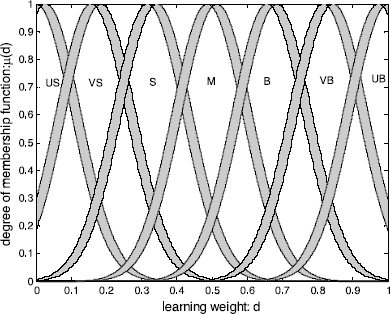
Interval type-2 fuzzy membership function of the learning weight


4.2 Hyper-parameters designing for the IT2FW-SVM
In general, the search algorithms used to obtain SVM hyper-parameters include grid search, local search and global optimization algorithms [43]. In this work, a 10-fold cross-validation strategy is applied to find the optimal hyper-parameters for the proposed IT2FW-SVM. The optimal hype-parameters of the IT2FW-SVM include a penalty factor C=1000, an insensitive loss parameter ε=0.001, the width of the Gaussian kernel σ=0.9.
Remark 1
Considering that all the search algorithms have the similar difficulty in the selection of the initial ranges for parameters, the literature [43] presents a novel study of the effect of including reductions in the range of SVM hyper-parameters, in order to reduce the SVM training time, but with the minimum possible impact in its performance. It will be interesting to improve the training time of support vector regression algorithms through novel hyper-parameters search space reductions in the future.
4.3 Performance analysis and comparisons
Two primary features of biped walking (described in the Sect. 2 of this paper, including the energy cost and the ZMP stability margin) are analyzed in this section.
4.3.1 Other methods to be compared with
Because we try to improve the existing biped walking using the proposed IT2FW-SVM, performance of the proposed method is first compared to the existing PID controller. Details of the PID controller can be found in Eq. (28).
Then, the IT2FW-SVM is compared to a standard SVM to show the effect of the ‘selective learning’ using learning weights. The standard SVM has an objective function expressed as:
where the symbols have the same definitions as those in Eq. (7).
On the other hand, to illustrate the necessity of adopting the IT2FLS in the proposed IT2FW-SVM, a type-1 fuzzy weighted SVM (T1FW-SVM) is presented for comparisons. The jth rule of the T1FW-SVM is expressed as follows:
where e and z are the energy cost and the ZMP stability margin respectively, d is the learning weights of the T1FW-SVM. A 1,j ,A 2,j ,and G j are type-1 fuzzy sets. Both the inputs and the outputs are fuzzified with Gaussian fuzzy membership functions, as shown in Fig. 4.

Type-1 fuzzy membership functions for the inputs and outputs. (a) Fuzzy membership functions for the inputs (the energy cost) with a fixed standard deviation σ=50 and fixed means of {m 1,m 2,m 3,m 4,m 5}={0.0,105.6,211.3,316.9,422.5}. (b) Fuzzy membership functions for the inputs (the ZMP stability margin) with a fixed standard deviation σ=0.005 and fixed means of {m 1,m 2,m 3,m 4,m 5}={0.00,0.01,0.02,0.03,0.04}. (c) Fuzzy membership functions for the outputs (learning weights) with a fixed standard deviation σ=0.1 and fixed means of {m 1,m 2,m 3,m 4,m 5,m 6,m 7}={0.00,0.17,0.33,0.50,0.67,0.83,1.00}
4.3.2 Analysis and comparisons of the energy cost
Energy cost of the supporting hip is considered as follows:
where \(\tau_{\sup \_hip}^{(l)}\) and \(E_{\sup \_hip}^{(l)}\) are energy cost and driving torque of the supporting hip on the lth sampling point in a walk cycle. t l−1 and t l are the beginning and ending time of the lth sampling interval, l=1,2,…,40. The whole energy-cost index expression is given as
Energy cost of the supporting ankle can be obtained in the same way.
Comparisons of the energy cost are shown in Table 3. The proposed IT2FW-SVM does the best when the energy cost performance index is analyzed, and simulation results show that all the gaits have a similar trend of increasing the energy cost as the step lengths increase. The energy cost performance of the standard SVM controller is very close to the PID controller, which is in line with the fact that the unweighted standard SVM is trained to mimic the PID one. On the other hand, by evaluating the energy cost of the samples and assign learning weights to the training samples accordingly, the T1FW-SVM controller reduces the energy cost to a certain degree. With further consideration, the proposed IT2FW-SVM translates the linguistic and numerical uncertainty from original data into fuzzy rules uncertainty, thus it enhances the energy efficiency of the biped robots remarkably, which demonstrates the effectiveness of the proposed IT2FW-SVM.
4.3.3 Analysis and comparisons of the dynamic biped balance
To analyze the performance index of the dynamic biped balance, mean of the ZMP stability margin (MZSM) is calculated during one whole walking step using the next formula:
where x zmp (l) is the position of the ZMP on the lth sampling point in a walk cycle, which can be obtained using Eq. (3), and l=1,2,…,N (N=40). x toe and x heel are the positions of the toe and the heel of the biped robot.
Comparisons for MZSM using different methods are shown in Table 4. Compared to the PID-controlled locomotion which generated the original walking samples, the proposed IT2FW-SVM improves the ZMP stability margin effectively, and the T1FW-SVM enhances the ZMP-based performance in a less degree. On the other hand, the standard SVM-controlled walking has similar ZMP stability margins as the existing PID-controlled ones. That is to say, different results come after the same training data because of the different learning strategy. Compared with the ‘copy learning’ of the standard SVM, the proposed IT2FW-SVM obtains better performance using a kind of ‘selective learning’ strategy, which is like human behaviors.
4.3.4 Analysis and comparisons of the computation time
Compared to the standard SVM and the T1FW-SVM, the proposed IT2FW-SVM consumes more time to train the robot, while the computation time of the proposed algorithm is adequate for training the biped robot offline. Once trained, the consumed time of the IT2FW-SVM is the same as those of the standard SVM and the T1FW-SVM for on-line control.
5 Conclusions
An IT2FW-SVM learning system based on the ZMP stability criterion is proposed aiming at the fatal problem of high energy consumption for biped walking robots. A strategy of evaluating the walking samples is proposed according to two important performance indexes (the energy cost and the ZMP stability margin). Considering the numerical and linguistic uncertainty from original data and the evaluation mechanisms, the learning weights are deduced using an IT2FLS. The proposed IT2FW-SVM is compared to the PID, the standard SVM and the T1FW-SVM. Simulation results show the superiority of the proposed method when performance indexes of the energy cost and the ZMP stability margin are analyzed.
We believe that the proposed method will be very promising for energy efficient biped walking. Future works include the feature extraction and the data-based learning from energy efficient human locomotion.
References
Dariush B, Gienger M, Arumbakkam A et al (2009) Online transfer of human motion to humanoids. Int J Humanoid Robot 6(2):265–289
McGeer T (1990) Passive dynamic walking. Int J Robot Res 9(2):62–82
Collins S, Ruina A, Tedrake R, Wisse M (2005) Efficient bipedal robots based on passive dynamic walkers. Science 307(5712):1082–1085
Goswami D, Vadakkepat P (2009) Planar bipedal jumping gaits with stable landing. IEEE Trans Robot 25(5):1030–1046
Rajendra R, Pratihar DK (2011) Multi-objective optimization in gait planning of biped robot using genetic algorithm and particle swarm optimization tool. J Control Eng Technol 1(2):81–94
Vundavilli PR, Pratihar DK (2010) Dynamically balanced optimal gaits of a ditch-crossing biped robot. Robot Auton Syst 58(4):349–361
Vundavilli PR, Pratihar DK (2011) Near-optimal gait generations of a two-legged robot on rough terrains using soft computing. Robot Comput-Integr Manuf 27(3):521–530
Vahedian A, Yazdi MS, Effati S, Yazdi HS (2011) Fuzzy cost support vector regression on the fuzzy samples. Appl Intell 35(3):428–435
Chatterjee S (2013) Vision-based rock-type classification of limestone using multi-class support vector machine. Appl Intell 39(1):14–27
Lee LH, Wan CH, Rajkumar R, Isa D (2012) An enhanced support vector machine classification framework by using Euclidean distance function for text document categorization. Appl Intell 37(1):80–99
Lee LH, Rajkumar R, Isa D (2012) Automatic folder allocation system using Bayesian-support vector machines hybrid classification approach. Appl Intell 36(2):295–307
Shao YH, Wang Z, Chen WJ, Deng NY (2013) Least squares twin parametric-margin support vector machine for classification. Appl Intell. doi:10.1007/S10489-013-0423-y
Wang CW, You WH (2013) Boosting-SVM: effective learning with reduced data dimension. Appl Intell. doi:10.1007/S10489-013-0423-9
Ferreira JP, Crisostomo MM, Coimbra AP (2009) SVR versus neural-fuzzy network controllers for the sagittal balance of a biped robot. IEEE Trans Neural Netw 20(12):1885–1897
Ferreira JP, Crisostomo MM, Coimbra AP (2011) Sagittal stability PD controllers for a biped robot using a neurofuzzy network and an SVR. Robotica 29(5):717–731
Kim DW, Seo SJ, de Silva CW et al (2009) Use of support vector regression in stable trajectory generation for walking humanoid robots. ETRI J 31(5):565–575
Suykens JAK, De Brabanter J, Lukas L, Vandewalle J (2002) Weighted least squares support vector machines: robustness and sparse approximation. Neurocomputing 48(1–4):85–105
Kramer KA, Hall LO, Goldgof DB, Remsen A, Luo T (2009) Fast support vector machines for continuous data. IEEE Trans Syst Man Cybern, Part B, Cybern 39(4):989–1001
Guo L, Wu Y, Zhao L, Cao T, Yan W, Shen X (2011) Classification of mental task from EEG signals using immune feature weighted support vector machines. IEEE Trans Magn 47(5):866–869
Tao Q, Wu GW, Wang FY, Wang J (2005) Posterior probability support vector machines for unbalanced data. IEEE Trans Neural Netw 16(6):1561–1573
Elattar EE, Goulermas J, Wu QH (2010) Electric load forecasting based on locally weighted support vector regression. IEEE Trans Syst Man Cybern, Part C, Appl Rev 40(4):438–447
Qi B, Zhao C, Youn E (2011) Use of weighting algorithms to improve traditional support vector machine based classifications of reflectance data. Opt Express 19(27):26816–26826
Chuang CC (2007) Fuzzy weighted support vector regression with a fuzzy partition. IEEE Trans Syst Man Cybern, Part B, Cybern 37(3):630–640
Emre C, Kemal P, Salih G (2007) A new medical decision making system: least square support vector machine (LSSVM) with fuzzy weighting pre-processing. Expert Syst Appl 32(2):409–414
Hao PY (2008) Fuzzy one-class support vector machines. Fuzzy Sets Syst 159(18):2317–2336
Zhang Y, Liu XD, Xie FD (2009) Fault classifier of rotating machinery based on weighted support vector data description. Expert Syst Appl 36(4):7928–7932
Tayal DK, Saxena PC, Sharma A, Khanna G, Gupta S (2013) New method for solving reviewer assignment problem using type-2 fuzzy sets and fuzzy functions. Appl Intell. doi:10.1007/S10489-013-0445-5
Jafarzadeh S, Fadali MS, Sonbol AH (2011) Stability analysis and control of discrete type-1 and type-2 TSK fuzzy systems: Part II. Control design. IEEE Trans Fuzzy Syst 19(6):1001–1013
Khanesar MA, Kayacan E, Teshnehlab M (2011) Analysis of the noise reduction property of type-2 fuzzy logic systems using a novel type-2 membership function. IEEE Trans Syst Man Cybern, Part B, Cybern 41(5):1395–1406
Tao CW, Taur J, Chuang CC (2011) An approximation of interval type-2 fuzzy controllers using fuzzy ratio switching type-1 fuzzy controllers. IEEE Trans Syst Man Cybern, Part B, Cybern 41(3):828–839
Barkat S, Tlemcani A, Nouri H (2011) Noninteracting adaptive control of PMSM using interval type-2 fuzzy logic systems. IEEE Trans Fuzzy Syst 19(5):925–936
Biglarbegian M, Melek WW, Mendel JM (2010) On the stability of interval type-2 TSK fuzzy logic control systems. IEEE Trans Syst Man Cybern, Part B, Cybern 40(3):798–818
Zhang D (2012) A new approach and system for attentive mobile learning based on seamless migration. Appl Intell 36(1):75–89
Zajaczkowski J, Verma B (2012) Selection and impact of different topologies in multi-layered hierarchical fuzzy systems. Appl Intell 36(3):564–584
Xu C, Wang Y, Gu Y, Lin S, Yu G (2012) Efficient fuzzy ranking queries in uncertain databases. Appl Intell 37(1):47–59
Chevallereau C, Aoustin Y (2001) Optimal reference trajectories for walking and running of a biped robot. Robotica 19:557–569
Sardain P, Bessonnet G (2004) Forces acting on a biped robot. Center of pressure—zero moment point. IEEE Trans Syst Man Cybern, Part A, Syst Hum 34(5):630–637
Tan KK, Wang Q-G, Hang CC (1999) Advances in PID control. Springer, London
Liu Z, Zhang Y, Wang YN (2007) A type-2 fuzzy switching control system for biped robots. IEEE Trans Syst Man Cybern, Part C, Appl Rev 37(6):1202–1213
Liang QL, Mendel JM (2000) Interval type-2 fuzzy logic systems: theory and design. IEEE Trans Fuzzy Syst 8(5):535–550
Juang C-F, Hsu C-H (2009) Reinforcement interval type-2 fuzzy controller design by online rule generation and q-value-aided ant colony optimization. IEEE Trans Syst Man Cybern, Part B, Cybern 39(6):1528–1542
Wang L, Liu Z, Chen CLP, Zhang Y, Lee S, Chen X (2013) A UKF-based predictable SVR learning controller for biped walking. IEEE Trans Syst Man Cybern, Part A, Syst Hum. doi:10.1109/TSMC.2013.2242887
Ortiz-García EG, Salcedo-Sanz S, Pérez-Bellido ÁM, Portilla-Figueras JA (2009) Improving the training time of support vector regression algorithms through novel hyper-parameters search space reductions. Neurocomputing 72(16–18):3683–3691
Acknowledgements
This work was supported by the National Natural Science Foundation of China under Projects 60974047 and U1134004, by the Natural Science Foundation of Guangdong Province under Grant S2012010008967, by the Science Fund for Distinguished Young Scholars (S20120011437), by the 2011 Zhujiang New Star, by the FOK Ying Tung Education Foundation of China under Grant 121061, by the Ministry of Education of New Century Excellent Talent, by the 973 Program of China under Grant 2011CB013104, and by the Doctoral Fund of Ministry of Education of China under Grant 20124420130001.
Author information
Authors and Affiliations
Corresponding author
Rights and permissions
About this article
Cite this article
Wang, L., Liu, Z., Chen, C.L.P. et al. Interval type-2 fuzzy weighted support vector machine learning for energy efficient biped walking. Appl Intell 40, 453–463 (2014). https://doi.org/10.1007/s10489-013-0472-2
Published:
Issue Date:
DOI: https://doi.org/10.1007/s10489-013-0472-2