
Abstract
This paper studies a problem of scheduling fabrication and assembly operations in a two-machine flowshop, subject to the same predetermined job sequence on each machine. In the manufacturing setting, there are n products, each of which consists of two components: a common component and a unique component which are fabricated on machine 1 and then assembled on machine 2. Common components of all products are processed in batches preceded by a constant setup time. The manufacturing process related to each single product is called a job. We address four regular performance measures: the total job completion time, the maximum job lateness, the total job tardiness, and the number of tardy jobs. Several optimality properties are presented. Based upon the concept of critical path and block schedule, a generic dynamic programming algorithm is developed to find an optimal schedule in O(n 7) time.
1 Introduction
Consider the production of customized products. Each customized product is composed of a standard component which is common to all products as well as a distinct component which depends on the individual customer specifications. These two components are first produced on a fabrication machine and then assembled into an end customized product on an assembly line. An instance in industrial application is food manufacturing or fertilizer production (Gerodimos et al. 1999, 2000). In the production of customized food products or fertilizers, the base ingredients are produced in batches while the unique ingredients which are specific to individual products are prepared individually. Then these two ingredients are blended together according to the customer-specified recipes and packaged to form an end product. The production requirements, e.g. the demands for various customized products and the due dates for deliveries are placed by downstream customers. Similar situations have been described by Baker (1988) and Sung and Park (1993) on a single machine and Cheng and Wang (1999) in a two-machine flowshop for circuit board production. This paper investigates a variant of the flowshop setting under the assumption that a processing sequence of jobs is given a priori.
The studied problem is formulated as follows. There are n products to be manufactured in a two-machine flowshop. Each product j comprises a unique component and a common component. These components are first fabricated on machine 1, and then they are assembled into the final product on machine 2. In the sequel, we use scheduling terminology and say that there are n jobs and each job j consists of three operations: a unique operation u j , a common operation c j and an assembly operation a j , with the processing times p u,j , p c,j and p a,j , respectively. Operation a j is performed on machine 2 after operations u j and c j have been completed on machine 1. While the unique operations are processed individually, the common operations are executed in batches, each of which is preceded by a setup time s. All the operations and setups are processed sequentially by each machine. Furthermore, common operations of the same batch complete at the same time when machine 1 completes processing of the last operation of this batch. Thus, the sequential-batch model denoted by s-batch is used for common operations processing (cf. Potts and Kovalyov 2000; Kovalyov et al. 2004 and Potts and Strusevich 2009 for this and other batching models). A due date d j is associated with each job j. The problem is to find a schedule that minimizes one of the four regular performance measures: the total completion time (∑C j ), the maximum lateness (L max), the total tardiness (∑T j ), and the number of tardy jobs (∑U j ), which are widely studied in scheduling problems. It is assumed that for all these three types of operations the job sequence is the same and predetermined. To facilitate discussion, let it be (1,2,…,n). By adopting the notation introduced for a similar scheduling environment in Cheng and Wang (1999), the problem is denoted by \(F2|(c_{j},u_{j},a_{j}),s\mbox{-}\mathit{batch,fix\_seq}|\gamma\), where γ∈{∑C j ,L max,∑T j ,∑U j }.
Example 1
Consider the following example with five jobs: (p c,1,p u,1,p a,1)=(1,2,2), (p c,2,p u,2,p a,2)=(2,3,4), (p c,3,p u,3,p a,3)=(1,1,3), (p c,4,p u,4,p a,4)=(1,1,1), (p c,5,p u,5,p a,5)=(3,2,1), (d 1,d 2,d 3,d 4,d 5)=(8,11,15,21,23), and s=1. Let the sequence of common and unique operations on machine 1 be (u 1,c 1,c 2,u 2,u 3,c 3,c 4,c 5,u 4,u 5), and the common operations form two batches B 1={c 1,c 2} and B 2={c 3,c 4,c 5}. As illustrated in Fig. 1, the obtained schedule has ∑C j =81, L max=4, ∑T j =6 and ∑U j =2.

Example schedule
Scheduling subject to fixed job sequence(s) is interesting from theoretical and practical perspectives (Hwang et al. 2012). In the development of approximation or exact algorithms for NP-hard scheduling problems, the quality of candidate (partial) job sequences needs to be determined. This demands efficient algorithms to optimally solve the same problem with a fixed job sequence. Another motivation stems from the technological or managerial fixed-sequence requirements (Shafransky and Strusevich 1998) and the First-Come-First-Served rule (Hwang et al. 2012). There exist earlier studies of scheduling problems with the fixed-job-sequence assumption (cf. Cheng et al. 2000; Herrmann and Lee 1992; Hwang and Lin 2012; Kanet and Sridharan 2000; Lin and Cheng 2005, 2011; Lin and Hwang 2011; Ng and Kovalyov 2007; Sourd 2005).
Problem F2|(c j ,u j ,a j ),s-batch|C max without the fixed sequence assumption was first studied by Cheng and Wang (1999) who presented a proof of ordinary NP-hardness and several optimality properties. Later, Lin and Cheng (2002) proved the strong NP-hardness of this problem. For the case of identical common component, i.e. c j =c, Cheng and Wang (1999) proved that there exists an optimal schedule with the jobs sequenced by Johnson’s rule (Johnson 1954), and proposed an O(n 4) algorithm named BA-1 for optimal batching. For the case a j =a, they proved that if the processing times of common and unique operations are agreeable such that p c,i <p c,j implies p u,i ≤p u,j for all i and j, then an optimal schedule exists in which the jobs are arranged in non-decreasing order of p c,j . An O(n 3) algorithm, named BA-2, was developed for this case. Note that algorithm BA-1 can be adapted to solve problem \(F2|(c_{j},u_{j},a_{j}),s\mbox{-}\mathit{batch,fix\_seq}|C_{\max}\) by using the predetermined job sequence instead of the Johnson’s sequence.Footnote 1
In this paper, we develop a generic dynamic programming framework for problem \(F2|(c_{j},u_{j},a_{j}),s\mbox{-}\mathit{batch,fix\_seq}|\gamma\), where γ∈{∑C j ,L max,∑T j ,∑U j }. The following sections will demonstrate that the studied problem is not trivial even though a job sequence is predetermined. Note that the proposed algorithm is not an adaptation of the existing ones because the makespan and the total cost or due date criteria are conflicting in the considered performance measures. From the aforementioned theoretical aspect, our algorithm can be exploited in meta-heuristics (e.g. local search) or enumeration algorithms (e.g. branch-and-bound) for the general problem F2|(c j ,u j ,a j ),s-batch|γ, which is intractable due to the strong NP-hardness of the corresponding easier problem F2∥γ, γ∈{∑C j ,L max,∑T j ,∑U j } (Błażewicz et al. 2007; Pinedo 2012).
Section 2 introduces the required notation and establishes several optimality properties which are common to all the considered performance metrics γ∈{∑C j ,L max,∑T j ,∑U j } in problem F2|(c j ,u j ,a j ),s-batch|γ and applicable to the case of a fixed job sequence. A generic dynamic programming algorithm for the studied problem is presented in Sect. 3. Conclusions and suggestions for future research are given in Sect. 4.
2 Notation and optimality properties
It is convenient to introduce the following notation. Let π be a given schedule.
-
B k : the kth batch of common operations on machine 1;
-
σ(π): the processing sequence of the 2n machine-1 operations u j and c j ;
-
S c,j (π), S u,j (π), S a,j (π): the starting times of c j , u j and a j , respectively;
-
C c,j (π), C u,j (π), C a,j (π): the completion times of c j , u j and a j , respectively;
-
r j (π): the ready time of a j , i.e. r j (π)=max{C c,j (π),C u,j (π)};
-
T j (t): the tardiness of job j completing at time t, i.e. T j (t)=max{0,t−d j };
-
U j (t): the tardiness status of job j completing at time t, i.e. U j (t)=1 for t>d j and U j (t)=0 for t≤d j ;
-
c [i:j]:=(c i ,c i+1,…,c j ); u [i:j]:=(u i ,u i+1,…,u j );
-
\(p_{c,[i:j]}:=\sum_{l=i}^{j} p_{c,l}\); \(p_{u,[i:j]}:=\sum_{l=i}^{j} p_{u,l}\); \(p_{a,[i:j]}:=\sum_{l=i}^{j} p_{a,l}\).
We now present several optimality properties for problem F2|(c j ,u j ,a j ),s-batch|γ, γ∈{∑C j ,L max,∑T j ,∑U j }, without the fixed sequence assumption, which are similar to those for problem F2|(c j ,u j ,a j ),s-batch|C max in Cheng and Wang (1999).
Lemma 1
(Analog of Theorem 3 in Cheng and Wang 1999)
There exists an optimal schedule for problem F2|(c j ,u j ,a j ),s-batch|γ, γ∈{∑C j ,L max,∑T j ,∑U j }, whose processing orders of common operations and unique operations are the same.
Proof
Since all the considered objective functions are regular, i.e. non-decreasing in job completion times, the statement follows from the proof of Theorem 3 in Cheng and Wang (1999). □
Lemma 2
(Analog of Theorem 4 in Cheng and Wang 1999)
There exists an optimal schedule for problem F2|(c j ,u j ,a j ),s-batch|γ, γ∈{∑C j ,L max,∑T j ,∑U j } satisfying Lemma 1 which is permutational, i.e., the machine-1 processing order of common (or unique) operations coincides with the machine-2 processing order of assembly operations.
Proof
Lemma 1 indicates that in some optimal schedule the common operations and the unique operations have the same processing order on machine 1. Suppose that we have an optimal schedule π where the machine-1 job processing order is different from the machine-2 assembly order. Hence, there exists a pair of jobs i and j such that S c,i (π)<S c,j (π), S u,i (π)<S u,j (π) and S a,i (π)>S a,j (π). Then only one case out of the six cases given below can take place. In each case, we will construct a new schedule π′ by moving c i and u i to the positions immediately following c j and u j , respectively, and reallocating c i to the batch that contains c j .
Case 1. S c,j (π)<S u,i (π)
This case is characterized by σ(π)=(ρ 1,c i ,ρ 2,c j ,ρ 3,u i ,ρ 4,u j ,ρ 5), where ρ l , l=1,…,5 is a segment of σ(π). We obtain a new schedule π′ with σ(π′)=(ρ 1,ρ 2,c j ,c i ,ρ 3,ρ 4,u j ,u i ,ρ 5). In the new schedule, the completion times of the machine-1 operations in ρ 1, ρ 3 and ρ 5 remain unchanged, and those of ρ 4 and u j have a reduction of p u,i . As for ρ 2 and c j , their operation completion times either decrease or remain unchanged. So we have r l (π′)≤r l (π)≤S a,l (π) for 1≤l≤n, l≠i. Besides, it can be demonstrated that r i (π′)=r j (π)≤S a,j (π)<S a,i (π). Case 2. S c,i (π)<S u,i (π)<S c,j (π)<S u,j (π)
In this case, σ(π)=(ρ 1,c i ,ρ 2,u i ,ρ 3,c j ,ρ 4,u j ,ρ 5) and σ(π′)=(ρ 1,ρ 2,ρ 3,c j ,c i ,ρ 4,u j ,u i ,ρ 5). The completion times of the machine-1 operations in ρ 1 and ρ 5 remain the same, and those of ρ 3, c j , ρ 4 and u j decrease by at least p u,i . As for the operations of ρ 2, their completion times decrease by p c,i . We have r l (π′)≤S a,l (π) for 1≤l≤n.
Case 3. S c,i (π)<S u,i (π) and S u,j (π)<S c,j (π)
In this case, σ(π)=(ρ 1,c i ,ρ 2,u i ,ρ 3,u j ,ρ 4,c j ,ρ 5) and σ(π′)=(ρ 1,ρ 2,ρ 3,u j ,u i ,ρ 4,c j ,c i ,ρ 5). The completion times of the machine-1 operations in ρ 1 and ρ 5 remain the same, and those of ρ 2 have a reduction of p c,i . The operation completion times of ρ 3 and u j decrease by p c,i +p u,i , and those of ρ 4 and c j either decrease or remain unchanged. So we have r l (π′)≤S a,l (π) for 1≤l≤n.
Case 4. S u,i (π)<S c,i (π)<S u,j (π)<S c,j (π)
In this case, σ(π)=(ρ 1,u i ,ρ 2,c i ,ρ 3,u j ,ρ 4,c j ,ρ 5) and σ(π′)=(ρ 1,ρ 2,ρ 3,u j ,u i ,ρ 4,c j ,c i ,ρ 5). The changes of all the operation completion times are identical to those in case 3, except for ρ 2 whose operation completion times decrease by p u,i . Again, we have r l (π′)≤S a,l (π) for 1≤l≤n.
Case 5. S u,j (π)<S c,i (π)
In this case, σ(π)=(ρ 1,u i ,ρ 2,u j ,ρ 3,c i ,ρ 4,c j ,ρ 5) and σ(π′)=(ρ 1,ρ 2,u j ,u i ,ρ 3,ρ 4,c j ,c i ,ρ 5). The operation completion times of ρ 1, ρ 3 and ρ 5 remain unchanged, and those of ρ 2 and u j decrease by p u,i . As for ρ 4 and c j , their operation completion times either decrease or remain unchanged. Hence, we have r l (π′)≤S a,l (π) for 1≤l≤n.
Case 6. S u,i (π)<S c,i (π) and S c,j (π)<S u,j (π)
In this case, we have σ(π)=(ρ 1,u i ,ρ 2,c i ,ρ 3,c j ,ρ 4,u j ,ρ 5) and a new schedule π′ with σ(π′)=(ρ 1,ρ 2,ρ 3,c j ,c i ,ρ 4,u j ,u i ,ρ 5). The changes of all the operation completion times after schedule alteration are identical to those in case 2, except for ρ 2 whose operation completion times decrease by p u,i . Thus we have r l (π′)≤S a,l (π) for 1≤l≤n.
Repeating the described schedule update procedure a finite number of times, if necessary, yields a permutation schedule with no increase in the objective function value. □
Lemma 3
(Analog of Theorem 5 in Cheng and Wang 1999)
There exists an optimal schedule π for problem F2|(c j ,u j ,a j ),s-batch|γ, γ∈{∑C j ,L max,∑T j ,∑U j }, which satisfies Lemma 2, such that the sequence on machine 1 is of the form
where k is the number of batches of common operations, 1≤n 1<n 2<⋯<n k−1<n, and each segment c [i:j] of common operations forms a single batch.
Proof
The lemma can be proved by exploiting the statements of Lemmas 1 and 2 and the proof of Theorem 5 in Cheng and Wang (1999). □
Since the specificity of a job sequence plays no role in the proof of Lemma 3, this lemma also holds for problem \(F2|(c_{j},u_{j},a_{j}),s\mbox{-}\mathit{batch,fix\_seq}|\gamma\), γ∈{∑C j ,L max,∑T j ,∑U j }, with a fixed job sequence. This lemma implies that an optimal schedule for the latter problem can be fully specified by a sequence of batches of common operations.
Note that the above three lemmas apply for all regular performance measures.
3 Dynamic programming algorithm
In this section, a generic dynamic programming algorithm, denoted as DP, for the studied problem is presented. The development is based upon the ideas of block and critical block, which stem from the well-known concept of critical path.
In devising a polynomial-time dynamic program for the performance metric other than makespan, the potential conflict between the makespan and the considered objective function needs to be addressed (Hwang et al. 2012). Minimizing the considered objective function value for the first j jobs may induce a comparatively large processing span, which will worsen the performance metric of the remaining n−j jobs. To make the principle of optimality apply in the designed dynamic program, a subschedule shall be defined by a state where the processing span on each machine is specified. By virtue of the concept of critical path, we utilize a constant number of job indices as state variables to describe the state for a considered subschedule.
Recall that the fixed job sequence is (1,2,…,n). In algorithm DP, partial schedules for the jobs 1,…,j are constructed by appending the jobs j′+1,…,j to the end of a current partial schedule of the jobs 1,…,j′ such that common operations of the jobs j′+1,…,j form a single batch. For a partial schedule, a maximal, by inclusion, subsequence of successive assembly operations on machine 2 with no inserted idle time is called a block. The last block of a partial schedule is called the critical block. A partial schedule is characterized by state (j,i,i 1,k L ,k R ), where
-
1.
1,…,j are all the jobs in the partial schedule,
-
2.
a i is the first operation of the critical block,
-
3.
k L (respectively, k R ) is the number of batches of common operations before (respectively, after) the completion of u i , and
-
4.
\(c_{i_{1}}\) is the last operation in the batch \(B_{k_{L}}\).
Note that it is sufficient to assume that 1≤k L ≤i≤i 1≤j≤n and \(\lceil\frac{j-i_{1}}{j}\rceil\leq k_{R}\leq j-i_{1}\) for any state.
The structure of a partial schedule in the state (j,i,i 1,k L ,k R ) is illustrated in Fig. 2. A state (j,i,i 1,k L ,k R ) can be associated with several partial schedules that have different objective function values but retain the same machine-1 processing span (k L +k R )s+p c,[1:j]+p u,[1:j] and machine-2 span \(k_{L}s+p_{c,[1:i_{1}]}+p_{u,[1:i]}+p_{a,[i:j]}\). We define g(j,i,i 1,k L ,k R ) as the minimum objective function value among the partial schedules in the same state (j,i,i 1,k L ,k R ). In dynamic programming recursion, a partial schedule with the value g(j,i,i 1,k L ,k R ) dominates all other partial schedules in the state (j,i,i 1,k L ,k R ) in the sense that if some partial schedule in this state can be extended to an optimal schedule then so can the dominant schedule. This is justified by the structure of the designed partial schedule which possesses the invariable machine-1 and machine-2 processing spans.

Illustration of a partial schedule in state (j,i,i 1,k L ,k R )
We call a subsequence of jobs (j 1,…,j 2) an element if the common operations \(c_{[j_{1}:j_{2}]}\) form a single batch. It follows from Lemma 3 that the batch of \(c_{[j_{1}:j_{2}]}\) is immediately followed by \(u_{[j_{1}:j_{2}]}\). Assuming that \(a_{j_{1}}\) starts exactly at the completion time of \(u_{j_{1}}\), we denote by L(j 1,v) the processing span from the completion of \(u_{j_{1}}\) to that of some operation a v , where 1≤j 1≤v≤j 2≤n, as shown in Fig. 3. For 1≤j 1≤n, we have \(L(j_{1},j_{1})=p_{a,j_{1}}\). For 1≤j 1<v≤n, we denote

An element (j 1,…,j 2) and the time span L(j 1,v)
A partial schedule in some state is constructed by appending an element to the end of a dominant partial schedule in a ‘previous’ state. The concatenation may shift the first few or all assembly operations of this element to the right. Consider that an element consisting of jobs j 1,…,j 2 is appended to a dominant partial schedule in state (j 1−1,h 1,h 2,k L ,k 1), as shown in Fig. 4. After the concatenation, the time gap elapsed between \(u_{j_{1}}\) and \(a_{j_{1}}\) is denoted by
The time span from the completion of \(u_{j_{1}}\) to that of a v is denoted by
The values L(j 1,v) for 1≤j 1≤v≤n, δ(j 1,j 2,h 1,h 2,k 1) and L′(j 1,j 2,v,h 1,h 2,k 1) for 1≤h 1≤h 2<j 1≤v≤j 2≤n, \(\lceil\frac{j_{1}-h_{2}-1}{j_{1}-1}\rceil\le k_{1}\le j_{1}-h_{2}-1\) can be calculated by straightforward preprocessing procedures, which require O(n 2), O(n 5) and O(n 6) times, respectively.Footnote 2

Illustration of the element concatenation
In algorithm DP, all states (j,i,i 1,k L ,k R ) for 1≤k L ≤i≤i 1≤j≤n and \(\lceil\frac{j-i_{1}}{j}\rceil\leq k_{R}\leq j-i_{1}\) are enumerated and the corresponding dominant partial schedules are constructed by forward recursion with element concatenation. To define the boundary conditions, a dummy job 0 with p a,0=0 and L′(j 1,j 2,v,0,0,0)=L(j 1,v) for 1≤j 1≤v≤j 2≤n is used.
Algorithm DP
Initialization:
Recursion:
For each feasible j,i,i 1,k L ,k R satisfying 1≤k L ≤i≤i 1≤j≤n, \(\lceil\frac{j-i_{1}}{j}\rceil\leq k_{R}\leq j-i_{1}\) do
Case k R =0 (cf. Fig. 5):

Forward recursion of case k R =0
Case k R ≥1 (cf. Fig. 6):
Goal: Find \(\min\{g(n,i,i_{1},k_{L},k_{R})\mid1\leq k_{L} \leq i\leq i_{1}\leq n, \lceil\frac{n-i_{1}}{n}\rceil\leq k_{R}\leq n-i_{1}\}\).

Forward recursion of case k R ≥1
In Eq. (1), range A represents the relations
and condition B indicates the conditional expression
Condition C in Eq. (2) is specified by the equality
For the total completion time minimization, we have
in Eq. (1), and
in Eq. (2).
For the maximum lateness minimization,
and
For the total tardiness minimization,
and
As for the minimization of the number of tardy jobs,
and
Justification of algorithm DP is given as follows. The initial state (0,0,0,0,0) with g(0,0,0,0,0)=0 is set in the initialization. In the recursion, g(j,i,i 1,k L ,k R ) is determined by two disjoint cases, k R =0 and k R ≥1. In Case k R =0, where i 1=j is also implied, a partial schedule in state (j,i,j,k L ,0) can be constructed by appending the element (j′+1,…,j) to the end of the dominant partial schedule in state \((j',i',i'_{1},k'_{L},k_{L}-k'_{L}-1)\) for range A. In Eq. (1), the validity of the concatenation (cf. Fig. 5) is confirmed by condition B, which examines whether operation a i leads a critical block. The consecutive processing of a [i:j] without an inserted idle time is required, i.e. L(i,j)=p a,[i:j]. As for the requirement that operation a i is preceded by an idle time, the inequality \(p_{a,[i':i-1]} < (k_{L}-k'_{L})s+p_{u,[i'+1:i]}+p_{c,[i'_{1}+1:j]}\) must hold in case of j′=i−1. If j′<i−1, we have the inequality \(L'(j'+1,j,i-1,i',i'_{1},k_{L}-k'_{L}-1) < p_{u,[j'+2:i]}\). In Case k R ≥1, we need to check whether a partial schedule in state (j,i,i 1,k L ,k R ) can be built by appending the element (j′+1,…,j) to the end of the dominant partial schedule in state (j′,i,i 1,k L ,k R −1) for i 1+k R −1≤j′≤j−1. To uphold the validity of the concatenation (cf. Fig. 6), condition C is utilized to guarantee the consecutive processing of a [j′:j] without an inserted idle time. The optimal objective value is \(\min\{g(n,i,i_{1},k_{L},k_{R})\mid 1\leq k_{L} \leq i\leq i_{1}\leq n, \lceil\frac{n-i_{1}}{n}\rceil\leq k_{R}\leq n-i_{1}\}\), and its corresponding optimal schedule can be produced by backtracking.
Algorithm DP consists of two stages: (1) preprocessing stage, in which L(j 1,j 2) and L′(j 1,j 2,v,h 1,h 2,k 1) are calculated, and (2) construction of dominant partial schedules in various states. Calculations of all feasible values L(j 1,j 2) and L′(j 1,j 2,v,h 1,h 2,k 1) require O(n 2) and O(n 6) time, respectively. To construct the dominant partial schedules for Case k R =0, there are O(n 3) states (j,i,j,k L ,0), each of which considers O(n 4) combinations of \(j',i',i'_{1},k'_{L}\). For each single combination, O(1) time is required to check the validity of element concatenation and calculate the objective function value with \(f_{1}(j,j',i',i'_{1},k_{L},k'_{L})\). For Case k R ≥1, there are O(n 5) states (j,i,i 1,k L ,k R ), each of which requires O(n) operations for j′. In each operation, O(1) time is needed to perform the if-condition evaluation and the calculation of function f 2(j,j′,i,i 1,k L ,k R ). Note that for any considered performance metric the calculation of function \(f_{1}(j,j',i',i'_{1},k_{L},k'_{L})\) or f 2(j,j′,i,i 1,k L ,k R ) in which a simple preprocessing procedure can be included requires a constant time. Thus, the total run time for constructing dominant partial schedules is O(n 7). The goal step requires O(n 4) comparisons, each of which requires a constant time. Therefore, the overall run time of algorithm DP is O(n 7). The discussion is concluded in the following theorem and a numerical example is provided in Appendix C for illustration.
Theorem 1
The \(F2|(c_{j},u_{j},a_{j}),s\mbox{-}\mathit{batch,fix\_seq}|\gamma\) problem can be solved in O(n 7) time, where γ∈{∑C j ,L max,∑T j ,∑U j }.
4 Conclusion
This study investigated the fabrication and assembly scheduling problem \(F2|(c_{j},u_{j},a_{j}), s\mbox{-}\mathit{batch,fix\_seq}|\gamma\), where γ∈{∑C j ,L max,∑T j ,∑U j }. A generic dynamic programming algorithm with run time O(n 7) has been developed. Although the developed algorithm could be deemed not sufficiently efficient, its generalized applicability to all the considered regular performance metrics shall be highlighted. Side results include the optimality properties of problem F2|(c j ,u j ,a j ),s-batch|γ, γ∈{∑C j ,L max,∑T j ,∑U j }, with no fixed-job-sequence assumption, and a reduction in the time complexity of problem \(F2|(c_{j},u_{j},a_{j}),s\mbox{-}\mathit{batch,fix\_seq}|C_{\max}\) from O(n 4) to O(n 3) with the designed preprocessing procedure. Furthermore, the presented optimality properties and the proposed algorithm can be readily generalized to the weighted counterparts of the addressed performance measures.
For further extension of this research, a different batching pattern, e.g. the parallel-batch model, could be investigated for common operations processing. One typical example of this model is the etching process in the fabrication of printed wiring boards (Mathirajan and Sivakumar 2006), where components in the same batch are processed simultaneously and a limited batch size is considered. On the other hand, batch processing at both stages of a flowshop has been widely studied in the scheduling literature. Another possible direction is to explore batch processing on the stage-2 machine as well. Furthermore, considering a non-regular performance measure, e.g. Just-In-Time scheduling or total earliness and tardiness (Hazır and Kedad-Sidhoum 2012), would be interesting.
References
Baker, K. R. (1988). Scheduling the production of components at a common facility. IIE Transactions, 20(1), 32–35.
Błażewicz, J., Ecker, K. H., Pesch, E., Schmidt, G., & Węglarz, J. (2007). Handbook on scheduling: from theory to applications. Berlin: Springer.
Cheng, T. C. E., & Wang, G. (1999). Scheduling the fabrication and assembly of components in a two-machine flowshop. IIE Transactions, 31(2), 135–143.
Cheng, T. C. E., Lin, B. M. T., & Toker, A. (2000). Makespan minimization in the two-machine flowshop batch scheduling problem. Naval Research Logistics, 47(2), 128–144.
Gerodimos, A. E., Glass, C. A., Potts, C. N., & Tautenhahn, T. (1999). Scheduling multi-operation jobs on a single machine. Annals of Operations Research, 92(0), 87–105.
Gerodimos, A. E., Glass, C. A., & Potts, C. N. (2000). Scheduling the production of two-component jobs on a single machine. European Journal of Operational Research, 120(2), 250–259.
Hazır, Ö., & Kedad-Sidhoum, S. (2012). Batch sizing and just-in-time scheduling with common due date. Annals of Operations Research. doi:10.1007/s10479-012-1289-9.
Herrmann, J. W., & Lee, C. Y. (1992). Three-machine look-ahead scheduling problems (Research Report No. 92-93). Department of Industrial Engineering, University of Florida, FL.
Hwang, F. J., & Lin, B. M. T. (2012). Two-stage assembly-type flowshop batching problem subject to a fixed job sequence. Journal of the Operational Research Society, 63(6), 839–845.
Hwang, F. J., Kovalyov, M. Y., & Lin, B. M. T. (2012). Total completion time minimization in two-machine flow shop scheduling problems with a fixed job sequence. Discrete Optimization, 9(1), 29–39.
Johnson, S. M. (1954). Optimal two and three-stage production schedules with setup times included. Naval Research Logistics Quarterly, 1(1), 61–68.
Kanet, J. J., & Sridharan, V. (2000). Scheduling with inserted idle time: problem taxonomy and literature review. Operations Research, 48(1), 99–110.
Kovalyov, M. Y., Potts, C. N., & Strusevich, V. A. (2004). Batching decisions for assembly production systems. European Journal of Operational Research, 157(3), 620–642.
Lin, B. M. T., & Cheng, T. C. E. (2002). Fabrication and assembly scheduling in a two-machine flowshop. IIE Transactions, 34(11), 1015–1020.
Lin, B. M. T., & Cheng, T. C. E. (2005). Two-machine flowshop batching and scheduling. Annals of Operations Research, 133(1–4), 149–161.
Lin, B. M. T., & Cheng, T. C. E. (2011). Scheduling with centralized and decentralized batching policies in concurrent open shops. Naval Research Logistics, 58(1), 17–27.
Lin, B. M. T., & Hwang, F. J. (2011). Total completion time minimization in a 2-stage differentiation flowshop with fixed sequences per job type. Information Processing Letters, 111(5), 208–212.
Mathirajan, M., & Sivakumar, A. I. (2006). A literature review, classification and simple meta-analysis on scheduling of batch processors in semiconductor. The International Journal of Advanced Manufacturing Technology, 29(9–10), 990–1001.
Ng, C. T., & Kovalyov, M. Y. (2007). Batching and scheduling in a multi-machine flow shop. Journal of Scheduling, 10(6), 353–364.
Pinedo, M. L. (2012). Scheduling: theory, algorithms, and systems. Berlin: Springer.
Potts, C. N., & Kovalyov, M. Y. (2000). Scheduling with batching: a review. European Journal of Operational Research, 120(2), 228–249.
Potts, C. N., & Strusevich, V. A. (2009). Fifty years of scheduling: a survey of milestones. Journal of the Operational Research Society, 60(1), S41–S68.
Shafransky, Y. M., & Strusevich, V. A. (1998). The open shop scheduling problem with a given sequence of jobs on one machine. Naval Research Logistics, 45(7), 705–731.
Sourd, F. (2005). Optimal timing of a sequence of tasks with general completion costs. European Journal of Operational Research, 165(1), 82–96.
Sung, C. S., & Park, C. K. (1993). Scheduling of products with common and product-dependent components manufactured at a single facility. Journal of the Operational Research Society, 44(8), 773–784.
Acknowledgements
The authors are grateful to the reviewers for their constructive comments on an earlier version of the paper. This research was partially supported by the National Science Council under grant 098-2912-I-009-002.
Author information
Authors and Affiliations
Corresponding author
Appendices
Appendix A: Generalization of Algorithm BA-1 for problem \(F2|(c_{j},u_{j},a_{j}),s\mbox{-}\mathit{batch,fix\_seq}|C_{\max}\)
There are five steps (a)–(e) in Algorithm BA-1 proposed by Cheng and Wang (1999). In Step (a), the jobs are sequenced according to Johnson’s rule. Step (b) denotes C (1)(j,k) and C (2)(j,k) as the minimum machine-1 and machine-2 completion times, respectively, among the partial schedules which consist of jobs 1,…,j and have exactly k batches of common components. The dynamic programming recursive formula and initial values are given in Step (c) and (d), respectively. The optimal schedule whose objective value is min1≤k≤n C (2)(n,k) can be obtained in Step (e).
To solve problem \(F2|(c_{j},u_{j},a_{j}),s\mbox{-}\mathit{batch,fix\_seq}|C_{\max}\), we directly use the preassigned job sequence in Step (a) and generalize the recursive formula in Step (c) as
For j=1,…,n and k=1,…,j:
Note that i is the number of common components in the last batch of the considered partial schedule.
Appendix B: Reduction of the time complexity of Algorithm BA-1
The recursive equation (Eq. (3)) in Step (c) of Algorithm BA-1 retains O(n 2) states, each of which needs O(n 2) time, and the time complexity of Algorithm BA-1 is O(n 4). Since the fixed job sequence is determined in Step (a), we can have an O(n 2) preprocessing procedure for function L(⋅,⋅) inserted between Step (a) and (b). In doing so, Eq. (3) can be modified by replacing max j−i+1≤h≤j {p u,[j−i+1:h]+p a,[h:j]} with p u,j−i+1+L(j−i+1,j) and the run time for Step (c) can be reduced to O(n 3). This modification can be justified by the concept of critical path. If the last critical path of a considered partial schedule occurs on one of the jobs {j−i+1,…,j}, which can be determined by \(\operatorname{arg\,max}_{j-i+1\leq h\leq j} \{p_{u,[j-i+1:h]}+p_{a,[h:j]}\}\), the time span from the completion of u j−i+1 to that of a j can be obtained by L(j−i+1,j).
Appendix C: Example of algorithm DP
Example 2
Consider the following instance with n=2: (p c,1,p u,1,p a,1)=(1,2,2), (p c,2,p u,2,p a,2)=(2,3,4) and s=1. Algorithm DP is demonstrated for the objective function of total completion time as follows:
- Stage 1.:
-
(Preprocessing for L(j 1,v), δ(j 1,j 2,h 1,h 2,k 1) and L′(j 1,j 2,v,h 1,h 2,k 1))
-
For 1≤j 1≤v≤2,
L(1,1)=p a,1=2;
L(1,2)=max{L(1,1),p u,[2:2]}+p a,2=max{2,3}+4=7;
L(2,2)=p a,2=4.
-
For 1≤h 1≤h 2<j 1≤j 2≤2 and \(\lceil\frac{j_{1}-h_{2}-1}{j_{1}-1}\rceil\le k_{1}\le j_{1}-h_{2}-1\),
δ(2,2,1,1,0)=max{0,p a,[1:1]−s−p u,[2:2]−p c,[2:2]}=max{0,2−1−3−2}=0.
-
For 1≤h 1≤h 2<j 1≤v≤j 2≤2 and \(\lceil\frac{j_{1}-h_{2}-1}{j_{1}-1}\rceil\le k_{1}\le j_{1}-h_{2}-1\),
L′(2,2,2,1,1,0)=max{L(2,2),δ(2,2,1,1,0)+p a,[2:2]}=max{4,0+4}=4;
-
For 1≤j 1≤v≤j 2≤2,
L′(1,1,1,0,0,0)=L(1,1)=2;
L′(1,2,1,0,0,0)=L(1,1)=2;
L′(1,2,2,0,0,0)=L(1,2)=7;
L′(2,2,2,0,0,0)=L(2,2)=4.
-
For other values of j 1,j 2,v,h 1,h 2,k 1, we set L′(j 1,j 2,v,h 1,h 2,k 1)=∞.
-
- Stage 2.:
-
(Algorithm DP)
-
Initialization:
-
g(0,0,0,0,0)=0;
-
For other values of j,i,i 1,k L ,k R , we set g(j,i,i 1,k L ,k R )=∞.
-
Recursion: For 1≤k L ≤i≤i 1≤j≤2 and \(\lceil\frac{j-i_{1}}{j}\rceil\leq k_{R}\leq j-i_{1}\),
-
(j,i,i 1,k L ,k R )=(1,1,1,1,0)
-
\(\quad(j,j',i',i'_{1},k_{L},k'_{L})=(1,0,0,0,1,0)\)
-
(L(1,1)=2=p a,[1:1])∧
-
((j′=0=i−1)∧(p a,[0:0]=0<(1−0)s+p u,[1:1]+p c,[1:1]=1+2+1=4))
$$\begin{aligned} z_1=f_1(1,0,0,0,1,0) =&g(0,0,0,0,0)+(1-0)(s+p_{c,[1:1]}+p_{u,[1:1]}) \\ &{}+L'(1,1,1,0,0,0) \\ =&0+(1+1+2)+2=6. \end{aligned}$$ -
g(1,1,1,1,0)=min{z 1}=6.
-
(j,i,i 1,k L ,k R )=(2,1,1,1,1)
-
(j,j′,i,i 1,k L ,k R )=(2,1,1,1,1,1)
-
s+p u,[2:2]+p c,[2:2]+L′(2,2,2,1,1,0)=1+3+2+4=10>p a,[1:2]=6
-
z 1=∞.
-
g(2,1,1,1,1)=min{z 1}=∞.
-
(j,i,i 1,k L ,k R )=(2,1,2,1,0)
-
\(\quad(j,j',i',i'_{1},k_{L},k'_{L})=(2,0,0,0,1,0)\)
-
L(1,2)=7>p a,[1:2]=6
-
z 1=∞.
-
g(2,1,2,1,0)=min{z 1}=∞.
-
(j,i,i 1,k L ,k R )=(2,2,2,1,0)
-
\(\quad(j,j',i',i'_{1},k_{L},k'_{L})=(2,0,0,0,1,0)\)
-
(L(2,2)=4=p a,[2:2])∧
-
((j′=0<i−1=1)∧(L′(1,2,1,0,0,0)=2<p u,[2:2]=3))
$$\begin{aligned} z_1=f_1(2,0,0,0,1,0) =&g(0,0,0,0,0)+(2-0)(s+p_{c,[1:2]}+p_{u,[1:1]}) \\ &{}+L'(1,2,1,0,0,0)+L'(1,2,2,0,0,0) \\ =&0+2(1+3+2)+2+7=21. \end{aligned}$$ -
\(\quad(j,j',i',i'_{1},k_{L},k'_{L})=(2,1,0,0,1,0)\)
-
(L(2,2)=4=p a,[2:2])∧
-
((j′=1=i−1)∧(p a,[0:1]=2<(1−0)s+p u,[1:2]+p c,[1:2]=1+5+3=9))
$$\begin{aligned} z_2=f_1(2,1,0,0,1,0) =&g(1,0,0,0,0)+(2-1)(s+p_{c,[1:2]}+p_{u,[1:2]}) \\ &{}+L'(2,2,2,0,0,0) \\ =&\infty. \end{aligned}$$ -
\(\quad(j,j',i',i'_{1},k_{L},k'_{L})=(2,1,0,1,1,0)\)
-
(L(2,2)=4=p a,[2:2])∧
-
((j′=1=i−1)∧(p a,[0:1]=2<(1−0)s+p u,[1:2]+p c,[2:2]=1+5+2=8))
$$\begin{aligned} z_3=f_1(2,1,0,1,1,0) =&g(1,0,1,0,0)+(2-1)(s+p_{c,[1:2]}+p_{u,[1:2]}) \\ &+L'(2,2,2,0,1,0) \\ =&\infty. \end{aligned}$$ -
\(\quad(j,j',i',i'_{1},k_{L},k'_{L})=(2,1,1,1,1,0)\)
-
(L(2,2)=4=p a,[2:2])∧
-
((j′=1=i−1)∧(p a,[1:1]=2<(1−0)s+p u,[2:2]+p c,[2:2]=1+3+2=6))
$$\begin{aligned} z_4=f_1(2,1,1,1,1,0) =&g(1,1,1,0,0)+(2-1)(s+p_{c,[1:2]}+p_{u,[1:2]}) \\ &+L'(2,2,2,1,1,0) \\ =&\infty. \end{aligned}$$ -
g(2,2,2,1,0)=min{z 1,z 2,z 3,z 4}=21.
-
(j,i,i 1,k L ,k R )=(2,2,2,2,0)
-
\(\quad(j,j',i',i'_{1},k_{L},k'_{L})=(2,1,1,1,2,1)\)
-
(L(2,2)=4=p a,[2:2])∧
-
((j′=1=i−1)∧(p a,[1:1]=2<(2−1)s+p u,[2:2]+p c,[2:2]=1+3+2=6))
$$\begin{aligned} z_1=f_2(2,1,1,1,2,1) =&g(1,1,1,1,0)+(2-1)(2s+p_{c,[1:2]}+p_{u,[1:2]}) \\ &{}+L'(2,2,2,1,1,0) \\ =&6+(2+3+5)+4=20. \end{aligned}$$ -
g(2,2,2,2,0)=min{z 1}=20.
-
Goal: \(\min_{1\leq k_{L} \leq i\leq i_{1}\leq2, \lceil\frac{2-i_{1}}{2}\rceil\leq k_{R}\leq2-i_{1}}\{g(2,i,i_{1},k_{L},k_{R})\}=g(2,2,2,2,0)=20\).
-
The corresponding optimal schedule can be constructed by backtracking the recursion, as illustrated in Fig. 7.
Fig. 7 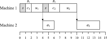
Optimal schedule with g(2,2,2,2,0)=20
-

Rights and permissions
About this article
Cite this article
Hwang, F.J., Kovalyov, M.Y. & Lin, B.M.T. Scheduling for fabrication and assembly in a two-machine flowshop with a fixed job sequence. Ann Oper Res 217, 263–279 (2014). https://doi.org/10.1007/s10479-014-1531-8
Published:
Issue Date:
DOI: https://doi.org/10.1007/s10479-014-1531-8