Enumeration of weighted games with minimum and an analysis of voting power for bipartite complete games with minimum

Abstract

This paper is a twofold contribution. First, it contributes to the problem of enumerating some classes of simple games and in particular provides the number of weighted games with minimum and the number of weighted games for the dual class as well. Second, we focus on the special case of bipartite complete games with minimum, and we compare and rank these games according to the behavior of some efficient power indices of players of type 1 (or of type 2). The main result of this second part establishes all allowable rankings of these games when the Shapley-Shubik power index is used on players of type 1.

1 Introduction

The study of voting systems can be traced back to the late nineteenth century, when Dedekind studied monotonic Boolean functions. In the context of voting systems these functions correspond to simple games. In their seminal book, Von Neumann and Morgenstern (1944) came up with the definition of a simple game as a type of cooperative game where the payoffs to coalitions are either 1 or 0, i.e., coalitions can be considered either winning or losing.

A particular case of simple games, and possibly the most important subcase, is that of weighted games, in which weights are assigned to players and a threshold is set so that a coalition is winning if and only if the sum of weights of its players is at least the threshold. This is natural in Parliaments and also in corporate voting when different shareholders may own different numbers of shares. Two natural extensions of weighted games have also been thoroughly studied: (1) complete games and (2) simple games with small dimension. In this paper we deal with a particular class of complete games, the so called “complete games with minimum” (see, e.g., Freixas and Puente 1998, 2008).

It turns out that every complete game with five or fewer players is weighted, so the smallest possible illustrations of complete non-weighted games occur for six players: y ₁, y ₂, b ₁, b ₂, b ₃, and b ₄ (here y means players of yellow type, whereas b means players of blue type), and we declare that a coalition is winning if and only if it contains: at least three players and at least one of them is yellow. Intuitively, it is clear that all the yellow players have the same influence (according to the desirability relation), and all the blue players have the same influence, but the yellow players have more influence than the blue players—suggesting a complete (weak) ordering for the players in this example of a voting system. In terms of the language we introduce later (in Sect. 2) this simple game is complete but not weighted.

Note that e.g., the coalitions of type {y ₁,y ₂,b _i } for i=1,2,3,4 are minimal winning since all players contained are essential for the coalition to be winning. The same occurs for the coalitions {y _i ,b _j ,b _k } for i=1,2 and 1≤j<k≤4. However, this latter set of coalitions has an additional singularity: none of the players in these coalitions can be replaced by a weaker player. E.g., we cannot replace in these coalitions the yellow player for a blue player since the new coalition obtained would not be winning. In terms of the language we introduce later (in Sect. 2) we say that the coalitions of type {y _i ,b _j ,b _k } for i=1,2 and 1≤j<k≤4 are shift-minimal winning coalitions. On the contrary, if in a shift-minimal winning coalition we replace a weaker player by a stronger one we obtain a minimal, but not shift-minimal, winning coalition. Finally, observe that all shift-minimal winning coalitions have the same number of players of each color, i.e., they all contain one yellow player and two blue players and this information can be encapsulated in the vector: (1,2) where the first component represents the number of yellow players and the second the number of blue players. Then, we refer to the game as being complete with only one type of shift-minimal winning coalitions, or equivalently, a complete game with minimum as was denominated in Freixas and Puente (1998, 2008). Note that in the previous example there is a bipartition between types of players: yellow players and blue players. Hence, the example introduced is a bipartite complete game with minimum.

The first part of the paper deals with enumerations for weighted games with minimum, while the second part deals with rankings of players for power indices in bipartite complete games with minimum. The dimension of complete games with minimum is studied in Freixas and Puente (2008). For instance, the previous example has dimension 2 and, therefore, it decomposes as the intersection of two weighted games: [5;3,3,1,1,1,1]∩[3;1,1,1,1,1,1] (the notation for a representation of a weighted game is introduced in the preliminaries section). Most existing voting systems have a small dimension. E.g., the current voting system of the European Council is an example of a complete game with dimension 3, i.e., it decomposes as an intersection of three weighted games which cannot be simplified to an intersection of fewer weighted games (Freixas 2004).

The voting system to amend the Canadian Constitution is an example of a non-weighted game which meets both requirements: it is complete (and has only one type of shift-minimal winning coalitions) and has dimension 2, i.e., it decomposes as the intersection of two weighted games. Since 1982, an amendment to the Canadian Constitution can become law only if it is approved by at least seven of the ten Canadian provinces, subject to the proviso that the approving provinces have, among them, at least half of Canada’s population. It was first studied in Kilgour (1983). A census (in percentages) taken from 1960 for the Canadian provinces was: Prince Edward Island (1 %), Newfoundland (3 %), New Brunswick (3 %), Nova Scotia (4 %), Manitoba (5 %), Saskatchewan (5 %), Alberta (7 %), British Columbia (9 %), Quebec (29 %) and Ontario (34 %). This is another example of a bipartite complete game with minimum and the vector representing all shift-minimal winning coalitions is: (1,6) where the first component indicates that exactly one of the two most populated provinces votes in favor of the voted law and 6-out-of-8 of the other provinces vote in favor of the voted law as well. Games of this type are the object of study in this paper.

This paper primarily concerns enumerations. The number of complete games is known up to nine players only (Freixas and Molinero 2010), and the number of weighted games is also known up to nine players (Kurz 2012). A seminal result on enumeration formulas for weighted games and complete games is May’s theorem (May 1952), and many other results have followed, e.g., the enumeration of weighted games with up to six players dates back at least to 1962 (Muroga et al. 1962).

The mathematical structure of complete games was studied in detail in the nineties by several scholars, e.g., in Krohn and Sudhölter (1995) and Carreras and Freixas (1996). In the latter work a system of quantities (called characteristic invariants) is associated with every complete game and their basic properties are stated. It is shown that these quantities determine the game (uniqueness) and that every such system is associated with some complete game (existence).

According to this classification the simplest case arises when the matrix (one of the two components of the characteristic invariants) has only one shift-minimal winning vector (which corresponds therefore to a set of closely related shift-minimal winning coalitions that are enough to generate the complete game). These games have been studied in Freixas (1997) and Freixas and Puente (1998). The first paper provides necessary and sufficient conditions to determine whether a game of this type is weighted. In the second paper the characteristic invariants are used to ease the calculus of different types of solutions of the game like the nucleolus, the kernel and semivalues.

The interest for this type of structures has also emerged in the field of Cryptography. The access structure in a secret sharing scheme (see e.g., Stinson 1992) can also be modeled by a simple game. To this end Simmons (1990) introduced the concept of a hierarchical access structure. Such an access structure stipulates that agents are partitioned into m levels, and a sequence of thresholds k ₁<k ₂<⋯<k _m is set, so that a coalition is authorized if and only if it has k ₁ agents of the first level and k ₂ agents of the first two levels and k ₃ agents of the first three levels etc. These hierarchical structures are called conjunctive since all the m conditions must be satisfied for a coalition to be authorized. If only one of the m conditions must be satisfied for a coalition to be authorized, then the structure is called disjunctive. A typical example of a conjunctive hierarchical game would be the United Nations Security Council, where for the passage of a resolution all five permanent members must vote for it and also at least nine members in total. The ideality of disjunctive games was proved by Brickell (1989), while the ideality of conjunctive games was proved by Tassa (2007). Ideality means they can carry the most informationally efficient secret sharing scheme and be completely secure (i.e., not giving any information about the secret to unauthorized coalitions). Gvozdeva et al. (2013) relate these two types of structures with complete games with one shift-minimal winning vector and with complete games with one-shift maximal losing vector.

In this paper we use game theoretic methods and terminology, and we talk about complete games with minimum or, equivalently, complete games with a unique shift-minimal winning vector (instead of hierarchical conjunctive structures) and games with a unique shift-maximal losing vector (instead of hierarchical disjunctive structures).

Here we enumerate weighted games with minimum. We find a polynomial formula as a function of the number of players of the game. This complements the corresponding known result for the enumeration of complete games of this type (Freixas and Puente 1998).

As for the second contribution, we recall that the distribution of power in some important real-world institutions (the International Monetary Fund, the voting system of the World Bank, the United Nations Security Council, the procedure to amend the Canadian Constitution, etc.) has been extensively studied, e.g., in Leech (2002a, 2002b), Alonso-Meijide and Bowles (2005), Taylor and Pacelli (2008), Felsenthal and Machover (1998), Straffin (1982) and Kilgour (1983) to cite just some references.

We consider here the set of bipartite complete games with minimum, i.e., complete games with two types of equivalent players and one shift-minimal winning vector, and discuss the possible rankings of these games given by the Shapley-Shubik power index for a player of type 1. The main result of this part establishes all the allowable rankings for the power of players of a given type in bipartite complete games with minimum for which the number of players of each type is fixed. We do remark that many papers in the literature have been devoted to study whether two or more power indices provide the same rankings in each game (see e.g., Diffo Lambo and Moulen 2002; Carreras and Freixas 2008; Freixas 2010). However, as far as we know, very little has been done on comparing power of players in different games.

The paper is organized as follows. In Sect. 2 we review some basic concepts and definitions of simple games, revise the terminology of the characteristic invariants for complete games and recall the known enumerations for complete games and for weighted games. In Sect. 3 we obtain a formula for the number of weighted games with one shift-minimal winning vector and deduce some consequences. In Sect. 4 we do a comparison of power for different complete games with two types of equivalent players and one shift-minimal winning vector. We prove that a limited number of rankings are possible for the Shapley-Shubik power index and we formulate a similar conjecture for the relative Banzhaf index. A study of duality in Sect. 5 permits us to extend the results obtained in the two previous sections to complete games with one shift-maximal losing vector. Some hints for future research are given in Sect. 6.

2 Preliminaries

This preliminary section is organized into five subsections. The first two refer to simple games in general and complete games in particular. The remaining three recall a result on the structure of complete games that will be essential for our purposes, previous results found in the literature on enumerations of games, and some power indices.

2.1 Simple games

A (monotonic) simple game is a pair $(N,\mathcal{W})$ where N={1,2,…,n} and $\mathcal{W}$ is a collection of subsets of N such that:

• (i) $\emptyset\notin\mathcal{W}$,

• (ii) $N \in\mathcal{W}$,

• (iii) if $S\in\mathcal{W}$ and S⊆T, then $T\in\mathcal{W}$.

From now on we will omit the term monotonic. Simple games can be viewed as models of voting systems in which a single alternative, such as a bill or an amendment, is pitted against the status quo. The set N is called the grand coalition, its members are called players and its subsets coalitions, and the subsets in $\mathcal{W}$ are called winning coalitions. The intuition here is that a set S is a winning coalition if and only if the bill or amendment passes when the players in S are precisely the ones who vote for it. A subset of N that is not in $\mathcal{W}$ is called a losing coalition and the collection of losing coalitions is denoted by ${\mathcal{L}}$. If each proper subcoalition of a winning coalition is losing, this winning coalition is called minimal. The set of minimal winning coalitions is denoted by $\mathcal{W}^{m}$. It should be noted that a simple game is completely determined by its minimal winning coalitions. If each proper coalition containing a losing coalition is winning, this losing coalition is called maximal. The set of maximal losing coalitions is denoted by ${\mathcal{L}}^{M}$ and it also determines the game.

Let $(N,\mathcal{W})$ be a simple game. The dual game of $(N, \mathcal{W})$ is the game $(N, \mathcal{W}^{\ast})$ where $\mathcal{W}^{\ast} = \{ S \subseteq N : N \setminus S \notin \mathcal{W} \}$.

A player i has veto in a simple game $(N,\mathcal{W})$ if $S\in \mathcal{W}$ implies i∈S. A player i∈N is called a null player in $(N,\mathcal{W})$ if i∉S for every $S\in\mathcal{W}^{m}$. A player i∈N is a dictator if and only if $\mathcal{W}^{m} = \{\{i\}\}$, in which case the remaining players in N become null players. Note that a dictator is the most extreme form of having veto.

A simple game $(N,\mathcal{W})$ is a weighted game if it admits a representation by means of n non-negative real numbers w ₁,…,w _n and a positive real number q such that $S\in \mathcal{W}$ if and only if w(S)≥q, where w(S)=∑ _i∈S w _i for each coalition S⊆N. The number q is called the quota of the game and w _i the weight of player i. From now [q;w ₁,…,w _n ] will mean the representation of $(N,\mathcal{W})$ by means of weights w ₁,…,w _n and quota q. The weighted representation (whenever it exists) is never unique. For instance, [c⋅q;c⋅w ₁,…,c⋅w _n ] is also a representation of $(N,\mathcal{W})$ for all c>0.

Two simple games $(N,\mathcal{W})$ and $(N^{\prime},\mathcal {W}^{\prime})$ are said to be isomorphic if there exists a bijective map f:N→N′ such that $S\in\mathcal{W}$ if and only if $f(S)\in \mathcal{W}^{\prime}$.

Let $(N,\mathcal{W})$ be a simple game. Set $\mathcal{W}_{i}=\{S\in \mathcal{W}:i\in S\}$ and let τ _ij :N→N denote the transposition of players i,j∈N (i.e., τ _ij (i)=j, τ _ij (j)=i and τ _ij (k)=k for k≠i,j). The individual desirability relation, introduced by Isbell (1956, 1958) and later generalized by Maschler and Peleg (1966), is the binary relation ≿ on N:

$$i \succsim j \quad \mbox{if and only if}\quad \tau_{ij}(\mathcal {W}_{j})\subseteq \mathcal{W}_{i}, $$

meaning that i is at least as desirable as j as a coalition partner. It is easy to see that ≿ is a preorder (i.e., a reflexive and transitive relation), we abbreviate i≿j, j≿i by i≈j and say that i and j are equi-desirable players (≈ is an equivalence relation in N), and we abbreviate i≿j, $j \not\succsim i$ by i≻j and say that i is strictly more desirable than j as a coalition partner.

The relation ≿ induces an ordering ≥ in the set of ≈-classes N/≈={N ₁,…,N _t }. Thus, N _p ≥N _q if and only if i≿j for any i∈N _p and any j∈N _q .

2.2 Complete games

The desirability is not always complete (total). Then, if any two players are comparable by ≿, $(N,\mathcal{W})$ is said to be a complete game;¹ in this case, the ≈-classes are linearly ordered by ≥. We say that a complete game has trivial classes if it possesses either veto or null players. Notice that each weighted game is complete because w _i ≥w _j implies i≿j.

A coalition $S \in\mathcal{W}$ is shift-minimal winning if $(S \setminus\{i\}) \cup\{j\} \notin\mathcal{W}$ for all i∈S and j∉S with i≻j. Note that a winning coalition can be minimal without being shift-minimal.

Example 2.1

Let $(N, \mathcal{W})$ be the simple game defined by N={1,2,3,4,5}, and $\mathcal{W}^{m} = \{ S \subseteq N :|S|=3, \ S \neq\{ 3,4,5\} \}$. It is easy to check that N decomposes into a bipartition of equivalent players N ₁={1,2} and N ₂={3,4,5}, and i≻j for all i∈N ₁ and j∈N ₂. Coalitions {1,2,3}, {1,2,4}, {1,2,5} are minimal winning but not shift-minimal winning in $(N, \mathcal{W})$. The remaining six winning coalitions of cardinality 3 are shift-minimal winning.

From now on we only deal with complete games and without loss of generality we assume 1≿2≿⋯≿n in the following. We can partition the whole set N of players into equivalence classes N ₁,…,N _t and say that the complete game consists of t types of (weakly) ordered players. By n _i we denote the cardinality of the set N _i for 1≤i≤t. Coalitions are categorized into different types, which can be described by a vector (m ₁,…,m _t ) meaning m _i -out-of-n _i players (from the set N _i ) for 1≤i≤t.

Let us consider Example 2.1 with n ₁=2 and n ₂=3. Due to the assumed ordering of the players we have N ₁={1,2} and N ₂={3,4,5} and i≻j for all i=1,2 and j=3,4,5 so that we can write N ₁>N ₂. With this, the vector (1,2) is the type of coalitions {1,3,4}, {1,3,5}, {1,4,5}, {2,3,4}, {2,3,5} and {2,4,5}. Since we have 1≈2 and 3≈4≈5 either all these six coalitions are winning or they are all losing and we can therefore speak of a winning or a losing vector. In Example 2.1 (1,2) is a (shift-minimal) winning vector.

Let $(N,\mathcal{W})$ be a simple game and N _h be the classes of equally desirable players for 1≤h≤t. We call a vector $\widetilde{m}:=(m_{1},\dots,m_{t})$, where 0≤m _h ≤|N _h | for 1≤h≤t, a winning vector if $S \in\mathcal{W}$, where S is an arbitrary coalition of N containing exactly m _h elements of N _h for 1≤h≤t. Analogously, we call such a vector a losing vector if $S \in\mathcal{L}$, where S is an arbitrary coalition of N containing exactly m _h elements of N _h for 1≤h≤t.

Following Carreras and Freixas (1996), several concepts of ordering among vectors (i.e., types of coalitions) in $\mathbb{N}_{0}^{t}$ (where $\mathbb{N}_{0}=\mathbb{N} \cup\{0\}$) have to be considered. For two vectors $\widetilde{a}=(a_{1},\dots,a_{t}) \in \mathbb{N}_{0}^{t}$ and $\widetilde{b} =(b_{1},\dots,b_{t}) \in\mathbb {N}_{0}^{t}$, representing types of coalitions in a complete simple game, we write (the standard componentwise order between vectors) $\widetilde{a} \geq\widetilde{b}$ if and only if we have a _i ≥b _i for all i=1,…,t. We use $\widetilde{a} > \widetilde {b}$ if $\widetilde{a} \geq\widetilde{b}$ and $\widetilde{a} \neq \widetilde{b}$. We write $\widetilde{a} \succeq\widetilde{b}$ if and only if we have $\sum_{i=1}^{k} a_{i} \geq\sum_{i=1}^{k} b_{i}$ for all 1≤k≤t. For $\widetilde{a} \succeq \widetilde{b}$ and $\widetilde{a} \neq\widetilde{b}$ we use $\widetilde{a} \succ\widetilde{b}$ as an abbreviation and say that they are comparable vectors with vector $\widetilde{b}$ being smaller than vector $\widetilde{a}$. If neither $\widetilde{a} \succeq \widetilde{b}$ nor $\widetilde{b} \succeq\widetilde{a}$ holds, we write $\widetilde{a} \bowtie\widetilde{b}$ and say that vector $\widetilde{a}$ and vector $\widetilde{b}$ are incomparable.

As (1,2) is a winning vector in Example 2.1, so are (1,3), (2,2) and (2,3) because of the monotonicity property required in the definition of simple game, but also is (2,1) because Example 2.1 is a complete game. From (1,2) nothing can be deduced about the vectors (1,1), (0,3), (0,2), (1,0) and (0,1). However, we can check that all the coalitions associated with these vectors are losing for Example 2.1.

A vector $\widetilde{m}=(m_{1},\dots,m_{t})$ in a complete game with t types of equivalent players $(N, \mathcal{W})$ is a minimal winning vector if $\widetilde{m}$ is a winning vector and every vector $\widetilde {m}'$ with $\widetilde{m}' < \widetilde{m}$ is losing. Analogously, a vector $\widetilde{m}$ is a maximal losing vector if $\widetilde{m}$ is a losing vector and every vector $\widetilde{m}'$ with $\widetilde{m}' > \widetilde{m}$ is winning. Of course, a vector is shift-minimal winning (resp., shift-maximal losing) if and only if any coalition represented by the vector is shift-minimal winning (resp., shift-maximal losing).

Similarly, a shift-minimal winning vector ² $\widetilde {m}$ is a winning vector such that every vector $\widetilde{m}'$ with $\widetilde{m}' \prec\widetilde{m}$ is losing. Analogously, a vector $\widetilde{m}$ is a shift-maximal losing vector if $\widetilde{m}$ is a losing vector and every vector $\widetilde{m}'$ with $\widetilde{m}' \succ\widetilde{m}$ is winning.

We denote by W ^m, W ^sm, L ^M and L ^sM the sets of minimal winning vectors, shift-minimal winning vectors, maximal losing vectors and shift-maximal losing vectors, respectively. In Example 2.1 we have:

The Hasse diagram for the ordering of vectors in complete games with the given hierarchy $\widetilde{n} =(2,3)$ is shown in Fig. 1.

Fig. 1

The Hasse diagram for the ordering ⪰ of vectors on $\widetilde{n} = (2,3)$

2.3 A parameterization theorem for complete games

Carreras and Freixas have given a full parameterization of complete games, up to isomorphisms, in Carreras and Freixas (1996) using vectors as models of coalitions and the partial order ⪰. We denote the (decreasing) lexicographic order by ⋗, i.e., we have (a ₁,…,a _n )⋗(b ₁,…,b _n ) if there is an index 1≤h≤n with a _i =b _i for all 1≤i<h and a _h >b _h . An example is given by (1,2,1)⋗(1,1,3).

Theorem 2.2

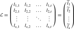
• (a) Assume that a vector $\widetilde{n} = (n_{1},n_{2}, \dots, n_{t})$ with natural coefficients and a matrix

  

  with natural or null coefficients are given, satisfying the following properties:

  • (i) m _1,1>0 and 0≤m _i,j ≤n _j , $m_{i,j}\in{\mathbb {N}_{0}}$ for 1≤i≤r and 1≤j≤t,

  • (ii) $\widetilde{m}_{i}\bowtie\widetilde{m}_{j}$ for all 1≤i<j≤r,

  • (iii) for each 1≤j<t there is at least one row-index i such that m _i,j >0, m _i,j+1<n _j+1, and

  • (iv) $\widetilde{m}_{i}\gtrdot\widetilde{m}_{i+1}$ for 1≤i<r.

  Then, there exists a unique complete game $(N, \mathcal{W})$ with invariants $(\widetilde{n},\mathcal{M} )$, i.e., with $\widetilde{n}$ as a vector of the cardinalities of the equivalence classes and matrix $\mathcal{M}$ where their rows consist of the shift-minimal winning vectors.

• (b) Two complete games $(N_{1},\mathcal{W}_{1} )$ and $(N_{2},\mathcal{W}_{2} )$ are isomorphic if and only if $\widetilde{n}_{1}=\widetilde{n}_{2}$ and $\mathcal{M}_{1}=\mathcal{M}_{2}$.

As a consequence of this theorem, any complete game can be denoted as $(\widetilde{n}, \mathcal{M})$, the pair of characteristic invariants of the game.

In such a vector/matrix representation (characteristic invariants) of a complete game the number of players n is determined by $n=\sum _{i=1}^{t} n_{i}$. Although Theorem 2.2 looks technical at first glance, the necessity of the required properties is easily explained. Obviously, n _j ≥1 and 0≤m _i,j ≤n _j must hold for 1≤i≤r, 1≤j≤t. If $\widetilde{m}_{i}\preceq\widetilde{m}_{j}$ or $\widetilde{m}_{i}\succeq\widetilde{m}_{j}$ then we have $\widetilde {m}_{i}=\widetilde{m}_{j}$ or either $\widetilde{m}_{i}$ or $\widetilde{m}_{j}$ cannot be a shift-minimal winning vector. If for a column-index 1≤j<t we have m _i,j =0 or m _i,j+1=n _j+1 for all 1≤i≤r, then we can check whether we have g≈h for all g∈N _j , h∈N _j+1, which is a contradiction to the definition of the classes N _j and therefore also for the numbers n _j . Obviously a complete game does not change if two rows of the matrix $\mathcal{M}$ are interchanged. Thus we require a given ordering of the rows to avoid repetitions: ⋗ stands for the lexicographic ordering of vectors in $\mathbb{N}_{0}^{t}$.

As the desirability relation is total in complete games, it defines for these games a weak ordering on the set of players. For example, writing that a five-player complete game has hierarchy 1>2=3=4>5 means that there is one player which has the maximum influence, another one that has the minimum influence and the other three have all the same intermediate influence, in that case we can represent the previous ordering as the vector (1,3,1). We say that two complete games have the same hierarchy if the ordering that defines the desirability relation on them is the same. Thus, if $(\widetilde{n}_{1},\mathcal {M}_{1} )$ and $(\widetilde{n}_{2},\mathcal{M}_{2} )$ are the characteristic invariants of two complete games, they have the same hierarchy if $\widetilde{n}_{1} = \widetilde{n}_{2}$.

The Hasse diagram for the ordering ⪰ of vectors in complete games with the given hierarchy $\widetilde{n} =(2,2)$ is shown in next Fig. 2.

Fig. 2

The Hasse diagram for the ordering ⪰ of vectors on $\widetilde{n} = (2,2)$

We would like to remark that for t=1 only r=1 is possible and the requirements in Theorem 2.2 reduce to 1≤m _1,1≤n ₁=n. Also for t=2 one can easily give a more compact formulation for the requirements in Theorem 2.2. A complete description of the possible values n ₁, n ₂, m _1,1, m _1,2 corresponding to a complete game with parameters n, t=2, and r=1 is given by

Two important real-world examples of voting weighted games with only one shift-minimal winning vector are (see Chap. 8 in Taylor and Pacelli 2008 for more details on these two examples): the United Nations Security Council—without taking abstention into consideration—and the procedure to amend the Canadian Constitution. These examples have $(\widetilde{n}, {\mathcal{M}} ) = ((5,10),(5,4) )$ and $(\widetilde{n}, {\mathcal{M}} ) = ((2,8),(1,6) )$ as respective characteristic invariants.

2.4 Known enumerations for weighted games and for complete games

Let wg(n,t,r) be the number of weighted games with n players, t equivalence classes N ₁,…,N _t and r shift-minimal winning vectors. Let wg(n,∗,r)³ be the number of weighted games with n players and r shift-minimal winning vectors (independently of the number of equivalence classes, t). Let wg(n,t,∗) be the number of weighted games with n players, and t equivalence classes N ₁,…,N _t (independently of the number of shift-minimal winning vectors, r). We identify wg(n,∗,∗), i.e., the number of weighted games with n players independently of the values of r and t, with simply wg(n). Analogous notations cg(n,t,r), cg(n,∗,r), cg(n,t,∗) and cg(n) will be used for the respective enumerations of complete games.

The first exact counting can at least be traced back to May (1952) which establishes the number of symmetric or anonymous simple games. Any such game with n players admits a weighted representation $[q;\underbrace{1,1,\dots,1}_{n}]$ where q∈{1,…,n}.

Let wg ^sym(n), cg ^sym(n) and sg ^sym(n) be respectively the number of symmetric: weighted games, complete games and, simple games with n players.

Theorem 2.3

wg(n,1,1)=cg(n,1,1)=n=wg ^sym(n)=cg ^sym(n)=sg ^sym(n).

The number of complete games with one shift-minimal winning vector was determined in Freixas and Puente (1998), and a more refined result appears in Freixas and Puente (2008) (parts 1 and 2 of the next result respectively).

Theorem 2.4

• 1. cg(n,∗,1)=2ⁿ−1,

• 2.
  $$cg(n,t,1) = \left \{ \begin{array}{l@{\quad}l} n, & \mbox{\textit{if} } t=1, \\ [2pt] \binom{n+1}{2t-1}, & \mbox{\textit{if}} \ 2 \leq t \leq\frac{n}{2}+1, \\ [2pt] {0}, & \mbox{\textit{otherwise}}. \end{array} \right . $$

Other formulas have been obtained quite recently. In Freixas et al. (2012b) we can find the next enumeration, where F(n) are the Fibonacci numbers, which constitute a well-known sequence of integer numbers defined by the following recurrence relation: F(0)=0, F(1)=1, and F(n)=F(n−1)+F(n−2) for all n>1.

Theorem 2.5

cg(n,2,∗)=F(n+6)−(n ²+4n+8).

Let us finally remark that a formula for cg(n,∗,2) is found in Kurz and Tautenhahn (2012).

Theorem 2.6

In Kurz and Tautenhahn (2012) it is proved that cg(n,t,r) is a quasi-polynomial in n, if t and r are given, and can therefore be automatically computed (without escaping of the problem of capacity limitations). The main purpose of Sect. 3 is to determine wg(n,∗,1) as well as to obtain other related finer results.

2.5 Power indices

Informally a power index is a numerical measure that estimates the a priori capacity or influence of each player in a simple game. Of course the notion of power is complex and has been analyzed in depth by several authors. An interesting reference is the book by Morriss (2002), which analyzes power from a philosophical point of view.

Two prominent power indices are more recognized and used than others, and both known power indices, and both of them are based on the notion of a swing. A coalition S is a swing for i∈S if and only if $S \in\mathcal{W}$ but $S\setminus\{i\} \notin\mathcal{W}$. Let $c_{i}(N, \mathcal{W})$ denote the number of swings of player i in game $(N, \mathcal{W})$. Then the relative Banzhaf index (Banzhaf 1965) is defined as

$$Bz_i(N, \mathcal{W}) = \dfrac{c_i(N,\mathcal{W})}{\sum_{j \in N} c_j(N,\mathcal{W})} $$

while the absolute Banzhaf index (Owen 1978) is defined as

$$Bz_i'(N, \mathcal{W}) = \frac{c_i(N,\mathcal{W})}{2^{n-1}}. $$

The Shapley-Shubik index (Shapley and Shubik 1954), which is the restriction of the well-known Shapley (1953) value for cooperative games, can be expressed as a function of the swings as follows. Let s be the cardinality of the swing S for i and $c_{i}^{s}(N, \mathcal{W})$ be the number of swings for i for coalitions S of cardinality s. Then,

$$SS_i(N, \mathcal{W}) = \sum_{s=1}^n \frac{(s-1)!(n-s)!}{n!} c_i^s(N, \mathcal{W}). $$

This less usual formulation of the Shapley-Shubik index will be helpful here for our purposes. The Shapley-Shubik index of a player can be viewed as his/her expected part of a fixed total prize, i.e., the power of a player is meant to be the player’s expected payoff. Dubey and Shapley (1979) proved the following result.

Proposition 2.7

If $(N, \mathcal{W})$ is any simple game then, for all i∈N, we have

• (a) $SS_{i}(N, \mathcal{W}) = SS_{i}(N, \mathcal{W}^{\ast})$.

• (b) $Bz_{i}(N, \mathcal{W}) = Bz_{i}(N, \mathcal{W}^{\ast})$ and $Bz'_{i}(N, \mathcal{W}) = Bz'_{i}(N, \mathcal{W}^{\ast})$.

The fact that $c_{i}^{s}(N,\mathcal{W}) = c_{i}^{s}(N,\mathcal{W}^{\ast})$ for all s=1,2,…,n justifies (a) and implies that $c_{i}(N, \mathcal{W})=c_{i}(N,\mathcal{W}^{\ast})$, which justifies (b), a property discovered by Dubey and Shapley (1979).

3 Counting weighted games with minimum

If we consider a subgame of a weighted game when this game is stripped of its null and veto players, then the original game is weighted if and only if the subgame is weighted and, similarly, the original game is complete if and only if the subgame is complete, see e.g., Taylor and Zwicker (1999).

Let $(\widetilde{n},\mathcal{M} )$ be a complete game with t equivalence classes. By $(\widetilde{n},\mathcal{M} ){\downarrow}$ we denote

where s=1 if there are no veto players, s=2 if there are veto players (which would form the strongest class), e=t if there are no null players, and e=t−1 if there are null players (which would form the weakest class). If all players of $(\widetilde{n},\mathcal {M} )$ have veto or are null players $(\widetilde{n},\mathcal {M} ){\downarrow}$ is empty.

For instance, $(\widetilde{n},\mathcal{M} ){\downarrow}$ does not change for the system to amend the Canadian Constitution, i.e., $(\widetilde{n},\mathcal{M} ){\downarrow}= (\widetilde{n},\mathcal{M} ) = ( (2,8), (1 \ 6) )$, whereas $(\widetilde{n},\mathcal{M} ) {\downarrow}$ reduces to ((10),(4)) for the United Nations Security Council, because the five permanent members have veto right.

Lemma 3.1

Let $\widehat{wg}(n,t,r)$ be the number of non-trivial weighted games with t equivalence classes N ₁,…,N _t and r shift-minimal winning vectors. For r>1 or t>2 we have

$$ \begin{aligned}[b] wg(n,t,r)=&\widehat{wg}(n,t,r)+ \sum_{h=1}^{n-1} 2\cdot\widehat {wg}(n-h,t-1,r) \\ &{}+(h-1)\cdot\widehat{wg}(n-h,t-2,r), \end{aligned} $$

(1)

where we define $\widehat{wg}(n,t,r)=0$ for the non-feasible cases n<t or t<1. For r=1 and t=1 an additional 1 has to be added to the right hand side of Eq. (1), and for r=1 and t=2 an additional term n−1 has to be added to the right hand side of Eq. (1).

Proof

Every weighted game arises from a non-trivial weighted game or an empty game by appending h ₁≥0 veto players and h ₂≥0 null players. □

For r=1 and arbitrary t the set of maximal losing vectors of complete games without null players, i.e., with m _1,t ≥1, was analytically given in Freixas and Puente (2008) (see next lemma). As for r=1 the first indices in vector $\widetilde{m}_{1}$ do not carry any information we omit them.

Lemma 3.2

For a complete game

$$\bigl( (n_1,\dots,n_t) ,(m_{1} \dots m_{t}) \bigr) $$

without null players, i.e., with m _t ≥1, the complete set of shift-maximal losing vectors is given in the following matrix:

where

$$a_{i,j}:=\max \Biggl\{0,\min \Biggl\{n_j,\,-1+\sum _{h=1}^i m_{h}-\sum _{h=1}^{j-1}n_h \Biggr\} \Biggr\} $$

for 1≤j≤i≤t.

Note that each vector $\widetilde{a}_{i}$ for 1≤i≤t represents shift-maximal losing coalitions. Indeed, these coalitions contain $\sum_{j=1}^{i} m_{j}-1$ strongest players (according to the desirability relation) and additionally they also contain the $\sum_{j=i+1}^{t} n_{j}$ weakest players, i.e., those players that belong to the t−i weakest equivalence classes, from the (i+1)th class to the tth last class. If in one of these coalitions an additional player was added or a weaker player was replaced by a stronger one, then the new vector $\widetilde{b}$ representing the coalition would contain at least $\sum_{j=1}^{i} m_{j}$ players for each 1≤i≤t and therefore would be winning.

The conditions (i)–(iv) of Theorem 2.2(a) reduce to 1≤m ₁≤n ₁, 0≤m _t ≤n _t −1, and 1≤m _h ≤n _h −1 for all h such that 2≤h≤t−1. We remark that if a complete game with r=1 has null players, then the complete set of shift-maximal losing vectors is given by the vectors in Lemma 3.2 except for the last vector $\widetilde{a}_{t}$. We would like to remark too that $\widetilde{a}_{t}$ is a losing vector which is not maximal and that there is a typo in the remark of Freixas and Puente (2008), i.e., the first row (instead of the last one) must be deleted.

Having an analytic description of the shift-maximal losing vectors at hand it is not too hard to characterize the set of weighted games analytically. Indeed, already in Freixas (1997) the non-trivial weighted games with r=1, i.e., those having exactly one shift-minimal winning vector, were completely classified.

Theorem 3.3

A non-trivial complete game $(\widetilde{n},\mathcal{M} )$ with r=1 is a weighted game if and only if either t=1 or t=2 and m ₂∈{1,n ₂−1}.

Proof

Due to Theorem 2.2 we can assume t≥2. For t=2 the shift-maximal losing vectors are given by

$$(m_{1}-1, n_2) \quad\mbox{and}\quad(m_{1}+c, m_{2}-1-c), $$

where c=min(n ₁−m ₁,m ₂−1). Choosing w ₁=1 we conclude

which is equivalent to $w_{2}<\frac{1}{n_{2}-m_{2}}$ and (1+c)w ₂>c. If m ₂=n ₂−1 or c=0, which is equivalent to m ₂=1, there exists a solution for w ₂. If m ₂≤n ₂−2 and c≥1 the two inequalities are contradicting.

Now we consider the remaining cases t≥3. Here the vectors

$$(m_{1}-1,n_2,\dots,n_t ), \quad\mbox{and} \quad (m_{1}+1,m_{2}-1,m_{3}-1,n_4, \dots,n_t) $$

are losing vectors (the second not necessarily shift-maximal). Thus for w ₁=1 we have

from which we conclude 1>w ₂+w ₃ and w ₂+w ₃>1, which is a contradiction. □

Thus together with Lemma 3.1 and Theorem 2.3 we can conclude:

Theorem 3.4

For n≥1 we have

Adding up the previous enumerations we get the following compact expression for the total number of weighted games with a unique shift-minimal winning vector.

Corollary 3.5

$$wg(n,\ast,1) = \left \{ \begin{array}{l@{\quad}l} 2^n-1 & \mbox{\textit{if}} \ n \leq5, \\ \frac{n^4-6n^3+23n^2-18n+12}{12} & \mbox{\textit{if}} \ n \geq6. \end{array} \right . $$

Thus, the numbers of weighted games wg(n,∗,1) and complete games cg(n,∗,1) (see Theorem 2.4) coincide for n≤5 players, but their ratio converges to zero as n increases. An asymptotic upper bound for weighted games is given in de Keijzer et al. (2010) and an asymptotic lower bound for complete games is given in Peled and Simeone (1985), where these games are called regular Boolean functions. Many useful and accurate asymptotic estimations for simple games and subclasses of them are provided in Korshunov (2003).

4 Analysis of voting power for bipartite complete games with minimum

Many papers have been devoted to study classes of games for which two or more power indices provide the same rankings in every game of such classes, see e.g., Diffo Lambo and Moulen (2002), Carreras and Freixas (2008), Freixas (2010). However, as far as we know, very little has been studied about comparisons of different games depending on how a given power index acts on them.

In this section we will consider complete games with two types of equivalent players and with only one shift-minimal winning vector. For these games we will give explicit formulas to calculate some efficient power indices. Since the games have only two types of equivalent players and the considered power indices are efficient, it will be possible to totally rank these games according to the behavior of the power index on players that belong to a fixed class. Of course, the order obtained considering the power over a type of players for bipartite complete games with games with minimum is reversed if the power index is evaluated over players that belong to the other equivalence class.

An important tool to this purpose is monotonicity in Young’s (1985) sense which was used to give a characterization of the Shapley value that avoids additivity. If we assume a fixed set of players N we write $\mathcal{W} B_{i} \mathcal{W}'$ whenever if S is a swing for i in $\mathcal{W}'$ then S is a swing for i in $\mathcal{W}$. Relation B _i allows us to qualitatively compare the position of a given player i in two games. However, we do not see a direct application of such a monotonicity for most of the cases we are going to study.

4.1 Allowable rankings for the Shapley-Shubik index

The main purpose of this subsection is to study the allowable hierarchies that the Shapley-Shubik index produces when applied to different bipartite complete (t=2) games with minimum (r=1). We also illustrate the difficulty to extend similar results for other power indices.

Proposition 4.1

Let $(\widetilde{n},\mathcal{M} )$ be a complete game with $\widetilde{n}=(n_{1},n_{2})$ and $\mathcal{M}= (a\ b)$, where a≥1 and b≤n ₂−1.

• (1) For a player of type 1 the number of coalitions where he is a swing player is given by

  $$c_1=\sum_{i=b+1}^{n_2} \binom{n_1-1}{a-1}\cdot \binom{n_2}{ i}+ \sum _{i=0}^{\min\{b,n_1-a\}}\binom{n_1-1}{ a+i-1} \cdot\binom{n_2}{ b-i}. $$

• (2) For a player of type 2 the number of coalitions where he is a swing player is given by ⁴

  $$c_2=\sum_{i=0}^{\min\{b-1,n_1-a\}}\binom{n_1}{ a+i} \cdot \binom{n_2-1}{ b-i-1}. $$

• (3) The Shapley-Shubik power index SS ₁(a,b,n ₁,n ₂) of a player of type 1 is given by

  

• (4) The Shapley-Shubik power index SS ₂(a,b,n ₁,n ₂) of a player of type 2 is given by

  $$\frac{(a+b-1)!\cdot(n-a-b)!}{n!}\cdot\sum_{i=0}^{\min\{b-1,n_1-a\} }\binom{n_1}{ a+i}\cdot\binom{n_2-1}{ b-i-1}. $$

• (5) For b≥1 we have

  

• (6) For a≥2 we have

  

Proof

(1) The vectors representing coalitions where a player of type 1 is a swing player are given by (a,b+1), (a,b+2), … , (a,n ₂) and (a,b), (a+1,b−1), (a+2,b−2), …,(c,d) where:

$$(c,d) = \left \{ \begin{array}{l@{\quad}l} (a+b,0), & \mbox{if} \ a+b \leq n_1, \\ (n_1,a+b-n_1), & \mbox{otherwise}. \end{array} \right . $$

The number of swings for a player of type 1 for an arbitrary vector (x,y) is: ${\binom{n_{1}-1}{ x-1} \cdot\binom{n_{2}}{ y}}$.

(2) The vectors representing coalitions where a player of type 2 is a swing player are given by (a,b), (a+1,b−1), (a+2,b−2), … , (e,f) where:

$$(e,f) = \left \{ \begin{array}{l@{\quad}l} (a+b-1,1), & \mbox{if} \ a+b \leq n_1, \\ (n_1,a+b-n_1), & \mbox{otherwise}. \end{array} \right . $$

The number of swings for a player of type 2 for an arbitrary vector (x,y) with y>0 is: $\binom{n_{1}}{ x} \cdot\binom{n_{2}-1}{ y-1}$.

(3)–(4) These results follow from the definition given in this paper for the Shapley-Shubik index and parts (1)–(2) respectively. (5) For n ₁−a≤b−2 we have

and for n ₁−a≥b−1 we have:

both of which can be simplified to the stated expression.

(6) Similar to (5). □

Corollary 4.2

• 1. For a given vector (n ₁,n ₂) let ((m ₁,m ₂)) and $((m_{1}',m_{2}'))$ be two different complete simple games, i.e., $0<m_{1},m_{1}'\le n_{1}$ and $0\le m_{2},m_{2}'<n_{2}$. If $m_{1}\ge m_{1}'$ and $m_{2}\le m_{2}'$ then $SS_{2}(m_{1},m_{2}) \le SS_{2}(m_{1}',m_{2}')$ and $SS_{1}(m_{1},m_{2}) \ge SS_{1} (m_{1}',m_{2}')$, where equality holds if and only if $m_{2}=m_{2}'=0$.

• 2. For a given vector (n ₁,n ₂):

  $$ \frac{1}{n} <SS_1(1,n_2-1) \leq SS_1(m_1,m_2) \leq SS_1(n_1,1) < SS_1(c,0) = \frac{1}{n_1} $$

  (2)

  where c is any integer number between 1 and n ₁.

  Inequalities (2) imply

  $$\frac{1}{n} >SS_2(1,n_2-1) \geq SS_2(m_1,m_2) \geq SS_2(n_1,1) > SS_2(c,0) = 0 $$

  where c is any integer number between 1 and n ₁.

Remark 4.3

We have implemented a computer program which can determine the Banzhaf and the Shapley-Shubik power index for bipartite complete games with minimum. For the case n ₁=3, n ₂=7 we have the following ordering with respect to SS ₁:

Note that, in general, for an arbitrary pair (n ₁,n ₂) the rankings of some games with respect to SS ₁ or Bz ₁ (printed in bold in the previous example) are fixed. We refer to the games of type (c,0) for c>0 which are always tied among them and situated on the top of the ranking and, oppositely, the game (1,n ₂−1) which is always situated at the bottom of the ranking. These extreme games are highlighted in black in the previous example for n ₁=3, n ₂=7. Additionally, Corollary 4.2 provides some constraints on the rankings of the different games with respect to SS ₁ or Bz ₁:

• 1. leaving the first component fixed:

  (3,1)>(3,2)>(3,3)>(3,4)>(3,5)>(3,6);

  (2,1)>(2,2)>(2,3)>(2,4)>(2,5)>(2,6); and

  (1,1)>(1,2)>(1,3)>(1,4)>(1,5)>(1,6).

• 2. leaving the second component fixed:

  (3,1)>(2,1)>(1,1); (3,2)>(2,2)>(1,2); (3,3)>(2,3)>(1,3);

  (3,4)>(2,4)>(1,4); (3,5)>(2,5)>(1,5) and (3,6)>(2,6)>(1,6).

Taking into account all these restrictions we have that for the given hierarchy $\overline{n} = (3,7)$ we have 13 weighted games, three of which are of type (c,0) and give the maximum value 1/n ₁=1/3 for the SS ₁ to three most powerful players; the ranking of all other games with respect to SS ₁ is strict so that there are, in principle, 10! potential strict orderings for the power of SS ₁ over the set of these games, but Corollary 4.2 guarantees that at most 12 of these rankings are possible.

4.2 Comparisons for the two Banzhaf indices

As we shall see in this section, we find for the relative Banzhaf index a similar result to that one obtained for the Shapley-Shubik index (for less than 100 players), while it fails for the absolute Banzhaf index.

The relative Banzhaf power index Bz ₁(a,b,n ₁,n ₂) of a player of type 1 is given by

$$\frac{c_1}{n_1\cdot c_1+n_2\cdot c_2}. $$

The relative Banzhaf power index Bz ₂(a,b,n ₁,n ₂) of a player of type 2 is given by

$$\frac{c_2}{n_1\cdot c_1+n_2\cdot c_2}. $$

The absolute Banzhaf power index $Bz_{1}'(a,b,n_{1},n_{2})$ of a player of type 1 is given by

$$\frac{c_1}{2^{n-1}}. $$

The absolute Banzhaf power index $Bz_{2}'(a,b,n_{1},n_{2})$ of a player of type 2 is given by

$$\frac{c_2}{2^{n-1}}. $$

Remark 4.4

For the Banzhaf absolute power index, Corollary 4.2 is wrong, and an example is given by n=4, n ₁=n ₂=2 and the games ((2,1)), ((1,1)) with Banzhaf values $(\frac {3}{8},\frac{1}{8} )$, $(\frac{4}{8},\frac{2}{8} )$, respectively. Another example is given by n=7, n ₁=3, n ₂=4 and the games ((3,1)) and ((2,2)) with absolute Banzhaf indices $(\frac{15}{64},\frac {1}{64} )$, $(\frac{26}{64},\frac{10}{64} )$, respectively.

Example 4.5

(Ties)

Let us consider the equality case in Corollary 4.2 for the relative Banzhaf power index, i.e., where the powers sum up to 1. For $m_{2}=m_{2}'=0$ equality holds. Other examples are given by

• n=7, n ₁=3, and the games ((3,3)), ((1,2)) with Banzhaf numerators (5,3), (20,12),

• n=8, n ₁=2, and the games ((2,5)), ((1,4)) with Banzhaf numerators (7,5), (42,30),

• n=9, n ₁=6, and the games ((6,2)), ((1,1)) with Banzhaf numerators (4,2), (12,6),

• n=13, n ₁=5, and the games ((5,7)), ((2,5)) with Banzhaf numerators (9,7), (1044,812),

• n=13, n ₁=9, and the games ((6,2)), ((1,1)) with Banzhaf numerators (736,288), (23,9).

These are all examples where $(m_{1},m_{2})>(m_{1}',m_{2}')$ or $(m_{1},m_{2})<(m_{1}',m_{2}')$. If we assume $m_{1}\ge m_{1}'$ and $m_{2}\le m_{2}'$ then there is no further example for n≤32.

Remark 4.6

For the relative Banzhaf power index Corollary 4.2 is true for all n≤100.

This suggests to ask whether Corollary 4.2 is true for the relative Banzhaf index for all n.

Conjecture 4.7

• (1) For b≥1 we have Bz ₂(a,b,n ₁,n ₂)−Bz ₂(a,b−1,n ₁,n ₂)>0.

• (2) For a≥2 we have Bz ₂(a−1,b,n ₁,n ₂)−Bz ₂(a,b,n ₁,n ₂)≥0 which equals zero for b=0 and otherwise it is positive.

It would imply a corollary analogous to Corollary 4.2.

Corollary 4.8

• 1. For a given vector (n ₁,n ₂) let ((m ₁,m ₂)) and $((m_{1}',m_{2}'))$ be two different complete simple games, i.e., $0<m_{1},m_{1}'\le n_{1}$ and $0\le m_{2},m_{2}'<n_{2}$. If $m_{1}\ge m_{1}'$ and $m_{2}\le m_{2}'$ then $Bz_{2}(m_{1},m_{2}) \le Bz_{2}(m_{1}',m_{2}')$ and $Bz_{1}(m_{1},m_{2}) \ge Bz_{1} (m_{1}',m_{2}')$, where equality holds if and only if $m_{2}=m_{2}'=0$.

• 2. For a given vector (n ₁,n ₂):

  $$ \frac{1}{n} < Bz_1(1,n_2-1) \leq Bz_1(m_1,m_2) \leq Bz_1(n_1,1) < Bz_1(c,0) = \frac{1}{n_1} $$

  (3)

  where c is any integer number between 1 and n ₁.

  Inequalities (3) imply

  $$\frac{1}{n} >Bz_2(1,n_2-1) \geq Bz_2(m_1,m_2) \geq Bz_2(n_1,1) > Bz_2(c,0) = 0 $$

  where c is any integer number between 1 and n ₁.

However, the ranking over different games for Shapley-Shubik and relative Banzhaf index are not necessarily the same, as the following example illustrates.

Example 4.9

For the case n ₁=3, n ₂=7 we have checked the following rankings with respect to Bz ₁:

This ranking of different games with vector $\widetilde{n} = (3,7)$ does not coincide with the ranking obtained for the SS ₁ but, restricted to weighted games, it is one of the 12 expected rankings for the SS ₁ according to Corollary 4.2.

Remark 4.10

One might conjecture that Corollary 4.2 holds for some effective generalized power indices as for example semivalues. Semivalues for simple games (or power semiindices) are uniquely determined as those power indices that satisfy: symmetry, positivity, dummy player property and transfer (see Carreras et al. 2003) and with specific coefficients $\{p_{j}\}_{j=1}^{n}$ such that $\sum_{j=1}^{n} p_{j}\binom{n-1}{ j-1}=1$ and p _j ≥0 for all j. The absolute Banzhaf power index is given by p _j =1/2ⁿ⁻¹ for all 1≤j≤n and the Shapley-Shubik power index is given by $p_{j} = \frac{1}{n \binom{n-1}{ j-1}}$. The (unnormalized) power, SV, of player i is given by

$$SV(i):=\sum_{i=1}^n p_{|S|} \cdot c^s_i, $$

where |S|=s.

Let us consider the following example: n=10, n ₁=7, and the games ((7,1)) and ((1,2)) with power index numerators (3p ₇+3p ₈+p ₉,p ₇), (36p ₂+p ₃,35p ₂). This example is a counterexample to Corollary 4.8 if and only if

$$207p_2p_7+315p_2p_8+105p_2p_9-3p_3p_7<0. $$

If we assume p _j =p _n−j−1 then this is equivalent to

$$p_2\cdot (105p_0+325p_1+207p_2-3p_3 )<0, $$

and thus it is possible.

5 Results preserved by duality

This section establishes a simple but significant result on enumerations and highlights that the results obtained in the previous section about power indices are preserved by duality.

Let us recall that the dual game of $(N, \mathcal{W})$ is $(N, \mathcal{W}^{\ast})$ where: $\mathcal{W}^{\ast} = \{ S \subseteq N : N \setminus S \notin\nobreak \mathcal{W} \}$. Then it is not difficult to check the following:

Lemma 5.1

• (i) $(N, \mathcal{W})$ is weighted if and only if $(N, \mathcal{W}^{\ast})$ is weighted, and if [q;w ₁,…,w _n ] is an integer representation for $(N,\mathcal{W})$ then [T−q+1;w ₁,…,w _n ] is an integer representation for $(N,\mathcal{W}^{\ast})$ where $T = \sum_{i=1}^{n} w_{i}$ and vice versa.

• (ii) i≿j if and only if i≿^∗ j where ≿^∗ stands for the desirability relation for game $(N, \mathcal{W}^{\ast})$. Thus, $(N, \mathcal{W})$ is complete if and only if $(N, \mathcal{W}^{\ast})$ is complete, and the ≈-classes N _i for $(N, \mathcal{W})$ and its ordering N ₁>N ₂⋯>N _t are preserved by ≿^∗, i.e., $(N, \mathcal{W})$ and $(N, {\mathcal{W}}^{\ast})$ have the same ranking $\widetilde{n}$.

• (iii) The complete game $(N, \mathcal{W})$ has the vector $\widetilde{n}=(n_{1},\dots,n_{t})\in\mathbb{N}_{>0}^{t}$ and the matrix

  

  as characteristic invariants (hence, fulfilling properties (1)–(4) in Theorem 2.2) and matrix

  

  of shift-maximal losing vectors if and only if the complete game $(N, \mathcal{W}^{\ast})$ has vector $\widetilde{n}=(n_{1},\dots,n_{t})\in\mathbb {N}_{>0}^{t}$ and matrix

  

  as characteristic invariants (hence, fulfilling properties (1)–(4) in Theorem 2.2(a)) and matrix

  

  of shift-maximal losing vectors.

Let $\overline{cg}(n,t,r)$ be the number of complete games with n players, with t equivalence classes and r shift-maximal losing vectors and similar notation for: $\overline{cg}(n,\ast,r)$, $\overline {wg}(n,t,r)$ and $\overline{wg}(n,\ast,r)$. Lemma 5.1 allows us to deduce the next corollary and describes how the bijection for characteristic invariants works.

Corollary 5.2

${cg}(n,t,r) = \overline{cg}(n,t,r)$ and ${wg}(n,t,r) = \overline{wg}(n,t,r)$.

The application of this Corollary and the results on enumerations in Sects. 2 and 3 to games with one shift-maximal losing vector gives the enumerations for complete games and for weighted games respectively. An analogous version of Theorem 2.4 is given by

Corollary 5.3

• 1. $\overline{cg}(n,\ast,1)=2^{n}-1$,

• 2.
  $$\overline{cg}(n,t,1) = \left \{ \begin{array}{l@{\quad}l} n, & \mbox{\textit{if}} \ t=1, \\ \binom{n+1 }{2t-1}, & \mbox{\textit{if}} \ 2 \leq t \leq\frac{n}{2} + 1, \\ {0}, & \mbox{\textit{otherwise}} . \end{array} \right . $$

An analogous version of Corollary 3.5 is given by

Corollary 5.4

$$\overline{wg}(n,\ast,1) = \left \{ \begin{array}{l@{\quad}l} 2^n-1, & \mbox{\textit{if}} \ n \leq5, \\ \frac{n^4-6n^3+23n^2-18n+12}{12}, & \mbox{\textit{if}} \ n \geq6. \end{array} \right . $$

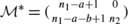
Due to Proposition 2.7 and Lemma 5.1 it follows that the results in Sect. 4 for the Shapley-Shubik index extend to complete games with one-shift maximal losing vector, since for any given (n ₁,n ₂) and $\mathcal{M} = (a \quad b)$, the dual game is given by the same vector and matrix $\mathcal{L}^{\ast} = (n_{1}-a \quad n_{2}-b)$ which corresponds to matrix $\mathcal{M}^{\ast}$ where:

• (i) $\mathcal{M}^{\ast} = (n_{1}-a+1 \quad 0)$ if b=0, otherwise:

• (ii) if a+b−1≤n ₁,

• (iii) if a+b−1>n ₁.

Thus Proposition 4.1 has a simple analogue, and therefore Corollary 4.2 has a simple analogue too. The conjecture stated for the relative Banzhaf index derived for the computation up to 100 players is also open in this dual context.

6 Future work

Any progress concerning enumeration of games, like cg(n,t,r) or wg(n,t,r), will be a significant advance in both directions: either providing new formulas or providing tighter bounds. In Kurz and Tautenhahn (2012) it is proved that cg(n,t,r) is a quasi-polynomial in n, if t and r are given, and can therefore be automatically computed (without escaping of the problem of capacity limitations). We wonder whether these automatic computations can be performed for the number wg(n,t,r) of weighted games.

We also encourage research in other classes of simple games. For instance, roughly weighted games (considered in Taylor and Zwicker 1999 and extensively studied in Gvozdeva and Slinko 2011) which are complete, i.e., roughly weighted complete games with n players and t types of equivalent players to determine rcg(n,t,r).

As a future research concerning Sect. 4 (and 5) it would be nice to find the proofs of our Conjectures 4.7 and 4.8. It seems likely that these conjectures are true since they hold for games with less than 100 players. It would also be of interest to know whether the Shapley-Shubik power index is the unique semiindex (semivalue restricted to simple games) that satisfies Corollary 4.2.

References

Alonso-Meijide, J. M., & Bowles, C. (2005). Generating functions for coalitional power indices: an application to the IMF. Annals of Operations Research, 137, 21–44.
Banzhaf, J. F. (1965). Weighted voting doesn’t work: a mathematical analysis. Rutgers Law Review, 19, 317–343.
Brickell, E. F. (1989). Some ideal secret sharing schemes. Journal of Combinatorial Mathematics and Combinatorial Computing, 9, 105–113.
Carreras, F., & Freixas, J. (1996). Complete simple games. Mathematical Social Sciences, 32, 139–155.
Carreras, F., & Freixas, J. (2008). On ordinal equivalence of power measures given by regular semivalues. Mathematical Social Sciences, 55, 221–234.
Carreras, F., Freixas, J., & Puente, M. A. (2003). Semivalues as power indices. European Journal of Operational Research, 149, 676–687.
de Keijzer, B., Klos, T., & Zhang, Y. (2010). Enumeration and exact design of weighted voting games. In Proceedings of the 9th international conference on autonomous agents and multiagent systems (Vol. 1, pp. 391–398).
Diffo Lambo, L., & Moulen, J. (2002). Ordinal equivalence of power notions in voting games. Theory and Decision, 53, 313–325.
Dubey, P., & Shapley, L. S. (1979). Mathematical properties of the Banzhaf power index. Mathematics of Operations Research, 4, 99–131.
Felsenthal, D. S., & Machover, M. (1998). The measurement of voting power: theory and practice, problems and paradoxes. Cheltenham: Edward Elgar.
Freixas, J. (1997). Different ways to represent weighted majority games. Top, 5, 201–212.
Freixas, J. (2004). The dimension for the European Union Council under the Nice rules. European Journal of Operational Research, 156, 415–419.
Freixas, J. (2010). On ordinal equivalence of the Shapley and Banzhaf values for cooperative games. International Journal of Game Theory, 39, 513–527.
Freixas, J., & Molinero, X. (2010). Weighted games without a unique minimal representation in integers. Optimization Methods & Software, 25, 203–215.
Freixas, J., & Puente, M. A. (1998). Complete games with minimum. Annals of Operations Research, 84, 97–109.
Freixas, J., & Puente, M. A. (2008). Dimension of complete simple games with minimum. European Journal of Operational Research, 188, 555–568.
Freixas, J., Molinero, X., & Roura, S. (2012b). Complete voting systems with two types of voters: weightedness and counting. Annals of Operations Research, 193, 273–289.
Gvozdeva, T., & Slinko, A. (2011). Weighted and roughly weighted simple games. Mathematical Social Sciences, 61, 20–30.
Gvozdeva, T., Hameed, A., & Slinko, A. (2013). Weightedness and structural characterization of hierarchical simple games. Mathematical Social Sciences. doi:10.1016/j.mathsocsci.2012.11.007.
Isbell, J. R. (1956). A class of majority games. Quarterly Journal of Mathematics, 7, 183–187.
Isbell, J. R. (1958). A class of simple games. Duke Mathematical Journal, 25, 423–439.
Kilgour, D. M. (1983). A formal analysis of the amending formula of Canada’s Constitution Act. Canadian Journal of Political Science, 16, 771–777.
Korshunov, A. D. (2003). Monotone Boolean functions. Uspekhi Matematičeskih Nauk, 58(5(353)), 89–162.
Krohn, I., & Sudhölter, P. (1995). Directed and weighted majority games. Mathematical Methods of Operations Research (ZOR), 42, 189–216.
Kurz, S. (2012). On minimum sum representations for weighted voting games. Annals of Operations Research, 196, 361–369.
Kurz, S., & Tautenhahn, N. (2012). On Dedekind’s problem for complete simple games. International Journal of Game Theory. doi:10.1007/s00182-012-0327-9.
Leech, D. (2002a). Designing the voting system for the council of the European Union. Public Choice, 113(3–4), 437–464.
Leech, D. (2002b). Voting power in the governance of the International Monetary fund. Annals of Operations Research, 109, 375–397.
Maschler, M., & Peleg, B. (1966). A characterization, existence proof, and dimension bounds for the kernel of a game. Pacific Journal of Mathematics, 18, 289–328.
May, K. (1952). A set of independent, necessary and sufficient conditions for simple majority decision. Econometrica, 20, 680–684.
Morriss, P. (2002). Power: a philosophical analysis (2nd ed.). Manchester: Manchester University Press.
Muroga, S., Toda, I., & Kondo, M. (1962). Majority decision functions of up to six variables. Mathematics of Computation, 16, 459–472.
Owen, G. (1978). Characterization of the Banzhaf–Coleman index. SIAM Journal on Applied Mathematics, 35, 315–327.
Peled, U. N., & Simeone, B. (1985). Polynomial-time algorithms for regular set-covering and threshold synthesis. Discrete Applied Mathematics, 12, 57–69.
Shapley, L. S. (1953). A value for n-person games. In A. W. Tucker & H. W. Kuhn (Eds.), Contributions to the theory of games II (pp. 307–317). Princeton: Princeton University Press.
Shapley, L. S., & Shubik, M. (1954). A method for evaluating the distribution of power in a committee system. American Political Science Review, 48, 787–792.
Simmons, G. J. (1990). How to (really) share a secret. In Proceedings of the 8th annual international cryptology conference on advances in cryptology (pp. 390–448). London: Springer.
Stinson, D. R. (1992). An explanation of secret sharing schemes. Designs, Codes and Cryptography, 2, 357–390.
Straffin, P. D. (1982). Power indices in politics. In S. J. Brahms, S. J. Lucas, & P. D. Straffin (Eds.), Political and related models (Vol. 2). New York: Springer.
Tassa, T. (2007). Hierarchical threshold secret sharing. Journal of Cryptology, 20, 237–264.
Taylor, A. D., & Pacelli, A. (2008). Mathematics and politics (2nd ed.). New York: Springer.
Taylor, A. D., & Zwicker, W. S. (1999). Simple games: desirability relations, trading, and pseudoweightings. New Jersey: Princeton University Press.
Von Neumann, J., & Morgenstern, O. (1944). Theory of games and economic behavior. Princeton: Princeton University Press.
Young, J. M. (1985). Monotonic solutions of cooperative games. International Journal of Game Theory, 14, 65–72.
Acknowledgements
The authors are grateful to the two referees of this paper for their interesting comments and also for their exhaustive reports that contributed to improve the original submitted version.
Author information
Authors and Affiliations
Corresponding author
Additional information
Research of the first author partially funded by Grants SGR 2009–1029 of Generalitat de Catalunya and MTM 2012–34426 from the Spanish Economy and Competitiveness Ministry, from the Spanish Science and Innovation Ministry.
Rights and permissions
About this article
Cite this article
Freixas, J., Kurz, S. Enumeration of weighted games with minimum and an analysis of voting power for bipartite complete games with minimum. Ann Oper Res 222, 317–339 (2014). https://doi.org/10.1007/s10479-013-1348-x
Published:
Issue Date:
DOI: https://doi.org/10.1007/s10479-013-1348-x