
Abstract
In this paper, a multiobjective scatter search procedure for a bi-objective territory design problem is proposed. A territory design problem consists of partitioning a set of basic units into larger groups that are suitable with respect to some specific planning criteria. These groups must be compact, connected, and balanced with respect to the number of customers and sales volume. The bi-objective commercial territory design problem belongs to the class of NP-hard problems. Previous work showed that large instances of the problem addressed in this work are practically intractable even for the single-objective version. Therefore, the use of heuristic methods is the best alternative for obtaining approximate efficient solutions for relatively large instances. The proposed scatter search-based framework contains a diversification generation module based on a greedy randomized adaptive search procedure, an improvement module based on a relinked local search strategy, and a combination module based on a solution to an assignment problem.
The proposed metaheuristic is evaluated over a variety of instances taken from literature. This includes a comparison with two of the most successful multiobjective heuristics from literature such as the Scatter Tabu Search Procedure for Multiobjective Optimization (SSPMO) by Molina et al. (INFORMS J. Comput. 19(1):91–100, 2007), and the Non-dominated Sorting Genetic Algorithm (NSGA-II) by Deb et al. (Parallel problem solving from nature – PPSN VI, Lecture notes in computer science, vol. 1917, Springer, Berlin, pp. 849–858, 2000). Experimental work reveals that the proposed procedure consistently outperforms both heuristics, SSPMO and NSGA-II, on all instances tested.
1 Introduction
Commercial territory design is a recent districting application. It consists of partitioning a given set of basic units (BUs) into p larger groups called territories, according to some specific planning criteria. Each BU is associated with a city block and has two attributes: number of customers and product demand. The problem is represented by a graph where each node is associated with a BU and each edge represents the adjacency between BUs. One important requirement is that each territory must be connected, that is, it must be possible to travel between each pair of nodes of the territory without leaving the territory. In addition all territories must be balanced with respect to the number of customers and product demand. As usual in districting problems, it is also important to have compact territories. Territory compactness is handled by means of minimizing a dispersion objective function.
A single objective version of this problem was introduced by Ríos-Mercado and Fernández (2009). Due to the complexity of the problem, they developed a reactive GRASP procedure to solve it. Their proposed procedure outperformed the company method in both solution quality and degree of infeasibility with respect to the balancing requirements. Different versions of this problem have been studied as well. Caballero-Hernández et al. (2007) developed a GRASP for a commercial territory design problem with joint assignment constraints with relatively good results.
Regarding multiobjective approaches to other districting problems, there are a few applications on political districting (Guo et al. 2000; Bong and Wang 2004; Ricca and Simeone 2008), school districting (Bowerman et al. 1995; Scott et al. 1996), and public service (Tavares-Pereira et al. 2007; Ricca 2004). These are, however, different models from the one studied in this paper. To the best of our knowledge the only work on multiobjective commercial territory design is the one by Salazar-Aguilar et al. (2011b) and Salazar-Aguilar et al. (2011c). In the former, the bi-objective model is introduced and an improved ε-constraint method is proposed for finding optimal Pareto frontiers. One of the limitations of that work is of course the size of the instances that could be solved exactly. The largest tractable instance has 150 BUs and 6 territories. In the latter, GRASP-based heuristics are developed to attempt to tackle large scale instances of the problem with relative success. Therefore, the motivation of the present work is to develop a better and more effective method for tackling large instances of this commercial territory design problem (TDP). For a survey on single-objective TDP applications, the reader is referred to the work of Kalcsics et al. (2005) and Duque et al. (2007).
In this work, the well-known framework of Scatter Search (Laguna and Martí 2003) is used to develop a heuristic that allows to obtain approximate efficient solutions to the bi-objective commercial territory design problem. Five key components were derived and developed within the Scatter Search (SS) framework: (i) a diversification generation module based on a Greedy Randomized Adaptive Search Procedure (GRASP), (ii) an improvement module based on a novel relinked search strategy, (iii) a solution combination module based on a hybrid scheme; (iv) a reference set update module, and (v) a subset generation module. As usual in SS, the first three modules were specifically tailored to attempt to exploit the problem structure.
The Scatter Search Method for Multiobjective Territory Design (SSMTDP) proposed in this work was evaluated over a set of large instances. The results indicate that the SSMTDP is able to find good solutions that are very well distributed along the efficient frontier. Although the initial solutions have a poor evaluation in the objective functions, the proposed combination method has the ability of exploring new regions in the search space and the improvement method allows to obtain better solutions that are very far from the initial set. When compared to the state-of-the-art of multi-objective methods such as the Scatter Tabu Search Procedure for Multiobjective Optimization (SSPMO) and the Non-dominated Sorting Genetic Algorithm (NSGA-II), it was observed that these procedures struggled in generating feasible solutions to the problem. A few instances could be solved by these procedures. In contrast, the SSMTDP reported non-dominated solutions for all instances tested. Furthermore, SSMTDP reported significantly better solutions for those instances that were solved for both SSPMO and NSGA-II.
The paper is organized as follows. Section 2 provides a description of the problem. In Sect. 3, the proposed procedure is fully described. Experimental work is discussed in Sect. 4 and final conclusions are drawn in Sect. 5.
2 Problem description
Given a set V of city blocks (basic units, BUs), the firm wishes to partition this set into a fixed number (p) of disjoint territories satisfying some planning criteria such as balance, connectivity, and compactness. The balance in the territories is required to assure a better workload distribution. Connectivity is required to guarantee mobility within the territories, that is, each territory has to be connected, so that each basic unit can be reached from any other without leaving the territory. Territory compactness is required to guarantee that customers within a territory are relatively close to each other. Compactness and balance with respect to the number of customers are the most important criteria identified by the firm. Therefore in this work these criteria are considered as objective functions and the remaining criteria are treated as constraints.
Let G=(V,E), where E is the set of edges that represents adjacency between BUs. An edge e∈E connecting nodes i and j exists if i and j are adjacent BUs. Multiple attributes such as geographical coordinates \((c^{x}_{j}, c^{y}_{j})\), number of customers, and sales volume are associated to each node j∈V. In particular, the firm wishes perfect balance among territories, that is, each territory must contain the same amount of customers and sales volume. Let K be the territory index set such that |K|=p. Let A={1,2} be the set of node activities, where 1 refers to the number of customers and 2 refers to sales volume. We define the size of territory X k with respect to activity a as \(w^{(a)}(X_{k}) = \sum_{i \in X_{k}} w_{i}^{(a)}\), where \(w_{i}^{(a)}\) is the value associated to activity a∈A in node i∈V. The target value is given by \(\mu^{(a)}=\sum_{j\in V} w^{(a)}_{j} / p\). Due to the discrete nature of this problem, it is practically impossible to have perfectly balanced territories. Thus, for sales volume, a tolerance parameter τ (2) is introduced to allow a relative deviation from the target μ (2).
Let Π be the set of all possible p-partitions of V. For measuring dispersion we use the dispersion measure of the well-known p-Median Problem. In combinatorial form this function is written as:
where d ij is the Euclidean distance between nodes i and j, and c(k) is the 1-median center of the nodes in X k , k∈K:
with
Under the previous assumptions, the bi-objective combinatorial model can be written as follows.


The goal is to find a p-partition X=(X 1,…,X p ) of V, such that both the dispersion (1) on each territory X k and the maximum relative deviation with respect to the number of customers in each territory (2) are simultaneously minimized. Constraints (3)–(4) establish that the territory size (sales volume) should be between the range allowed by the tolerance parameter τ (2). Constraints (5) assure the connectivity of each territory, where G k is the graph induced in G by the set of nodes X k .
Note that this can also be seen as partitioning G (the contiguity graph representing the basic units) into p connected components (contiguous districts) under the additional side constraints on the product demand of each territory (that must satisfy a soft target), and minimizing two objective functions (namely, the dispersion measure of the BUs in a territory, and the maximum relative deviation of the number of customers of a district with respect to a target level). The basic contiguity graph model for the representation of a territory divided into elementary units was introduced by Simeone (1978), and has been widely adopted for districting problems. For example, for political districting, it was used in Nygreen (1988), Grilli Di Cortona et al. (1999), Ricca and Simeone (2008).
The above problem is NP-hard (Salazar-Aguilar et al. 2011a) and previous work (Salazar-Aguilar et al. 2011b) reveals that large instances are intractable by applying the existing exact solution procedures. In this paper we develop a heuristic procedure for obtaining approximate efficient solutions to large instances.
3 The SSMTDP procedure
The evolutionary approach called Scatter Search (SS) was first introduced in Glover (1977) as a metaheuristic for integer programming. It is based on diversifying the search through the solution space. It operates on a set of solutions, named the reference set, formed by good and diverse solutions of the main population. These solutions are combined with the aim of generating new solutions with better fitness, while maintaining diversity. Furthermore, an improvement phase using local search is applied. As detailed in Martí et al. (2006), the basic structure of SS is formed by five main modules. Figure 1 depicts a schematic representation of the proposed SS design that shows how the modules interact.

Scatter search metaheuristic
SS is a very flexible technique, since some modules of its structure can be defined according to the problem at hand. For instance, in this paper, the diversification, the improvement, and the combination modules have been proposed and tailored to this specific problem attempting to exploit its problem structure. In our design the diversification module generates a set of initial solutions based on GRASP strategies; the improvement module attempts to improve a given solution by using a novel relinked local search strategy for multiobjective problems; the solution combination module transforms two given solutions into one or more child solutions by attempting to keep good features from the parent solutions. In this specific application, exactly three child solutions are generated from two given territory designs. These three problem-specific modules, are fully described in the following subsection. Finally, the remaining two modules, which are not problem-dependent, are the reference set update module and the subset generation module. The former maintains a portion of the best solutions of the reference set. In this case, the reference set is formed by non-dominated solutions according to the Pareto sense. When a non-dominated solution is found, this enters the reference set and those solutions that are dominated by the added solution are deleted from the reference set. The subset generation module operates in the reference set, then the subsets of solutions that must be combined are created by all possible pairs of solutions from the reference set. During each SSMTDP iteration, a temporal memory is used to avoid those combinations that were done in the previous iteration. In other words, for a specific iteration, the combination process is applied just to those pairs of solutions that were not combined in the previous iteration.
3.1 Description of SSMTDP modules
The components of the problem-specific modules of the proposed SSMTDP are described in detail next.
- Diversification generation module::
-
It is based on the GRASP procedures developed by Salazar-Aguilar et al. (2011c). Specifically, we use the procedure called BGRASP-I. This procedure uses a merit function based on two components: dispersion and maximum deviation with respect to the target value in the number of customers. This module keeps connectivity as a hard constraint. The post-processing phase of BGRASP-I is carried out by the improvement module described below.
- Improvement module::
-
This module transforms a trial solution into one or more trial solutions. This module is an implementation of a relinked local search (RLS) strategy and is applied to each solution obtained by either the diversification generation or the combination module. As mentioned in Molina et al. (2007), most local search applications to multiobjective optimization use multiple runs to approximate the Pareto frontier. This technique is usually based on a weighted combination of the objective functions where each run consists of solving the single-objective optimization problem that results from applying a given set of weights. To obtain an approximation of the Pareto frontier the procedure must be run as many times as the desired number of points, using different weight values. The performance of implementations based on multiple runs deteriorates as the need for generating more non-dominated solutions increases, since this is directly proportional to the number of times that the procedure must be executed. On the other hand, Molina et al. (2007) propose the use of a search referred to as relinked local search. This scheme consists of performing a local search by taking into account one objective function at a time in a sequential fashion. This module is based on the very well known Fritz-John optimality principle for multiobjetive optimization (Singh 1987) which has been empirically demonstrated to provide a dense and diverse set of non-dominated points.
In our problem, the RLS is done in the following way. For a given p-partition X=(X 1,…,X p ), our improvement module consists of optimizing the following three objective functions (one at a time): (i) the dispersion measure
$$z_1(X) = \sum_{k \in K} \sum_{j \in X_k}d_{j,c(k)}, $$(6)(ii) the maximum deviation with respect to the number of customers
$$z_2(X) = \frac{1}{\mu^{(1)}}\max_{k \in K}\bigl\{\max\{{{w^{(1)}(X_k)-\mu^{(1)}},\mu^{(1)}-w^{(1)}(X_k)}\}\bigr\}, $$(7)and (iii) total infeasibility
$$z_3(X) = \frac{1}{\mu^{(2)}}\sum_{k \in K}\max\bigl\{{{w^{(2)}(X_k)-(1+\tau^{(2)})\mu^{(2)}},(1-\tau^{(2)})\mu ^{(2)}-w^{(2)}(X_k),0}\bigr\} $$(8)related to the balancing of sales volume. Note that c(k) is the center of territory X k . The RLS consists of applying a single-objective local search by using each of these merit functions one at a time. In other words, a first local search is applied by using z 1(X) as the merit function in a single-objective manner. After a local optimum is found, the local search is continued with z 2(X) as the merit function. This is followed by a local search by using z 3(X) as the merit function. To close the cycle, a final local search is performed by using the initial objective z 1(X) as the merit function. The set of non-dominated solutions is updated at every local optimum found in the search trajectory.
- Solution combination module::
-
This transforms the solution sets formed by the subset generation module into one or more combined solutions. In this work, three solutions are generated (see Function 1) from each pair of solutions. There are many ways of combining a pair of solutions. In the proposed SSMTDP procedure, this component is developed by attempting to keep good features present in the current solutions. Then, given a pair of solutions X 1 and X 2, these are combined by identifying the best match between territories. An exhaustive evaluation of the possible ways of combining these two solutions requires a high computational effort. Therefore, the module attempts to find the best territory match based on their corresponding territory centers only. This is done by solving an associated assignment problem. The assignment problem used in this module minimizes the sum of distances between the territory centers identified on these solutions. For instance, suppose that solutions X 1 and X 2, with corresponding center sets C 1 and C 2, are to be combined. Let \(B = (C^{1},C^{2},\bar{E})\) be the associated complete bipartite graph with node sets C 1 and C 2, and edge set \(\bar{E} = \{(i,j) \in C^{1} \times C^{2}\), where the weight of edge \((i,j) \in\bar{E}\) is given by d ij . Let y ij =1 if edge (i,j) is included in the assignment, whereas y ij =0 otherwise. Then the following assignment problem is formulated:
$$\begin{array}{ll@{\quad}l}\mbox{(AP)} & \mbox{Minimize} & h(y) = \displaystyle\sum_{i \in C^1}\sum_{j \in C^2} d_{ij} y_{ij}\\[12pt]& \mbox{subject to} & \displaystyle\sum_{j \in C^2} y_{ij} = 1, \quad i \in C^1,\\[12pt]&& \displaystyle\sum_{i \in C^1} y_{ij} = 1,\quad j \in C^2,\\[12pt]&& y_{ij} \in \{0,1\}, \quad i \in C^1,\ j \in C^2.\end{array}$$The optimal solution to AP is used to determine which territories are matched. Each matching pair (i,j) of this assignment yields a territory in the combined solution by assigning to this territory all those nodes that are common to both territory with center in i in X 1 and territory with center in j in X 2. This can be seen in Function 1, where t(i) indicates the territory to which node i belongs. Let S(X 1,X 2) be the partial territory design obtained this way. Figure 2 illustrates the process of generating a partial solution by combining a pair of trial solutions X 1 and X 2. In this figure, the black nodes represent the territory centers and the dotted lines represent the territories in the left-hand side. After solving the AP and associating to each territory common nodes from X 1 and X 2, the resulting partial assignment S(X 1,X 2) is represented by the territories enclosed by dotted lines in the right-hand side of the figure. As can be seen, there is a set of unassigned nodes that must be assigned. Finally, this partial solution S(X 1,X 2) is used as a starting solution for generating three new solutions. Each of these solutions is obtained by iteratively adding the unassigned nodes to the partial territories through a call to the diversification module under a different given merit function. Let z q (X), for q=1, 2, 3, be the merit function corresponding to the dispersion measure (6), the maximum deviation with respect to the number of customers (7), and total relative infeasibility with respect to the balancing of the sales volume (8), respectively. That is, for generating the new solution \(X^{z_{q}}\), the diversification is applied to S(X 1,X 2) under merit function z q , for q=1,2,3. The function BuildSolution(\(\bar{X}\), z q ) takes a partial solution \(\bar{X}\) and a merit function z q and completes a solution by assigning the remaining nodes under a GRASP construction and z q as merit function.
Function 1 
CombinationModule(X 1, X 2)
Fig. 2 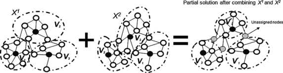
Combination of territories between a pair of solutions


When all trial solutions are generated (i.e., when all pairs of solutions are combined), this set of solutions is improved by using the improvement module previously described. At the end, the improvement process reports a potential set of non-dominated solutions that can be included in the current reference set. Thus, each solution from the potential set enters the reference set if it is a non-dominated solution with respect to the current set of solutions belonging to the reference set. Those solutions that are dominated by the new solution are removed from the current reference set. The SSMTDP stops when there are no new solutions included in the reference set.
Algorithm 1 shows a pseudocode of the proposed SSMTDP. The SSMTDP stops either by iteration limit or by convergence, that is, when the reference set does not change in two consecutive iterations. Note that the updating of the reference set takes place after a potential set of non-dominated solutions is obtained by applying the improvement module over all trial solutions (\(X^{z_{1}}\), \(X^{z_{2}}\), and \(X^{z_{3}}\)) generated by the combination module. This strategy was adopted due to the fact that the computational effort increases considerably when the typical strategy (i.e., updating after each new feasible solution is generated) is performed.

General scheme of SSMTDP
4 Experimental work
The procedure was coded in C++, and compiled with the Sun C++ compiler workshop 8.0 under the Solaris 9 operating system and run on a SunFire V440. The data sets were taken from the library developed by Ríos-Mercado and Fernández (2009). These data set contains randomly generated instances based on real-world data provided by a firm. The SSMTDP was applied over two instance sets with (n,p)∈{(500,20),(1000,50)}. For each set, 10 instances were generated and a tolerance parameter τ (2)=0.05 was used for all of them. Two stopping criteria were used in the SSMTDP, iteration limit and convergence. In these experiments, the maximum number of iterations was set to 10.
4.1 Assessing the performance of SSMTDP
During the experimental work, it was observed that SSMTDP converged without reaching the iteration limit over all instances tested. Thus, in all cases the SSMTDP stopped when there were no new solutions to be added to the reference set. Figure 3 shows the performance of SSMTDP for the instance DU500-08, having 500 BUs and 20 territories. The first frontier (BGRASP-I) is the initial solution set generated by the diversification module (BGRASP-I). The following frontiers show the solutions belonging to the reference set on each SSMTDP iteration. Recall that SSMTDP starts with a non-dominated solution set that is obtained by the diversification module. These solutions are assigned to the initial reference set. After that, each pair of solutions in the reference set is combined to generate three different solutions. The new generated solutions are improved through the RLS and then, the updating of the reference set is done for obtaining a new reference set. When the reference set does not change anymore, the SSMTDP stops. In the case illustrated in Fig. 3, the SSMTDP converged at iteration 9. That is, in this iteration, the combination of solutions from the reference set did not yield potential non-dominated solutions to be added to the reference set. Thus, SSMTDP reports as non-dominated solutions set those solutions belonging to the reference set in the last iteration.

Performance of SSMTDP, instance DU500-08
To illustrate the behavior of SSMTDP by using instances of size (1000,50), Fig. 4 shows the SSMTDP iterations over the instance called DU1000-04 which has 1000 BUs and 50 territories. In this case the SSMTDP stopped in iteration 8. In summary, the approximate efficient frontiers obtained by SSMTDP represent a significant improvement with respect to the initial frontiers provided by BGRASP-I. It was observed that in all instances tested (20 instances), the SSMTDP method stopped by convergence.

Performance of SSMTDP, instance DU1000-04
In the following sections, SSMTDP is compared with two other state-of-the-art heuristics, NSGA-II and SSPMO. NSGA-II is selected as it is the most widely used and cited genetic algorithm for Multiobjective Optimization and, thus, considered a standard for experimental comparisons. On the other hand, SSPMO is regarded as one the most successful and cited non-genetic algorithms for multiobjective optimization. SSPMO is a SS based method that uses the Relinked Local Search principle, whose efficiency has been consistently reported in the literature. Thus, we consider these two methods as important and relevant for benchmarking our proposed heuristic.
Different performance measures have been used for evaluating the quality of the solutions obtained from different multiobjective approaches. Here we consider the most popular measures which have been reported in the literature of multiobjective optimization:
-
1.
Number of points in the non-dominated frontier: It is an important measure because non-dominated frontiers that provide more alternatives to the decision maker are preferred to those frontiers with few non-dominated points.
-
2.
k-distance: This density-estimation technique used by Zitzler et al. (2001) in connection with the computational testing of SPEA2 is based on the kth nearest neighbor method of Silverman (1986). This metric is simply the Euclidean distance from a non-dominated point to the kth nearest non-dominated point. Since the k-distance is defined for a single point in the frontier, two measures are considered in the evaluation of the results, namely, the average and maximum k-distance values computed over all the points of the non-dominated frontier obtained by the method. Thus, the smaller the k-distance for the points in the frontier, the better the frontier density. We use k=4.
-
3.
Size of space covered (SSC(X)): This metric was suggested by Zitzler and Thiele (1999). For a given set of points X, SSC(X) is the volume of the points dominated by X. Hence, the larger the value of SSC(X), the better X. Specifically, let X={X 1,…,X k} be a set of k decision vectors. The function SSC(X) gives the volume enclosed by the union of the polytopes P 1,…,P k , where each P i is formed by the intersections of the following hyperplanes arising out of X i, along with the axes: for each axis in the objective space, there exists a hyperplane perpendicular to the axis and passing through the point (f 1(X 1),…,f k (X k)). In the two-dimensional case, each P i represents a rectangle defined by the points (0,0) and (f 1(X i),f 2(X i)). To avoid computing infinite volumes, the computed volume is divided by the volume of a reference hypercube (setting both upper and lower bound limits for each objective) thus the final result is shown in percentage.
-
4.
C(A,B): It is known as the coverage of two sets measure (Zitzler and Thiele 1999). This measure represents the proportion of points in the estimated efficient frontier B that are dominated by the non-dominated points in the estimated frontier A. Thus, C(A,B) is the coverage of B by points in A.
4.2 Comparison with existing multiobjective SS procedure
4.2.1 Dealing with territory connectivity
Before describing the existing methods used for benchmarking, we must point out an important aspect that is a key difference among these methods. As it has been empirically shown the search space becomes very restricted when the connectivity constraints are considered as hard constraints. Thus, to deal with this issue, a strategy where these constraints are treated as soft constraints is followed in the adaptation of the existing algorithms. That is, these constraints are relaxed and added to a merit search function as a penalty term. By proceeding this way, the algorithms can make a better search in the solution space. Naturally, infeasible solutions are discarded at the end. This strategy contrasts with the one used in the proposed scheme, where this connectivity is explicitly dealt with.
Description of SSPMO
SSPMO is a metaheuristic introduced by Molina et al. (2007) initially developed for solving non-linear multiobjective optimization problems; however, it has been adapted for multiobjective combinatorial problems as well. It consists of a scatter/tabu search hybrid procedure that includes two different phases: (i) generation of an initial set of non-dominated points through Relinked Local (Tabu) Searches (MOAMP), and (ii) combination of solutions and updating of the non-dominated set via scatter search.
The generation of the initial set is based on the MOAMP method proposed by Caballero et al. (2004). To build the initial set of non-dominated points, MOAMP carries out a series of Relinked Tabu Searches where each visited point could be included in the final non-dominated set. The second phase of MOAMP consists of an intensification search around the initial set of non-dominated points. For more details see Caballero et al. (2004), Molina et al. (2007).
The SSPMO procedure creates a reference set (E) using the non-dominated solutions reported by MOAMP. A list of solutions that have been selected as reference points is kept to prevent the selection of those solutions in future iterations. Then, each solution that is added to the set E, is added to a Tabu Set TS. A linear-combination method is used to combine reference solutions. All pair of solutions in E are combined and each combination yields four new trial solutions. Each new solution is subject to an improvement method based on MOAMP. Solutions generated after the improvement procedure are tested for possible inclusion in E. Once all pairs of solutions in E are combined and the new trial solutions are improved, SSPMO updates the reference set E and proceeds to the next iteration. For a complete description of SSPMO method, see Molina et al. (2007).
The SSPMO method was adapted to the multiobjective commercial territory design problem. Four objective functions are minimized: (i) dispersion (6), (ii) maximum deviation with respect to the average number of customers (7), (iii) total infeasibility with respect to the balancing constraints of sales volume (8), and (iv) total number of disconnected nodes. A node is said to be disconnected from a given territory if there is no path between this node and the corresponding territory center considering only edges in this territory. The initial solution set fed to MOAMP is generated by choosing p seeds (configuration of centers) and each of the remaining BUs is assigned to its closest center. The maximum number of updates of the reference set was set to 10 (equal to the number of iterations used in SSMTDP), the maximum number of tabu solutions was set to 55, the threshold value was set to 0.05, and the maximum number of non-dominated solutions included in the reference set was set to 100. The neighborhoods are the same as those defined in the NSGA-II method (following section). For each pair of solutions, four new trial solutions are generated.
At the end, the non-dominated solutions reported by SSPMO are filtered using only those feasible solutions that are non-dominated with respect to the dispersion measure and the maximum deviation with respect to the average number of customers.
Comparing SSPMO and SSMTDP
In this part of the computational work, the SSMTDP procedure is compared with SSPMO. Both SS-based procedures stop by convergence or by iteration limit (10 updates of the reference set). Figure 5 shows the Pareto frontiers provided by SSPMO and SSMTDP. These results correspond to the 10 instances with 500 BUs and 20 territories. The maximum number of allowed movements in SSMTDP was set to 800. Graphically, SSMTDP outperforms SSPMO over all instances tested.


Approximate Pareto frontiers obtained by SSPMO and SSMTDP for the 10 instances tested in set (500,20)
Tables 1 and 2 show a summary of all metrics previously described for evaluating the performance of the algorithms. Clearly, SSMTDP outperforms SSPMO in all metrics for all the instances, specially when considering convergence, where the SSC metric is around twice the one obtained by SSPMO. Additionally, in Table 2 the superiority of SSMTDP over SSPMO is particular evident for instance DU500-04 for which, on average, 90% of the frontiers generated by SSPMO are covered by the frontiers obtained by SSMTDP, and the SSPMO frontiers are not able to cover any point in the frontiers provided by SSMTDP.
In addition, 10 instances with 1000 BUs and 50 territories were tested by applying both SSPMO and SSMTDP using the same stopping criteria as in the previous cases. SSPMO spent more than 30 days without getting convergence for the first instance tested. Then, the stopping criteria was changed and the iteration limit was set to 2. Due that the tremendous computational effort required by the SSPMO, the procedure was not applied to all instances with 1000 BUs and 50 territories. Therefore, here we show only the approximate frontier reported by SSPMO for the instance DU1000-05 (Fig. 6) at iteration 2. In contrast, our procedure SSMTDP converged and reported non-dominated solutions for DU1000-05 and for the remaining instances tested. The maximum number of moves for these cases was set to 2000.

Approximate Pareto frontiers reported by SSPMO and SSMTDP, instance DU1000-05
4.3 Comparison with existing evolutionary algorithm
4.3.1 Description of NSGA-II
The Non-dominated Sorting Genetic Algorithm (NSGA-II) is an evolutionary algorithm that has been successfully applied to many multiobjective combinatorial optimization problems in the literature (Deb et al. 2000) and is the most cited method in multiobjective metaheuristic. Its general description can be found in Deb et al. (2002).
In this work, NSGA-II was adapted to the problem. The same four objective functions already considered for SSPMO are: (i) dispersion (6), (ii) maximum deviation with respect to the average number of customers (7), (iii) total infeasibility with respect to the balancing constraints of sales volume (8), and (iv) total number of unconnected nodes. The main features of this NSGA-II procedure are the following. The generation of solutions consists of randomly selecting p seeds from the set of nodes (V) and assigning the remaining n−p nodes to the closest center. NSGA-II uses different non-domination levels (ranks). In a few words, for each solution h two entities are calculated: (i) domination count d h which corresponds to the number of solutions that dominate the solution h, and (ii) a set of solutions D h that are dominated by h. All solutions in the first non-dominated frontier have their domination count equal to zero. Then, for each solution h with d h =0, each member (g) from S p is visited, and its domination count is reduced by one. In doing so, if for any member g the domination count becomes zero, it is put in a separate list \(\bar{Q}\). These members belong to the second frontier. Now, the above procedure is continued with each member of \(\bar{Q}\) and the third frontier is identified. The process continues until frontiers of all levels are identified.
For each pair of solutions two new solutions are obtained. Each new solution copies each center from the one of the parent solutions with the same probability and the assignment process is equal to that of the initial generation. For each generated solution, a random integer number is generated in the range [0,4]. If the random number is equal to 0, then the mutation process is not applied. Otherwise, the mutation process takes place by using the kind of move determined by the generated number. The different neighborhoods used in NSGA-II are defined by the following moves:
-
1.
Select a center and change it for another randomly selected node. Do a re-assignment of nodes using the new configuration of centers.
-
2.
Select a node in the border of a territory and assign this node to the adjacent territory (keeping connectivity).
-
3.
Select a territory r and assign a randomly selected node from an adjacent territory to r.
-
4.
Interchange two nodes between a pair of territories by holding connectivity.
When the convergence criterion is reached, the best non-dominated solutions are filtered to obtain those feasible solutions that are non-dominated with respect to the dispersion measure and the maximum deviation with respect to the average number of customers.
4.3.2 Comparing NSGA-II, SSPMO, and SSMTDP
NSGA-II was applied to the two data sets previously described. The number of generations and the population size were both set to 500. On each generation 250 solutions were combined. NSGA-II reported non-dominated solutions only for the instance DU500-04 (Tables 3 and 4) which has 500 BUs and 20 territories. For the other 19 instances tested NSGA-II did not provide feasible solutions, while SSTDP procedure reported non-dominated solutions for all the tested instances. It was observed how NSGA-II failed on appropriately handling the connectivity constraints. Most of the solutions generated by NSGA-II are highly infeasible with respect to the connectivity constraints, even though the NSGA-II considers this requirement as objective to be minimized. The selection mechanism and the combination modules are not enough to handle these difficult constraints. In contrast, the proposed SSMTDP procedure is specifically designed to take the connectivity into account over all its components. Thus, for this problem, exploiting problem structure definitely pays off. Figure 7 shows the comparison among the SSMTDP, SSPMO, and NSGA-II procedures.

Approximate Pareto frontiers reported by NSGA-II, SSPMO, and SSMTDP, instance DU500-04
Note that a few non-dominated solutions from SSPMO are dominated by the non-dominated set reported by NSGA-II. In addition, both SSPMO and SSMTDP reported non-dominated points in a region that is not covered by the Pareto frontier obtained by NSGA-II.
Table 3 shows again the superiority of SSMTDP that clearly outperforms both NSGA-II and SSPMO, demonstrating the efficiency of the proposed method. We analyzed the single case (instance DU500-04) in which NSGA-II reported feasible solutions. Note that in the k-distance (mean and max), the corresponding values for NSGA-II could not be computed given that we used k=4. The coverage of two sets measure C(A,B) is shown in Table 4, in this table the set A is associated with the rows and B with the columns. Observe that the points obtained by NSGA-II dominated some points obtained by SSPMO. Table 4 shows that NSGA-II dominates 15% of the points reported by SSPMO. For this metric, SSMTDP dominates the frontiers reported by NSGA-II and SSPMO (see Fig. 7). Moreover, NSGA-II reported feasible solutions just for a single instance out of 20 instances tested, while SSMTDP reported feasible solutions for all instances tested. In summary, SSMTDP outperforms both the NSGA-II and SSPMO procedures.
5 Conclusions and future work
In this paper a novel heuristic procedure based on Scatter Search is proposed. Each component of the proposed method called SSMTDP has been designed taking advantage of the problem structure. Empirical evaluation of the method was performed on two large instance sets, consisting of 500 and 1000 BUs respectively. Solutions generated by SSMTDP were compared with solutions obtained by SSPMO, a State of the Art multiobjective method. SSMTDP reported better solutions than SSPMO in all tested instances. In addition NSGA-II an evolutionary algorithm which is a benchmark for multiobjective problems was adapted to the problem. Empirical work revealed that SSMTDP significantly outperformed NSGA-II on all tested instances. Furthermore, it was observed that NSGA-II struggled to obtain feasible solutions in the first place. This was mainly due to the presence of the connectivity constraints.
As a future work the procedure can be extended to more objectives than those presented here, one immediate extension can be to incorporate the load balancing with respect to sales volume. One more interesting extension is the incorporation of the routing cost of delivering the product; this additional feature can be treated either as an objective or as a constraint.
References
Bong, C. W., & Wang, Y. C. (2004). A multiobjective hybrid metaheuristic approach for GIS-based spatial zone model. Journal of Mathematical Modelling and Algorithms, 3(3), 245–261.
Bowerman, R., Hall, B., & Calamai, P. (1995). A multi-objective optimization approach to urban school bus routing: Formulation and solution method. Transportation Research Part A, 29(2), 107–123.
Caballero, R., Gandibleux, X., & Molina, J. (2004). MOAMP: A generic multiobjective metaheuristic using an adaptive memory. Technical report, University of Valenciennes, Valenciennes, France.
Caballero-Hernández, S. I., Ríos-Mercado, R. Z., López, F., & Schaeffer, E. (2007). Empirical evaluation of a metaheuristic for commercial territory design with joint assignment constraints. In J. E. Fernandez, S. Noriega, A. Mital, S. E. Butt, & T. K. Fredericks (Eds.), Proceedings of the 12th annual international conference on industrial engineering theory, applications, and practice (IJIE), Cancun, Mexico (pp. 422–427). ISBN: 978-0-9654506-3-8.
Deb, K., Agrawal, S., Pratap, A., & Meyarivan, T. (2000). A fast elistist non-dominated sorting genetic algorithm for multi-objective optimization: NSGA-II. In M. Schoenauer, K. Deb, G. Rudolph, X. Yao, E. Lutton, J. J. Merelo, & H. P. Schwefel (Eds.), Parallel problem solving from nature—PPSN VI. Lecture notes in computer science (Vol. 1917, pp. 849–858). Berlin: Springer.
Deb, K., Pratap, A., Agarwal, S., & Meyerivan, T. (2002). A fast elitist multiobjective genetic algorithm: NSGA-II. IEEE Transactions on Evolutionary Computation, 6(2), 182–197.
Duque, J. C., Ramos, R., & Suriñach, J. (2007). Supervised regionalization methods: A survey. International Regional Science Review, 30(3), 195–220.
Glover, F. (1977). Heuristics for integer programming using surrogate constraints. Decision Sciences, 8(1), 156–166.
Grilli Di Cortona, P., Manzi, C., Pennisi, A., Ricca, F., & Simeone, B. (1999). Evaluation and optimization of electoral systems. SIAM monographs on discrete mathematics and applications. Philadelphia: Society for Industrial and Applied Mathematics.
Guo, J., Trinidad, G., & Smith, N. (2000). MOZART: A multi-objective zoning and aggregation tool. In Proceedings of the Philippine Computing Science Congress (PCSC), Manila, Philippines (pp. 197–201).
Kalcsics, J., Nickel, S., & Schröder, M. (2005). Toward a unified territorial design approach: Applications, algorithms, and GIS integration. TOP, 13(1), 1–56.
Laguna, M., & Martí, R. (2003). Scatter search: methodology and implementations in C. Boston: Kluwer.
Martí, R., Laguna, M., & Glover, F. (2006). Principles of scatter search. European Journal of Operational Research, 169(2), 359–372.
Molina, J., Martí, R., & Caballero, R. (2007). SSPMO: A scatter tabu search procedure for non-linear multiobjective optimization. INFORMS Journal on Computing, 19(1), 91–100.
Nygreen, B. (1988). European assembly constituencies for Wales—comparing of methods for solving a political districting problem. Mathematical Programming, 42(1–3), 159–169.
Ricca, F. (2004). A multicriteria districting heuristic for the aggregation of zones and its use in computing origin-destination matrices. Information Systems and Operational Research, 42(1), 61–77.
Ricca, F., & Simeone, B. (2008). Local search algorithms for political districting. European Journal of Operational Research, 189(3), 1409–1426.
Ríos-Mercado, R. Z., & Fernández, E. (2009). A reactive GRASP for a commercial territory design problem with multiple balancing requirements. Computers & Operations Research, 36(3), 755–776.
Salazar-Aguilar, M. A., Ríos-Mercado, R. Z., & Cabrera-Ríos, M. (2011a). New models for commercial territory design. Networks & Spatial Economics, 11(3), 487–507.
Salazar-Aguilar, M. A., Ríos-Mercado, R. Z., & González-Velarde, J. L. (2011b). A bi-objective programming model for designing compact and balanced territories in commercial districting. Transportation Research Part C: Emerging Technologies, 19(5), 885–895.
Salazar-Aguilar, M. A., Ríos-Mercado, R. Z., & González-Velarde, J. L. (2011c). GRASP strategies for a bi-objective commercial territory design problem. Journal of Heuristics, doi:10.1007/s10732-011-9160-8.
Scott, M. N., Cromley, R. G., & Cromley, E. K. (1996). Multi-objective analysis of school district regionalization alternatives in Connecticut. The Professional Geographer, 48(1), 1–14.
Silverman, B. W. (1986). Density estimation for statistics and data analysis. London: Chapman and Hall.
Simeone, B. (1978). Optimal graph partitioning. In Atti delle Giornate di Lavoro AIRO, Urbino, Italy (pp. 57–73).
Singh, C. (1987). Optimality conditions in multiobjective differentiable programming. Journal of Optimization Theory and Applications, 53(1), 115–123.
Tavares-Pereira, F., Figueira, J. R., Roy, B., & Mousseau, V. (2007). Multiple criteria districting problems: The public transportation network pricing system of the Paris region. Annals of Operations Research, 154(1), 69–92.
Zitzler, E., & Thiele, L. (1999). Multiobjective evolutionary algorithms: A comparative case study and the strength Pareto approach. IEEE Transactions on Evolutionary Computation, 3(4), 257–271.
Zitzler, E., Laumanns, M., & Thiele, L. (2001). SPEA2: Improving the strength Pareto evolutionary algorithm. Technical Report 103, Computer Engineering and Networks Laboratory (TIK), Swiss Federal Institute of Technology (ETH), Zurich, Switzerland.
Acknowledgements
We are very grateful to the reviewers whose comments helped improve the presentation of this work. This work was supported by the Mexican National Council for Science and Technology under grants SEP-CONACYT 48499–Y and SEP-CONACYT 61903, Universidad Autónoma de Nuevo León under its Scientific and Technological Research Support, grant UANL-PAICYT CE012–09, by Tecnológico de Monterrey under research grant CAT128, and by the Spanish Ministerio de Ciencia e Innovación under project TIN2009-07869. The first author gently acknowledges a doctoral fellowship from Universidad Autónoma de Nuevo León, grant NL–2006–C09–32652.
Author information
Authors and Affiliations
Corresponding author
Rights and permissions
About this article
Cite this article
Salazar-Aguilar, M.A., Ríos-Mercado, R.Z., González-Velarde, J.L. et al. Multiobjective scatter search for a commercial territory design problem. Ann Oper Res 199, 343–360 (2012). https://doi.org/10.1007/s10479-011-1045-6
Published:
Issue Date:
DOI: https://doi.org/10.1007/s10479-011-1045-6