
Abstract
Coordinating a mobile sensor team (MST) to cover targets is a challenging problem in many multiagent applications. Such applications are inherently dynamic due to changes in the environment, technology failures, and incomplete knowledge of the agents. Agents must adaptively respond by changing their locations to continually optimize the coverage of targets. We propose distributed constraint optimization problems (DCOP)_MST, a new model for representing MST problems that is based on DCOP. In DCOP_MST, agents maintain variables for their physical positions, while each target is represented by a constraint that reflects the quality of coverage of that target. In contrast to conventional, static DCOPs, DCOP_MST not only permits dynamism but exploits it by restricting variable domains to nearby locations; consequently, variable domains and constraints change as the agents move through the environment. DCOP_MST confers three major advantages. It directly represents the multiple forms of dynamism inherent in MSTs. It also provides a compact representation that can be solved efficiently with local search algorithms, with information and communication locality based on physical locality as typically occurs in MST applications. Finally, DCOP_MST facilitates organization of the team into multiple sub-teams that can specialize in different roles and coordinate their activity through dynamic events. We demonstrate how a search-and-detection team responsible for finding new targets and a surveillance sub-team tasked with coverage of known targets can effectively work together to improve performance while using the DCOP_MST framework to coordinate. We propose different algorithms to meet the specific needs of each sub-team and several methods for cooperation between sub-teams. For the search-and-detection team, we develop an algorithm based on the DSA that forces intensive exploration for new targets. For the surveillance sub-team, we adapt several incomplete DCOP algorithms, including MGM, DSA, DBA, and Max-sum, which requires us to develop an efficient method for agents to find the value assignment in their local environment that is optimal in minimizing the maximum unmet coverage requirement over all targets. The disadvantage of dynamic domains based on physical locality is that adaptations of standard local search algorithms tend to become trapped in local optima where targets beyond the immediate range of the agents go uncovered. To address this shortcoming we develop exploration methods to be used with the local search algorithms. Our algorithms are extensively evaluated in a simulation environment. We use a reputation model to determine the individual credibility of agents and consider both additive and submodular joint credibility functions for determining coverage of targets by multiple agents. The performance is measured on two objectives: minimizing the maximum remaining coverage requirement, and minimizing the sum of remaining coverage requirements. Our results show that DSA and MGM with the exploration heuristics outperform the other incomplete algorithms across a wide range of settings. Furthermore, organizing the team into two sub-teams leads to significant gains in performance, and performance continues to improve with greater cooperation between the sub-teams.
1 Introduction
Coordinating mobile sensor teams (MSTs) is at the core of many exciting multiagent systems such as rescue teams searching for survivors after a disaster, unmanned vehicles tracking enemy targets on a battlefield, and mobile sensor platforms providing environmental monitoring. The fundamental problem is to position the agentsFootnote 1 to adequately monitor points of interest generally called “targets” (e.g., disaster survivors, military targets, or pollution spills). Sensors have limited effective ranges and the quality of readings may depend on the agents’ locations and environmental conditions. Furthermore, multiple agents must often cooperate to provide sufficient coverage of individual targets, for example triangulating position using readings from multiple sensors or providing redundancy to provide robustness against sensor failure. Optimally choosing where to position agents to meet the coverage requirements in a static setting is a known NP-hard optimization problem.
Distributed constraint optimization problems (DCOPs) are a general model of multiagent coordination that has been successfully applied to several problems in sensor networks [11, 36, 41, 51]. A DCOP is constituted of agents, variables, and (soft) constraints between sets of variables that reflect the costs of assignments to the variables. Each agent has exclusive control over a subset of the variables and knows information relevant to its variables, such as the values that can be assigned (their domains) and the constraints involving them. The goal is to minimize the aggregated costs of the constraints.
In many ways DCOPs are a natural fit for MSTs, which are inherently decentralized. For each agent there is a variable for its location and for each target there is a constraint with costs equal to the unmet coverage requirements of the target for each joint positioning of the agents. Each agent has exclusive control of its own location and has limited computational and communication resources due to cost, size, and power restrictions. These limitations necessitate that computation be distributed over the entire team in order to use all available computational resources (which scales with the number of agents) and avoid a single point of failure. It also allows agents to make use of local knowledge to avoid communication bottlenecks or unacceptably long delays, which is important because agents can typically only communicate directly with other nearby agents. The constraint-based formulation of costs is general enough to model a wide variety of real-world objective functions.
However, DCOPs fall short in two ways. First, all constraints may involve all agents, because every agent can be positioned anywhere in the environment and thus is eligible for covering any of the targets. This results in an exponential-sized constraint structure, which is difficult to solve. Second, DCOPs are static models [13, 24, 26, 31, 50]. In contrast, the coverage problem confronting the agents in realistic applications is highly dynamic.
There are three types of dynamism in MSTs: changes in the environment external to the agents, including targets arising, moving, and disappearing, or target coverage requirements being modified by an outside authority; changes inherent to the agents, including sensor failures [5, 12] resulting in targets being missed or false information being disseminated [22]; and changes in the agents’ knowledge of the environment, such as the presence of targets and the quality with which they can be sensed from different locations. Because of this last type of dynamism, agents must balance “exploration” (e.g., finding new targets or better sensing locations) with “exploitation” (e.g., deciding where to position themselves based on existing information). This tradeoff is complicated by the fact that considering alternative locations is not just an abstract computational step but involves a physical movement to the new location.
In this paper we propose a new model, DCOP_MST, that extends DCOP for the kinds of dynamic changes encountered by MSTs, which may be arbitrary and unpredictable (e.g., the designation of new targets by a human authority), while simultaneously exploiting structure in the MST problem to improve locality in the constraint network. Instead of choosing from among all possible locations, each agent considers only nearby locations. Constraints thus need not involve all agents at all times but only the agents who are close enough to possibly cover the target. The local environment of an agent is defined by its location, its effective sensing range and the distance it can consider traveling (i.e. its mobility range). Both domains and constraints change as the agents move. We note that such a dependency between the selection of a value assignment by the agent to its variable and the content of its local environment is novel but not necessarily unique to MST applications. Thus, we present a more abstract DCOP model that allows the representation of assignment-dependent local environment (ADeLE) problems, ADeLE_DCOP, which DCOP_MST is a specific instance of.
The quality of agents’ sensing abilities (i.e., their “credibility”) in DCOP_MST is calculated by a reputation model, a widely used technique in multiagent systems and sensor networksFootnote 2 [10, 35, 49]. Each constraint is efficiently represented as the remaining level of coverage given the joint credibility of agents within sensing range. The environmental requirements specify the desired level of coverage for targets. Both the environmental requirements and the agent credibilities are updated dynamically and distributedly.
Agents in DCOP_MST compute new positions using distributed constraint optimization. Due to the dynamic nature of the problem and the large number of possible assignments (even in the reduced DCOP_MST model), complete algorithms are not practical and we focus on incomplete local search algorithms instead.
While agents in traditional DCOPs all execute the same algorithm, in this paper we demonstrate that the tension between exploration and exploitation in DCOP_MST is better resolved by using two different algorithms. We partition the agents into two sub-teams, the surveillance sub-team and the search-and-detection sub-team, and develop different algorithms for each. The primary responsibility of the surveillance agents is to maintain coverage over the known targets, with only minor exploration to find new targets or better sensing locations; in a homogeneous team, all agents would be surveillance agents. The search-and-detection agents are chiefly responsible for finding new targets and in an application would likely be equipped with advanced mobility and accurate sensing equipment.
For the surveillance agents we develop two distributed, self-adjusting algorithms based on the Maximum Gain Messages (MGM) algorithm [24, 30] and the Distributed Stochastic Algorithm (DSA) [50], two well-known DCOP algorithms with typically fast convergence, an essential property in a dynamic environment. Both algorithms require agents to be able to efficiently find the best alternative assignment (position), which in DCOP_MST is not trivial. We propose a method that guarantees local optimality, in terms of the maximum remaining coverage requirement, in polynomial time.
The drawback of these algorithms is that they tend to converge to local minima. We show that existing techniques to escape local minima are unsuited for DCOP_MST as they are unable to maintain high-level surveillance in the presence of dynamic events. We thus develop alternative exploration methods that allow the mobile agents to explore the area while maintaining a high level of coverage of the targets that were previously detected. Empirical evaluation with both additive and non-additive (submodular) functions for calculating joint coverage demonstrates the superiority of our algorithms over standard state-of-the-art DCOP algorithms.
The search-and-detection team requires a higher level of exploration, but only limited coordination because agents are individually capable of detecting new targets and no convergence as agents should continually search for new targets. Thus, we design an innovative algorithm based on DSA in which the agents use a function that initially includes only probabilistic knowledge of the location of the targets. The agents update this function by reducing the importance of areas that they recently visited to reflect the reduced probability of finding new targets there. Agents select their next positions according to this function. Our experiments show that in contrast to standard DSA, our algorithm does not suffer from thrashing as the probability for changing locations increases.
Although the sub-goals of the two sub-teams are different and require different algorithms, awareness of the global goal and the subtask of the other sub-team can enable agents to contribute to the effort of agents in the other sub-team [15, 16, 38]. We propose several levels of cooperation and evaluate their impact on the two sub-teams individually and the team as a whole. Agents can easily make use of information they receive from agents of the other team because the DCOP_MST algorithms are already robust to dynamic changes. Our empirical evaluation reveals that a higher level of cooperation improves the performance of both sub-teams and the overall performance of the global team.
The remainder of this paper is organized as follows. Section 2 formalizes the MST coverage problem and presents the DCOP representation and our innovative DCOP_MST model. Section 3 presents local search algorithms for DCOPs and describes in detail the local search algorithms proposed for solving DCOP_MST, for both the surveillance and the search-and-detection sub-teams. Section 4 proposes levels of cooperation between agents from the two sub-teams. Section 5 includes an evaluation of the proposed algorithms performed by the two sub-teams, the complete team performing together, and the effect of the increased levels of cooperation on performance. Related work is presented in Sect. 6. Our conclusions are presented in Sect. 7.
2 Problem statement
In this section we formalize the problem confronting mobile sensor teams, then describe the conventional DCOP representation followed by the description of the novel ADeLE DCOP model. Finally we present our DCOP_MST formulation as a specific instance of ADeLE_DCOP. A simple example problem that will serve to illustrate the different aspects of the model is depicted in Fig. 1 and explained in Sect. 2.1. Definitions of commonly-used notation defined in this section are summarized in Table 1.

DCOP_MST example with three agents. Faint outer rings around each agent depict the mobility range. Dark inner rings show the sensing range with the numeric agent credibilities. Ovals represent the targets with their coverage requirement. “X”s depict possible locations where the agents can position themselves
2.1 Mobile sensor teams
The agents \(\mathcal {A} = \{ A_1, A_2, \dots , A_n \}\) in a mobile sensor team are physically situated in the environment, modeled as a metric space with distance function \(d\). The current position of agent \(A_i\) is denoted by \( cur\_pos _i\); we assume that this position is accurately known by the agent.Footnote 3 We assume that the locations (or positions) that can be occupied by agents are a finite set of discrete points that form a subset of the total environment. These points can either be a discretization of the underlying space or locations that dominate other nearby points in terms of the sensing quality they afford agents located there. In Fig. 1 the environment is the Euclidean plane, agents are depicted by small robots, and possible locations are shown by “X”s.
We assume that time is discretized so that agents compute movements between possible positions. The maximum distance that \(A_i\) can travel in a single time step is its mobility range \( MR _i\). The mobility range of each agent is shown in Fig. 1 by the fainter, outer circle centered on the agent. All “X”s within the circle are locations that the agent can move to in a single time step from its current position.
Agents are only able to effectively sense targets within a limited sensing range. Agents may be equipped with different kinds of sensors, resulting in heterogeneous sensing ranges; the sensing range of agent \(A_i\) is denoted by \( SR _i\). Because of the sensing range constraint, each agent \(A_i\) can observe all targets within a distance \( SR _i\) from \( cur\_pos _i\), and cannot observe any target that is farther away. The sensing ranges are depicted in Fig. 1 by the darker, inner circle centered at each agent.
Agents may also differ in the quality of their sensing abilities, a property termed their credibility. The credibility of agent \(A_i\) is denoted by the positive real number \( Cred _i\), with higher values indicating better sensing ability. We assume that \( Cred _i\) is exogenously provided (for instance, calculated by a reputation model) and accurately represents the agent’s sensing ability; dealing with inaccurate scores is of interest but beyond the scope of this work. When using reputation models in multiagent systems, e.g., SPORAS [49], agents grade each other according to previous actions and use these grades to tune their expectations of each other. In our model, for example, an agent that carries expensive, accurate sensing equipment will start with a high credibility grade. However, if it would transmit conflicting reports, its credibility grade will drop. An agent’s credibility changes over time due to sensor failures, environmental conditions, and movement of the agent. A major consequence of this is that an agent cannot know its credibility at a location without moving to that location. In Fig. 1, the credibility of each agent is shown as a white number in a blue square on the agent’s sensing range circle.
The individual credibilities of agents sensing the same target are combined using a joint credibility function \(F : 2^A \rightarrow \mathbb {R}\), where \(2^A\) denotes the power set of \(A\). We require that \(F\) be monotonic so that additional sensing agents can only improve the joint credibility. Formally, for two sets \(S, S' \subseteq A\) with \(S \subseteq S'\), we require that \(F(S) \le F(S')\).
The targets are represented implicitly by the environmental requirement function \( ER \) which maps each point in the environment to a non-negative real number representing the degree of coverage (as we define shortly) required for that point to be adequately sensed. In this representation, targets are the points \(p\) with \( ER (p) > 0\). Because targets may arise, move, and disappear, \( ER \) changes dynamically. Moreover, \( ER \) can change as the agent team becomes aware of new targets. A major aspect of the mobile sensing team problem is to explore the environment sufficiently to be aware of the presence of targets. In the example presented in Fig. 1 there are five targets shown as red/dark ovals and their numbers represent their \( ER \) values.
Agents within sensing range of a target \(p\) are said to cover the target. Given a target \(p\), the set of agents within sensing range of \(p\) is
The remaining coverage requirement of target \(p\) is the environmental requirement of \(p\) diminished by the joint credibility of the covering agents, down to a minimum value of 0:
where \(\ominus : \mathbb {R} \times \mathbb {R} \rightarrow \mathbb {R}\) is a binary operator (written in infix notation) that decreases the environmental requirement by the joint credibility. For \(x, y, z \in \mathbb {R}\) with \(y > z\), we require that \(x \ominus y < x \ominus z\), so that decreasing the environmental requirement by a higher joint credibility results in a lower remaining coverage requirement.
The global goal of the agents is to position themselves in order to minimize the values of \( Cur\_REQ \) for all targets. In some cases it may be possible to reduce the values of \( Cur\_REQ \) to zero for all targets, reflecting perfect coverage. However in other cases this may not be possible, either because of insufficient numbers or quality of agents, or by definition of \(F\) and \(\ominus \) (we will see an example of this in Sect. 2.1.1). For these cases we consider two specific objectives. The first is to minimize the sum of remaining coverage requirements for all targets, while the second is to minimize the maximum remaining coverage requirement over all targets.
Minimizing either of these objectives is NP-hard [46], as seen by reduction from the set cover problem [29]. In the set cover problem, there is a set of elements (called the universe) and a family of subsets of the universe whose union contains all elements of the universe. A set cover is a subfamily of these subsets whose union contains all elements of the universe. The set cover problem is to find the set cover containing the minimum number of subsets. The idea of the reduction is to create a target for each element and a location for each subset, defining distances so that the location is within sensing range of all elements in its corresponding subset. A set cover of size \(k\) then exists if and only if it is possible to minimize either the sum or maximum of \( Cur\_REQ \) to 0 using \(k\) agents.
2.1.1 Examples
We now consider three specific choices of \(F\) and \(\ominus \) that may arise in different applications. The sum joint credibility function simply sums the individual credibility of agents:
This can be used to model applications of tracking targets with simple sensors such as received signal strength indicators (RSSIs) capable of determining distance but not direction. Triangulating the position of a target requires readings from three different agents, represented by \( ER (p)=3\) for each target \(p\), binary credibilities of 1 for functioning sensors and 0 for non-functioning sensors, and choosing \(\ominus \) to be the standard subtraction operator. The sum joint credibility function can also be used to protect against sensor failure with \( ER (p)\) being the desired level of redundancy for target \(p\). This approach can be extended to sensors that may have different failure rates, as reflected by non-binary credibilities.
A more nuanced approach for robustness models sensor failures probabilistically and seeks to guarantee that each target is covered by a working sensor with some minimum, target-specific probability. In this case, \( Cred _i\) is the probability that the sensor on \(A_i\) will not fail and \( ER (p)\) is the minimum desired probability that target \(p\) is covered by at least one working sensor. This is represented with the complementary probabilistic joint credibility function
to compute the probability that at least one working sensor covers the target and choosing \(\ominus \) to be the subtraction operator.
A related approach can be used for applications that detect sporadic events with sensors that may give false negatives. The goal is to minimize the probabilities that events occur without being detected. In this case \( Cred _i\) is the probability of an accurate reading from \(A_i\) and \( ER (p)\) is the probability that the event occurs at \(p\). This is modeled using \(F_{ cprob}\) to compute the probability that no sensor detects an event, and the probabilistic reduction operator, \(\ominus _{ prob}:\)
so that \( Cur\_REQ (p)\) is the probability that an event occurs at \(p\) without being detected. Note that it is not possible to reduce \( Cur\_REQ (p)\) to 0 for targets with this choice of \(F\) and \(\ominus \).
2.1.2 Sensor Team Organization
As explained earlier, the \( ER \) function represents the targets in the environment. In practice the agents’ knowledge of the targets will be neither static nor complete, due to the limited observational abilities of agents in MSTs and the inherent dynamism in the problem. We assume that if targets appear, disappear, or move, this can only be directly detected by agents within sensing range of the target; if no agent is within range, the change will not be detected. Thus agents must move not only to optimize their coverage of known targets, but also to explore unobserved parts of the environment in order to detect changes in the \( ER \) function. Because the purpose of this exploratory movement is very different from that of coverage-optimizing movement, it is reasonable to expect different algorithms to be better suited for the different purposes.
One way to implement this in an MST is to organize the team into two disjoint sub-teams of agents running different algorithms specialized to each purpose. The surveillance sub-team is primarily responsible for optimizing coverage of targets assuming that their knowledge of the \( ER \) function is accurate. The search-and-detection sub-team is primarily responsible for exploring the environment and communicating detected changes in the \( ER \) function to the rest of the team. The exact mechanism of disseminating these changes to the rest of the team is dependent on the specific communication capabilities of the agents and is beyond the scope of this paper. The simplest approach is to broadcast the change to all agents if possible, or to propagate via flooding if an ad hoc network is used for communication. More sophisticated approaches may restrict changes to specific parts of the team based on geographic location [9] or may utilize the search-and-detection agents as data ferries to physically carry data between parts of the team that are not in communication range [17].
While the two-sub-team approach can be used with homogeneous agents, agent heterogeneity offers the possibility of specialization according to relative strengths of the different agents. In general, determining target importance often requires more sophisticated capabilities than merely covering the target. For example, in a military application, determining importance may require a high-resolution camera to identify the potential target and perform a threat assessment, while covering the target can be performed with a lower resolution camera. Thus we assume that search agents have superior technology and can therefore perform surveillance with relatively high credibility, while surveillance agents cannot determine the importance of a target.
2.2 The DCOP_MST Model
2.2.1 Standard DCOP
Distributed constraint optimization is a general formulation of multiagent coordination problems that has previously been used for static sensor networks and many other applications. A distributed constraint optimization problem (DCOP) is a tuple \(\langle \mathcal{A},\mathcal{X},\mathcal{D},\mathcal{R}\rangle \) where \(\mathcal {A} = \{A_1, A_2, \dots , A_n\}\) is a finite set of agents, \(\mathcal {X} = \{X_1, X_2, \dots , X_m\}\) is a finite set of variables (with \(m \ge n\)), \(\mathcal {D} = \{D_1, D_2, \dots , D_m\}\) is the set of finite domains for the variables, and \(\mathcal {R}\) is a finite set of relations, also called constraints. Each variable \(X_i\) is held (or owned) by an agent who chooses a value to assign it from the finite set of values \(D_i\); each agent may hold multiple variables. Each constraint \(\mathcal {C} \in \mathcal {R}\) is a function \(C : D_{i_1} \times D_{i_2} \times \ldots \times D_{i_k} \rightarrow \mathbb {R}_+ \cup \{0\}\) that maps assignments of a subset of the variables to a non-negative cost. The cost of a full assignment of values to all variables is computed by aggregating the costs of all constraints. Addition is the aggregation operator most commonly considered so that the total cost is the sum of the constraint costs, but other operators, such as the maximum, have also been considered [26, 37]. The goal of a DCOP is to find a full assignment with minimum cost.
Control in DCOPs is distributed, with agents only able to assign values to variables that they hold. Furthermore, agents are assumed to know only of the constraints involving variables that they hold, thereby distributing knowledge of the structure of the DCOP. In order to coordinate, agents must communicate via message passing. It is commonly assumed that agents can only communicate with agents who hold variables constrained with their own variables, called their neighbors [26, 30, 48, 51]. While transmission of messages may be delayed, it is assumed that messages sent from one agent to another are received in the order that they were sent.
2.2.2 DCOP with assignment-dependent local environment (ADeLE_DCOP)
The model we propose for representing problems that include teams of mobile sensing agents is based on the standard DCOP model presented above and includes multiple dynamic elements. Some, e.g., a change in the utility derived when the sensor is located in some position due to the failure of a sensor, were formalized in previous work on dynamic distributed problems as changes in the problem’s data, which are independent of the assignment selection of agents [32, 47]. However, other dynamic elements in our model change due to the value assignment selection of agents. While this property is inherent in applications that include teams of mobile sensing agents, it exists also in other scenarios and applications; for example, when planning a trip the decision to stop in a city can raise multiple concerns and possibilities that were not considered if this stop were avoided.
Thus, we formalize an innovative framework, ADeLE_DCOP, that is based on DCOP and can represent problems in which the content of the local environment of agents depends on their value assignment selection. Then, we will detail DCOP_MST as a specific instance of this framework. In ADeLE_DCOP there is a general domain of values \(g\)-\(dom_i\) for each agent \(i\) that includes all values that it can take. An agent \(i\) also holds a current domain \(cur\_dom_i \subseteq g\)-\(dom_i\) that includes all the value assignments that an agent can assign to its variable with respect to its current value assignment (denoted by \(cur\_ass_i\)).Footnote 4 The content of \(cur\_dom_i\) is determined by a function \(\varPsi (i,v)\) that takes into consideration the current value assignment \(v\) of agent \(i\) to its variable. Furthermore, for each value \(v \in g\)-\(dom_i\) there is a set of values it is constrained with that are included in the \(g\)-\(dom\)s of other agents. Two agents \(i\) and \(j\) in ADeLE_DCOP are considered neighbors if and only if there exists values \(v \in cur\_dom_i\) and \(v' \in cur\_dom_j\) that are constrained.
Thus, the local environment of an agent \(i\) includes two dynamic sets, its current domain (\(cur\_dom_i\)) whose content is dependent on the agent’s current assignment (\(cur\_ass_i\)), and the set of current neighbors (\(cur\_nei_i\)) that depend on the context of \(cur\_dom_i\). Hence, the content of both sets is dynamic and determined by the value assignment selection of the agent.
2.2.3 DCOP_MST
In formulating the MST problem as an ADeLE_DCOP, each agent \(A_i\) holds a single variable for its position with a general domain \(g\)-\(dom\) that includes all possible locations. For each target \(p\) there is a constraint \(C_p\) that relates the agents’ positions to the remaining coverage requirement \( Cur\_REQ (p)\). Because every agent can take a position within sensing range of \(p\) in some combination, \(C_p\) is an \(n\)-ary constraint. The cost of \(C_p\) for each combination of values is equal to \( Cur\_REQ (p)\) given the agents positions.
The inherent dynamism of the MST problem means that the DCOP problem changes over time. The set of constraints \(\mathcal {R}\) changes over time as targets arise and disappear and agents discover new targets. The cost functions represented by the constraints also change over time due to target movement, sensor failures, and changing agent understanding of sensing quality at different locations due to changing environmental factors.
Even as a static problem this is a very challenging DCOP due to the \(n\)-ary constraints, which are known to be problematic for many DCOP algorithms in practice. Furthermore, the standard assumption of communication locality based on constraint participation is rendered meaningless, with every agent able to communicate with every other. This is in stark contrast to actual mobile sensing applications, where communication between agents is usually limited by physical distance.
The DCOP_MST model is a dynamic ADeLE_DCOP formulation that exploits the structure of MST problems without requiring an explicit model of the dynamics. Instead, the agents consider local changes in their position, and react to changes as they occur. As an instance of the ADeLE_DCOP framework presented above, agents hold variables that take value assignments from a dynamic domain. Specifically, each agent \(A_i\) holds a variable for its position that can take a value from a dynamic domain. The function \(\varPsi (i,v)\) includes in \(cur\_dom_i\) all locations within \( MR _i\) of \( cur\_pos _i\); Thus, as the agent moves locations, the content of the current domain changes.
Dynamic domains induce a change in the constraints. Because of the restricted domains, not all variables can take values within sensing range of all targets, and hence the constraints need no longer be \(n\)-ary. Instead, the constraint \(C_p\) for a target \(p\) only involves those agents \(A_i\) whose domains include a location within \( SR _i\) of \(p\). As the domains change, the constraints change as well.
The local environment of agent \(A_i\) is the joint area within \( SR _i\) from all positions within \( MR _i\) from \(cur\_pos_i\), i.e., it includes all targets that the agent can cover after a single move.
A consequence of this is that the set of neighbors for each agent is no longer the full team and it changes over time as the agents move. In DCOP_MST, two agents are considered neighbors if their local environments overlap, i.e., their sensing areas overlap after they both move as much as possible in a single time step toward each other. Denoting the set of neighbors of \(A_i\) by \( cur\_nei _i\), we formalize this by \( cur\_nei _i = \{A_j|d( cur\_pos _i, cur\_pos _j) \le MR _i + MR _j + SR _i + SR _j\}\). Because agents can only communicate with their neighbors, agents in DCOP_MST can only communicate with other agents who are physically nearby, which is more realistic than the conventional DCOP formulation. As with domains and constraints, neighborhoods in DCOP_MST are dynamic.
3 Algorithms for solving DCOP_MSTs
After defining a model for representing MST problems, the next step is to propose algorithms for agents in the DCOP_MST model to use in order to select their position.
The choice of local search for solving DCOP_MST problems is supported by the common standard considerations for selecting local over complete search, namely time limitations and the limit on the size of problems that can be practically solved by complete algorithms. In addition, the following special properties of MST problem also encourage the choice of a local search algorithm:
-
1.
Exploring the entire search space, as required for complete search, would mean that agents take each and every possible position. This is not practical for sensors with limited mobility in a large area.
-
2.
Dynamic changes limit the time that agents have to execute a complete algorithm, because changes that occur during the search for the optimal solution render the computed solution obsolete.
-
3.
The algorithm is expected to maintain reasonable coverage while adjusting to the changes in the problem [19, 25]. While complete search is guaranteed to find the optimal solution in finite time, this may take a very long time and there are no guarantees on the degree of coverage while the optimal final configuration is being computed.
The simplicity of the framework of local search algorithms makes it compatible with a dynamic environment. Many local search algorithms (such as MGM and DSA [30, 50]) evaluate only the current state in each iteration, while in complete algorithms, agents consider information that was inferred in previous steps of the algorithm (e.g., nogoods [39]). This information might not be valid after the problem changes.
3.1 Local search algorithms for solving DCOPs
The general design of most state-of-the-art local search algorithms for DCOPs is synchronous. The MGM algorithm is a simpler version of DBA [48, 50]. In every synchronous step, each agent sends its current value assignment to its neighbors and collects their current value assignments. After receiving the assignments of all its neighbors, the agent computes the maximal improvement (reduction in cost) to its local state it can achieve by replacing its assignment and sends this proposed reduction to its neighbors. After collecting the proposed reductions from its neighbors, an agent changes its assignment only if its proposed reduction is greater than the reductions proposed by all of its neighbors (ties are broken by agents’ indices). A sketch of the MGM algorithm is depicted in Fig. 2. After selecting a random value to its variable (line 1), the agent enters the loop where each iteration is a step of the algorithm. After sending its value assignment to its neighbors and collecting their assignments (lines 3, 4), the agent calculates its best cost reduction and sends it to its neighbors (lines 5, 6). After receiving the possible cost reductions of all of its neighbors the agent decides whether to replace its assignment and on a positive decision reassigns its variable (lines 7–10).

Standard MGM
DSA is very simple and requires fewer messages than MGM for each possible change of value. After an initial step in which agents pick a value for their variable (randomly according to [50]), agents perform a sequence of steps until some termination condition is met. In each step, an agent sends its value assignment to its neighbors in the constraint graph and receives the assignments of its neighbors. After collecting the assignments of all its neighbors, an agent decides using a stochastic strategy whether to keep its value assignment or to change it. A sketch of DSA is presented in Fig. 3. The differences from the MGM algorithm are that largest reductions (LR-values) are not exchanged and that the replacement decision (in line 5) is stochastic. More specifically, in DSA, the replacement decision takes into account whether a replacement of assignment will improve the local state of the agent. If so, a change is made with probability defined by parameter \(p\). Zhang et al. [50] showed that the value of \(p\) has a major effect on the quality of solutions found by DSA.

Standard DSA
3.2 Algorithms for the surveillance sub-team
In this section we assume that the \( ER \) function used by the surveillance team is complete and accurate, and we develop algorithms for the agents in the surveillance team. Note that locality (i.e. the partial information held by agents) in DCOP_MST is implied by the positions, mobility ranges, and sensing ranges of the agents. Thus, only by taking the assignment and physically moving to the position can an agent compute and adjust its domains and constraints.
3.2.1 Selecting the optimal position in range
A crucial requirement for distributed local search algorithms such as MGM or DSA is for agents to be able to efficiently evaluate alternative positions and select the optimal one from among them. While this evaluation of values is trivial in standard DCOPs, it is not straightforward in DCOP_MST. Moreover, the selection algorithm should serve the global objective of the entire team, heuristically guiding the local search process toward high-quality local optima. In this section we propose a method that is optimal for the objective of minimizing the maximum remaining coverage requirement, allowing us to effectively adapt local search algorithms to DCOP_MST.Footnote 5
An immediate, trivial algorithm would be for each agent to choose a position from its domain that covers a target with the highest \( Cur\_REQ \). However, there may be multiple positions that enable coverage of such a target and the agent must choose between them. The intuitive heuristic that we apply is that the agent should choose the position that further enables coverage of additional targets with a smaller \( Cur\_REQ \). To this end, we propose a recursive method, select_pos, for an agent to select its position; pseudocode is presented in Fig. 4. There are two inputs: \(pos\_set\) is the set of possible positions to be considered, and \(func\) is a function that specifies a value for each target within sensing range of the positions in \(pos\_set\). The algorithm behaves as follows:
-
1.
In the first call, \(pos\_set\) is the set of all positions within the agent’s mobility range \( MR _\textit{self}\) of its current position, and \(func = Temp\_REQ\), the current coverage requirement function excluding the coverage of the agent performing the calculation (\(A_\textit{self}\)). Formally,
$$\begin{aligned} Temp\_REQ(p) = {\left\{ \begin{array}{ll} \max \{ 0, ER (p) \ominus F_{A_i \in ( SR _{(p)} \setminus A_\textit{self})} Cred_i \} &{} \text {if}\,A_{self} \in SR_{(p)} \\ Cur\_REQ (p) &{} \text {otherwise}. \end{array}\right. } \end{aligned}$$Fig. 4 
Method for selecting the best alternative position
-
2.
A set \(target\_set\) containing all targets with maximum \(func\) value within sensing range of a position is computed (line 3).
-
3.
Two termination conditions are checked:
-
(a)
If there is only one possible position, it is selected (lines 1–2).
-
(b)
If there are no remaining targets (\(target\_set = \emptyset \)), then any possible position can be selected (lines 4–5).
-
(a)
-
4.
If neither of the termination conditions is met, the agent computes a new set of possible positions, \(possible\_pos\). Ideally, these are positions from which the agent can cover all of the targets in \(target\_set\), but it may be that no such location exists. In this case, the agent chooses a subset of targets to cover (lines 6–7). In particular, the agent chooses the largest subset of \(target\_set\) that can be covered from a single position in \(pos\_set\). This can be accomplished be iterating over all pairs of \(pos \in pos\_set\) and \(target \in target\_set\) and checking if \(d(pos, target) \le SR_{ self}\); this takes \(|pos\_set| \cdot |target\_set|\) time. The agent then computes \(possible\_pos\) to be the positions in \(pos\_set\) within sensing range of all targets in the possibly reduced \(target\_set\) (line 8).
-
5.
A new function \(new\_func\) is then computed, equal to \(func\) but excluding targets that are covered from all positions in \(possible\_pos\) (lines 9–10).
-
6.
The final step is a recursive call to select_pos using \(possible\_pos\) and \(new\_func\) (line 11).

Figure 5 presents an example of the local method described above. Figure 5a shows the first call to select_pos, with the circle representing the agent’s sensor range and the framed number its credibility (5). Points marked by “X” are alternative positions in \(pos\_set\). Targets (as identified by \(func\)) are depicted by ovals with a number showing their importance, and the shaded oval (for the target with importance 7) indicates \(target\_set\). In the second invocation of select_pos (Fig. 5b), \(target\_set\) contains the two targets with importance 5 and \(pos\_set\) is limited to those positions that were within sensing range of the importance 7 target in the previous call. In the third call (Fig. 5c), \(pos\_set\) contains only two positions, neither of which is within sensing range of the target with importance 4. As a result, the \(target\_set\) contains the two targets with importance 3. Because neither of these allows coverage of both targets, \(target\_set\) will be further reduced to a single target in line 9, and hence in the following invocation of select_pos, \(pos\_set\) will contain a single location and the first termination condition will hold. Figure 5d shows the final selection of the algorithm, along with the sensing range around that point and the four targets that are covered from there.

Local method example. a Elimination of irrelevant positions and identification of the most important target in range, b Second elimination of irrelevant positions and mutual targets, c Third elimination of irrelevant positions and mutual targets, d Final selection
3.2.2 Theoretical properties and bounds
The first bound that needs to be established is that the local method performed by each agent in each iteration is efficient, otherwise it is not realistic to assume that agents can complete computation of the optimal alternative position in a single iteration of the algorithm.Footnote 6
Lemma 1
Assuming the maximum number of possible positions within distance \( MR \) of an agent is \(m\), the maximum number of calls to method select_pos that this agent will make in a single iteration of the algorithm is \(m+1\).
Proof
When method select_pos is called for the first time, the set of possible positions includes a maximum of \(m\) members. In each further call to the method, the values of points which are covered from all possible positions (the \(intersect\_area\)) are not included in the function (lines 9–10 of Fig. 4). Consequently, the points in the next generated \(target\_set\) cannot be in sensing range from all possible positions. Because only positions that are in sensing range from all the points in \(target\_set\) are included in the next generated set of possible positions (line 8), in every recursive call the set of possible positions is smaller. Thus, the function can be called \(m+1\) times at most. Note that \(pos\_set\) is not allowed to become empty due to the second termination condition (lines 4–5). \(\square \)
Lemma 2
Assuming the maximum number of possible positions in the \( SR \) of an agent from any target point is \(s\), the number of calls to method select_pos this agent will make in a single iteration of the algorithm is \(s+1\).
Proof
In each call of method select_pos a target set is generated. Only positions within sensing range from all the points in the target set are considered when the function is called again. Therefore, after the first call, the set of possible positions generated cannot be larger than the number of positions within \( SR \) from the points in the target set. The rest of the proof is similar to the proof of Lemma 1. \(\square \)
The conclusion from Lemma 1 is that in the worst case, the running time complexity of a single iteration is \(m^2 \cdot | target\_set |\) (where \(m\) is defined as in Lemma 1), since in each recursive call each possible position is checked to see if it affords coverage of the \(target\_set\). Furthermore, the conclusion from Lemma 2 is that the worst case running time complexity of a single iteration is \((m + s^2) \cdot | target\_set |\) (where \(m\) and \(s\) are defined as in Lemmas 1 and 2). Thus, the running time of a single iteration is the minimum of the two.Footnote 7
Next, the (local) optimality of the method for selecting an agent’s position is established (it is optimal if only the actions of a single agent are considered). The locally optimal selection is essential to ensure the maximum gain property in the MGM algorithm, which is needed to guarantee convergence. We call a position optimal if it minimizes the coverage requirements according to the \( Cur\_REQ \) function, i.e., if it minimizes the maximum \( Cur\_REQ \) value among all points within the sensing range of all the positions that are in the mobility range of the agent.
Lemma 3
In each recursive call of the select_pos method, the set of possible positions includes the optimal position.
Proof
In the first call for the select_pos function, all positions within mobility range are considered. Thus, the optimal position is considered as well. Assume that the selection of possible positions in the \(i\)th call to the recursive method select_pos by agent \(A_j\) is the first that does not include the optimal position.
We differentiate two cases:
-
1.
There exists at least one possible position in the possible positions set of the \(i-1\) call that is within the sensing range of all the points in the \(target\_set\) generated in the \(i-1\) iteration.
-
2.
No possible position in the possible positions set of the \(i-1\) call is within the sensing range of all points in the \(target\_set\) generated in the \(i-1\) iteration.
The consequence of the first case is that there exists an optimal position \(pos'\) that was included in the possible positions of the \(i-1\) call and is not selected to be included in the new set of possible positions. This means that \(pos'\) is not within \( SR _{self}\) (the sensing range of \(A_j\)) of all points in the target set (line 6 of Fig. 4). However, the goal is to minimize the \( Cur\_REQ \) function and the \(target\_set\) includes the points with the largest \( Cur\_REQ \) values not within sensing range from all possible positions found in the \(i-1\) iteration. Thus, the fact that there exists a position that enables coverage of all points in \(target\_set\) contradicts the optimality of \(pos'\).
For the second case, any selection of position will give the same largest remaining requirement. Thus, any selection is locally optimal and the choice of selecting the position that covers the largest number of points in the \(target\_set\) is a heuristic, which hopefully would help in most cases to achieve the global goal.\(\square \)
The optimality of the select_pos function is an immediate corollary from Lemma 3. Since the select_pos method returns either a position that was left last in the possible positions set or one position from a set of positions from which the agent does not have any coverage differences, this selection is optimal with respect to the position selection of a single agent.
The intuition for the heuristic we use in the method is that covering the largest number of points with maximum coverage requirement would leave fewer such points to cover by the other agents and will contribute more to the joint effort.
3.2.3 Adapting local search algorithms to DCOP_MST
After designing an efficient method for finding the optimal position within range for each agent, we can complete the adaptation of the MGM and DSA algorithms to DCOP_MST. It is important to mention that as self-adjusting algorithms, the algorithms should run indefinitely, i.e., after the algorithm converges to a solution it remains active in order to be sensitive to changes [8].
Figure 6 presents the code of the MGM_MST algorithm. The main loop of the algorithm remains almost unchanged from standard MGM presented in Fig. 2. The agents send their assignments (current positions) to the agents that are currently their neighbors. We assume that agents can detect the agents whose ranges overlap with its own as defined in Sect. 2 and update its set of current neighbors.Footnote 8
Method BestPossibleLocalReduction calls method select_pos to find the best alternative position. After it is found, the method returns the improvement that would be achieved by changing to the selected alternative position. This improvement (or ”reduction”) is the difference between the highest \( Cur\_REQ \) values, not including the credibility variable of \(A_{self}\) (\(Temp\_REQ\)), which are covered by the agent when it is located in one of the two positions (the current and the new) and uncovered when it is located in the other (lines 13–15). The possible improvement cannot be larger than the agent’s credibility variable, \( Cred _{self}\), since that is the agent’s maximal contribution to the coverage of any point in the area (line 16).

MGM_MST
Figure 7 presents the code of the DSA_MST algorithm. The decision of whether to change position is stochastic and does not require agents to exchange their largest reductions (LR values). The replacement decision used is the same as in standard DSA.

DSA_MST
3.2.4 Runtime example
Figure 8 presents an example of a DCOP_MST solved by the MGM_MST algorithm. The team includes five mobile sensors. The dashed lines circling each of the sensors depicts their sensing range. This example uses the sum joint credibility function, \(F_{ sum}\) and the standard subtraction operator for \(\ominus \). The mobility range for each agent is considered to be twice the sensing range (this range was left out of the figures in order to simplify the presentation). The agents are required to cover a number of target areas, which are depicted by complete circles each containing a number. The number represents the environmental requirement function \( ER \). In the initial state of this example (Fig. 8a), there are three target areas with \( ER = 3\) and one with \( ER = 10\). The initial credibility assigned to each agent is 5 (depicted as a framed digit above each dashed circle). In the initial state presented in Fig. 8a, all targets are covered as required. The example includes two events. Figure 8b presents the state after the first event, which is a conflict in the reports that triggered a decrease in the credibility of sensors 1 and 2. As a result, the difference between the requirements on the target and the sum of the credibilities of agents 1 and 2 is 4. Agent 5 is currently covering a target with \( ER \) value of 3. Thus, it moves to a position where it covers the target that is considered more important. The resulting state is presented in Fig. 8c. Agent 4 can improve its local state by moving to a position from which it covers the target it covered before and the target that agent 5 left uncovered (resulting in the state presented in Fig. 8d). Notice that agent 4 moves although it is already covering a target with \( ER =3\), since even though it is covering the point with the largest \( Cur\_REQ \) value in its range, the recursive function requires it to keep considering the different positions that cover this point and possibly additional points with a similar or smaller \( Cur\_REQ \) value. Figure 8e presents the state after an environmental change (the second event). A new target was added with \( ER = 3\). Agent 1 changes its position since its contribution to the coverage of the target it is currently covering is less than its contribution when covering the new target. The final state is presented in Fig. 8f.

Runtime example. a initial state, b credibility change for some of the sensors, c first step of adjustment, d second step of adjustment, e environmental change, f final adjustment
3.2.5 Exploration methods
Classic local search combines exploitation methods in order to converge to local optima with exploration methods in order to escape them [52]. The proposed MGM_MST algorithm is strictly exploitative. It benefits from quick convergence and avoids costly moves by the sensors. However, once a target is beyond the agent’s range it remains uncovered. DSA_MST has an inherent exploration element. However, the results presented in Sect. 5 will reveal that this element is not enough to escape local optima in MST problems. Algorithms that implement methods that enhance local search were proposed for standard DCOPs [24, 30, 50]. However, some of the methods that are most effective in standard DCOP are not expected to be effective for DCOP_MST.
For standard DCOPs, a K-opt solution that can be found by a K-opt algorithm [30] gives an upper bound on the distance from the optimal solution. This guarantee is achieved by allowing any group of \(K\) agents to consider all the constraints they are involved in. As a result, all of the problem’s constraints are considered by groups of \(K\) agents. In DCOP_MST, if a target is not in the range of any agent it will not be considered. Therefore, a K-opt algorithm is expected to allow agents to converge to a deployment that results in better coverage of the targets in range, but it cannot offer the same guarantees as in standard DCOPs when there are targets outside of the agents’ ranges.
Another method that is most effective for standard DCOPs is the anytime framework proposed in [53]. In this framework, agents store the best solution that was explored and this solution is reported when the algorithm is terminated. In DCOP_MST, agents change their physical position and are expected to maintain coverage of targets that were detected. Changing to the best solution can require agents to travel a long distance and at the same time leave targets uncovered. In addition, the method is effective only for static problems since there are no guarantees on the quality of the solution when the problem changes. Thus, holding the best position found so far in memory while exploring for new targets is not expected to be effective for DCOP_MST.
In order to explore the area for new targets while maintaining coverage of targets that were previously detected we propose three simple but powerful exploration methods. Two are combined with the MGM_MST algorithm and one with DSA_MST. These three methods change the parameters of the algorithm temporarily in order to escape local minima. This approach was found to be successful for local search in DisCSPs [3].
-
1.
MGM with Periodic Double Mobility Range (MGM_PDMR) allows an agent to consider points within a larger (double) range than their \( MR \) for a small number of iterations. This method assumes that a wider range is possible even though the iteration will take longer. Therefore, the agents consider a wider range only in some of the algorithm’s iterations, which repeat periodically (in our experiments, for example, for two iterations out of every five we used \(2 \cdot MR \) instead of \( MR \)).
-
2.
MGM with Periodic Incremented Largest Reduction (MGM_PILR) allows agents in some iterations to move to a position that results in an increase of the \( Cur\_REQ \) function up to a constant bound \(c\). More specifically, line 8 of the algorithm is changed in these iterations to: 8. if (\(LR+c > 0\)) Again, this reduced condition is only temporary and is applied periodically. This would mean that for a small number of iterations the importance (coverage requirement) of targets in the area is reduced. Notice that the \(c\) parameter defines by how much they are reduced and thus, fine tuning it would avoid abandoning targets.
-
3.
DSA_PILR is similar to MGM_PILR, only here the same approach of periodic reduced condition is implemented within the DSA algorithm and not within MGM. More specifically, in the iterations where the condition is reduced, the algorithm performs moves even if the reduction is negative up to \(c\).
In all of the proposed methods, agents are not expected to leave targets with high importance in order to search for new targets. This is obvious in MGM_PDMR since, as in the case of MGM_MST, only moves that result in a gain are performed. In the case of MGM_PILR and DSA_PILR, the \(c\) parameter defines the reduced importance of the targets that are already covered. Thus, in MGM_PILR \(c\) is a bound on the increase to the \( Cur\_REQ \) function that the method can create by a single move.
3.2.6 Adapting incomplete inference algorithms to DCOP_MST
The algorithms discussed until now have been local search algorithms. Another family of approaches for solving DCOPs are inference algorithms, in which agents do not propagate assignments but rather calculate utilities (or costs) for each possible value assignment of their neighboring agents’ variables. One of the most popular incomplete algorithm at present is Max-sum, which has been the subject of intensive recent study [11, 41, 54]. Max-sum operates on a cyclic, bipartite factor graph of variable-nodes and function-nodes which represent the agents’ states and constraints, respectively. The complexity of a single iteration of Max-sum is exponential in the degree of the function-nodes (i.e., the constraint arities).Footnote 9 We note that in Max-sum agents act on behalf of variable-nodes and function-nodes in the factor graph. Commonly, agents act on behalf of variable-nodes representing their own variables. Function-nodes can be allocated to agents arbitrarily, deterministically, e.g. by index (as in [54]) or by representing the allocation problem itself as a DCOP and solving it using local search methods (as suggested in [28]). In any case, the allocation does not affect the actions performed by the algorithm. However, if the allocation is not balanced then the complexity of an iteration can increase (when many function-nodes are allocated to the same agent).
Previous work that investigated applications including mobile sensors that need to follow a path and gather information, modeled such scenarios using the DCOP framework by representing mobile sensors as agents that need to select locations and their tasks/targets as constraints, and suggested to solve them using the Max-sum algorithm [41]. However, if all possible future moves of dynamic agents are considered, then all agents are considered for each task and the constraints’ arity is linear in the number of agents. Thus, the problem becomes unsolvable for Max-sum even though it is an incomplete algorithm. Previous work deals with the inherent dynamism of such scenarios by suggesting an iterative process. In each iteration a DCOP instance is built representing the current situation (e.g., sensor positions) and in which only limited movements of the agents are considered. Agents run a distributed algorithm (that might involve several communication cycles) to decide what would be the best next joint move. After they execute the selected joint move, they build a new DCOP instance considering their new positions [41]. This approach generates inherent locality for agents, i.e., in each iteration an agent only considers alternative positions it can move to (in this iteration) and tasks it can fulfill (targets it can cover) when located at these positions.
Thus, we apply Max-sum to DCOP_MST by adjusting the framework suggested in [41] as follows:
-
1.
Select a random assignment.
-
2.
Generate a factor graph according to the current assignment where each sensor is a variable-node and each target is a function-node. Variable-node \(i\) is connected by an edge to a function-node if and only if the distance between them is less than or equal to the sum of \( MR _i + SR _i\), i.e., the sensor can cover the target after a single move.
-
3.
The agents execute the Max-sum algorithm for a predefined number of iterations.
-
4.
The sensors move to the best position (value assignment) as calculated by the algorithm.
-
5.
A new factor graph is generated according to the new assignment selection and the process repeats itself.
In general this algorithm could consider targets that can be covered after multiple moves by an agent. However, this would result in more sensors in range of each target, thereby increasing the degree of each function-node. This is problematic for Max-sum as it would exponentially increase the running time of each Max-sum iteration.
The number of iterations that Max-sum performs before each assignment (position) selection must be selected with care. On one hand, we would like to allow the information regarding the coverage capabilities of sensors to propagate to other sensors. On the other hand, selecting a large number of iterations can cause a deterioration in the quality of the solution as a result of cycles as reported in [11, 54]. Furthermore, these iterations of Max-sum constitute only a single iteration in the global, multi-iteration deployment algorithm, thus, we do not want to generate unnecessary delays. In our experiments we found that Max-sum converges very quickly and thus, a small number of iterations (5) was sufficient to get best performance.
As mentioned above, the complexity bottleneck of Max-sum is the generation of messages by the function-nodes (targets in the case of DCOP_MST). This complexity is known to be exponential in the number of neighboring agents where, in standard Max-sum, the base in the power formula is the domain size and the exponent is the number of variables involved in the function (the degree of the constraint). A number of papers proposed techniques to reduce the complexity of the calculation required for the generation of messages by the function-nodes in Max-sum [23, 41]. We implemented all of the proposed methods in Max-sum_MST, the version of Max-sum we adjusted to DCOP_MST. It is important to note that while these techniques reduce the effective domain size to two, they do not reduce the exponent of the complexity and thus, the effective number of neighboring sensors that a target can have is limited (and small).
3.3 Algorithm for the search-and-detection sub-team
The first step toward including a search-and-detection team in DCOP_MST is relaxing the assumption that there exists an \( ER \) function that includes the accurate importance of every point in the area. Instead, we assume that the function initially includes some distribution that reflects the probability over the existence of targets in the area. This assumption makes the model compatible with any level of uncertainty from complete entropy (as in [19]) to complete knowledge (as we assume in the section above).
Figure 9 illustrates the initial state of a problem. The example includes two types of agents with different credibility variables. The search-and-detection sub-team is composed of the agents with the higher credibility while the agents with the lower credibility are in the surveillance sub-team. The distribution over the probability to find targets in the area is not uniform. The darker areas are the areas with higher probability. The locations of the targets in this example are as in Fig. 8, but are concealed at this point. The initial \( ER \) function includes this probabilistic information, giving points in areas with higher probability for a target a larger value.

Example of the initial state of the full scenario
The initial \(ER\) function containing the probabilistic information is copied to another (initially identical) function we refer to as the search map (\(SM\)). Search agents use the \(SM\) when they decide on their path in order to detect targets, and they generate and update a new \( ER \) function with the targets they find. The surveillance agents use only the new \( ER \) function, in the same way as described in Sect. 3. Thus, the new \( ER \) function is the device used for communication between the two teams.
The search agents use the \(SM\) function to communicate to each other where they have recently visited and therefore the probability of the existence of a new target is low. This is done as follows:
-
1.
The base value of a point in the \(SM\) function, \(Base_p\), is equal to the value in the initial \(ER\) function. Thus, initially, all points in the \(SM\) function are equal to their base value (notice that these points may have different base values according to the probability for a target to exist at them).
-
2.
A search agent \(sa\) located at some point \(p\) at iteration \(t\), causes a decrease in the value of all points \(p'\) within the sensor range of \(p\). The new value of these points is: \(SM(p',t) = max \{0, Base_{p'} - Cred _{sa}\}\).
-
3.
At each iteration \(t\) in which there is no search agent in sensing range from point \(p\), the \(SM\) value of \(p\) is incremented as follows: \(SM(p,t) = min \{SM(p,t-1) + z, Base_p\}\). The selection of the value of \(z\) determines the intensity in which agents will revisit locations in the area. It should be adjusted to the expected frequency of target appearances.
Figure 10 presents the adjusted DSA algorithm for a Search Agent Team (DSA_SAT) in DCOP_MST. As in the case of the Distributed Simulated Annealing algorithm [2], in DSA_SAT the coordination among agents does not rely on a constant probability alone. In each iteration of the algorithm the \(SM\) value of all points within sensor range of the agent are set to a lower value according to the agent’s credibility (lines 3, 4). In addition, the agent updates the \( ER \) function with the true importance of the points in its sensing range.Footnote 10 Then, the agent selects the best position it can move to by calling function get_best_pos(). The agent moves to this position with probability \(prob\) (lines 7, 8).
Function get_best_pos() selects the point within mobility range for which the sum of the \(SM\) values of points within sensing range from it, is maximal.
4 Cooperation between sub-teams
In the previous sections we described two sub-teams performing in the same area, each with its own task, and a means for communication between them via the \(ER\) function. However, it is reasonable to assume that cooperation between agents from different sub-teams can lead to better results for the following reasons:
-
1.
Although each sub-team has its own task, they are both working towards a common goal.
-
2.
Agents’ efficiency depends on their location. Therefore, it may be the case that an agent from one sub-team is in a position that allows it to serve the task of the other sub-team best.
Common practice in multiagent systems include hierarchical plan structures that allow agents to assist others when working towards a common goal [15, 16, 38]. Specifically to the applications at hand, we assume that search agents have superior technology and can therefore perform surveillance with relatively high credibility, while surveillance agents cannot determine the importance of a target. Thus, we describe the following possible collaborations between the two teams:
-
1.
Search support (\(SS\)): search agents take an active role in the surveillance of targets within their sensing range. In practice, we consider the credibility of the search team agents when calculating the current requirement for coverage of targets within the sensing range of search agents.
-
2.
\(Alert\): agents from the surveillance team increase the value of points in the search map where they suspect there might be a target. Thus, search agents are encouraged to search at these locations. In more detail, a monitoring (surveillance) agent that suspects that there is a target within its sensing range changes the value of this point in the search map \(SM\) to be very large. As a result, search agents are drawn to it.
-
3.
Avoid Abandoning (\(AA\)): search agents do not move to a new location when they are covering targets which are not reasonably covered by surveillance agents, i.e., search agents that locate a target wait for it to be covered by surveillance agents before they continue their search.
All three modes of cooperation described above require agents to be aware of the task of the other team. The \(Alert\) and \(AA\) modes further require that agents communicate with agents in the other team via either the \( ER \) or the \(SM\) functions.
5 Experimental evaluation
The proposed DCOP_MST model was evaluated using a simulator for MST problems. The problems simulated are of an area in which the possible positions are a 100-by-100 grid. Each of the points in the area has an \( ER \) value between 0 and 100. The \( ER \) function initially included 10 random points with maximum requirement of 100. Each problem features 50 agents with their initial positions chosen uniformly at random. The mobility and sensing ranges are given in terms of distance on the grid and are varied in our experiments to demonstrate their effect on the success of the algorithms. We consider the \(F_{ sum}\) joint credibility function with subtraction operator and \(F_{ cprob}\) joint credibility function with \(\ominus _{ prob}\) operator (Sect. 2.1.1).
In experiments using \(F_{ sum}\), the credibility of surveillance agents was initially set to \(30\) and the credibility of search-and-detection agents was initially set to \(50\). These values were chosen so that targets with maximum importance (100) require the cooperation of multiple agents. In addition, this setup allows complete coverage (i.e., \( Cur\_REQ = 0\)) in the optimal case and thus we can evaluate the success of the proposed algorithms relative to the optimum. In experiments using \(F_{ cprob}\), the credibility of surveillance agents was \(0.3\) and the credibility of search agents was \(0.5\). The importance of targets was again set to \(100\) (i.e., events occur with probability 1, expressed as a percentage). Notice, \(F_{ cprob}\) is not additive but rather submodular.
The reputation model used in our experiments was inspired by SPORAS [49]. As in SPORAS, all agents are initiated with similar credibility (or ”reputation value” [49])Footnote 11 and the effect of the events on the credibility of agents is with respect to their current level of credibility. The experiments included three types of events:
-
1.
An environmental event that increases a point in the area to a maximum \( ER \) value. This event can represent an intelligence report that some enemy activity is about to happen at a specific location.
-
2.
The credibility of two neighboring agents decreases by \(25\,\%\) (to \(75\,\%\) of what they had before the event). This event represents a conflict in the reports of the two neighboring agents.
-
3.
The credibility of a single agent decreases by \(50\,\%\). This event represents an agent suffering from some technical problem.
All results presented in this section are averaged over 50 runs of the algorithm solving 50 independently-generated random problems; most graphs include error bounds, except for dense graphs where they were omitted for readability. The random elements in each problem were the location of the targets and the initial location of the agents. Dynamic events were also selected randomly.
5.1 Evaluation of the surveillance sub-team
In the experiments described in this section only the surveillance team was evaluated, i.e., the \( ER \) function that the agents used was accurate and was updated after each dynamic event. Although agents used methods that find a locally optimal assignment in terms of the maximum current coverage, we present two global metrics, the maximum remaining coverage requirement over all targets in the area and the sum of remaining coverage requirements over all targets.
5.1.1 Effects of technology on MGM_MST
The first set of experiments examined the effect that technology (i.e., the sensing and mobility ranges) had on the quality of the basic MGM_MST algorithm. These experiments used problems with 15 dynamic, random events. After each event, we allowed the agents 15 iterations to adjust their positions, then recorded the remaining coverage requirements. The results when joint credibility is calculated using \(F_{ sum}\) are shown in Figs. 11 and 12. Figure 11a shows the maximum remaining coverage requirement for teams of agents with different mobility ranges and a fixed sensing range, while Fig. 11b presents the sum of the remaining coverage requirements for the same teams. Similar results for teams with a fixed mobility range and varying sensing ranges are shown in Fig. 12. Figures 13 and 14 present similar results when the method used for calculating joint coverage is \(F_{ cprob}\).

Effect of varying mobility range on MGM_MST with additive joint credibility function \(F_{ sum}\). a Max remaining coverage requirement, b sum of coverage requirements

Effect of varying sensing range on MGM_MST with additive joint credibility function \(F_{ sum}\). a Max remaining coverage requirement, b sum of coverage requirements

Effect of varying mobility range on MGM_MST with submodular joint credibility function \(F_{ cprob}\). a Max remaining coverage requirement, b sum of remaining coverage requirements

Effect of varying sensing range on MGM_MST with submodular joint credibility function \(F_{ cprob}\). a Max remaining coverage requirement, b sum of remaining coverage requirements
It is clear from these figures that in order for the MGM_MST algorithm to perform well, at least one of the parameters \( MR \) or \( SR \) should be high. Otherwise, the algorithm cannot handle events beyond the agents’ ranges and the difference between the coverage requirements and the actual coverage remains high. In other words, in order to benefit from the quick convergence and monotonicity of the MGM algorithm, the agents must be equipped with technology that enables either a large sensing range or a large mobility range. When the technology is limited, exploration methods are required.
Figures 15 and 16 demonstrate the convergence of the sum of remaining coverage requirements by presenting the result for 25 iterations with no dynamic events.Footnote 12 In Fig. 15 the sensing range is fixed and the mobility range varies; in Fig. 16 the sensing range varies while the mobility range is fixed. The results demonstrate a different pattern in convergence. When the sensing range is static and the mobility range grows, the improvement is approximately steady throughout the run. This is because the fixed mobility range results in a fixed domain size, i.e., a fixed number of alternative positions are considered. Thus, the effect of a larger sensing range from each of them is immediate. On the other hand, when the sensing range is static and mobility range changes, the number of alternative positions available for agents is different; thus, multiple iterations may be required for an agent to detect high quality locations.

Effect of mobility range on convergence of MGM_MST for sum of remaining coverage requirements. a Additive joint credibility function \(F_{ sum}\), b submodular joint credibility function \(F_{ cprob}\)

Effect of sensing range on convergence of MGM_MST for sum of remaining coverage requirements, a additive joint credibility function \(F_{ sum}\), b submodular joint credibility function \(F_{ cprob}\)
Tables 2 and 3 demonstrate that these ranges also have an effect on the communication load. When the ranges are larger, agents may have more neighbors and therefore the number of messages per iteration grows. The results in both tables are similar because the neighboring agents are determined by the sum \( SR + MR \). These results were not dependent on the method used for calculating joint coverage.
5.1.2 Comparison of algorithms and exploration methods
While monotonicity has its benefits, e.g., fast convergence and minor movement by the agents, a monotonic algorithm like MGM_MST is limited (and performs poorly) when targets are beyond the agents’ ranges. In order to overcome this limitation, we implemented the three exploration methods—MGM_PILR, MGM_PDMR, and DSA_PILR—described in Sect. 3.2.5 and compared them to three alternative, explorative DCOP_MST algorithms and four baseline algorithms. In this set of experiments, the ranges for all agents were \( SR = 5\) and \( MR = 10\). The parameter \(c\) in the PILR algorithms was set to \(20\). In all the figures in this set we have the experiments in which \(F_{ sum}\) was used depicted on the left of the figures and the experiments in which \(F_{ cprob}\) was used depicted on the right.
The first alternative DCOP_MST algorithm was DSA_MST, described in Sect. 3. In our experiments the replacement decision was made with probability \(p = 0.6\) when the alternative position had positive reduction (i.e., DSA-A [50]). The second was DBA [50], adapted to DCOP_MST. In DBA_MST, agents that detect that they are in a quasi-local minima (i.e., their \(LR\) is non-positive and so is the \(LR\) of their neighbors) change the \(ER\) function by reducing the value of all the points in their sensing range by one. The third was DSAN_MST, an adaptation DSAN [2], a distributed simulated annealing algorithm for DCOPs. Under this algorithm, each agent chooses a random alternative position within their mobility range in each iteration. If this improves local coverage, the agent moves to the alternative position. If this does not improve local coverage, the agent moves there with a probability that depends on the magnitude of worsened coverage and a temperature which decreases over time. When new events are detected, the temperature is reset.
Speaking generally, DSA_MST is the least explorative of these algorithms, always considering the most locally improving position and only decreasing coverage when neighboring agents both update their positions at the same time. DBA_MST is more explorative, possibly decreasing coverage after becoming trapped in a quasi-local minimum. DSAN_MST is the most explorative, considering random locations and decreasing coverage when neighboring agents simultaneously move or if an agent stochastically decides to take a locally non-improving step.
The first baseline algorithm was a naive, random algorithm (“Random”) in which agents move to a random alternative position within their mobility range in each iteration. The second was a naive, greedy algorithm (“Greedy”) in which agents move to the position within their mobility range that offers the local best coverage in each iteration, given their local knowledge. The other two baselines were greedy algorithms very similar to the approach taken by Krause et al. [20]. In the centralized baseline (“Centralized”), agents were sequentially placed at the positions that minimize the remaining coverage requirement given the collective knowledge of all agents in the team. These positions did not have to be within the mobility range of the agent placed there, and agents were assumed to be instantaneously positioned in the new locations, without needing to travel from their old positions. Thus, the centralized solution is presented as a purely theoretical approximation of the optimal solution at each point in time, without considering whether that configuration of agents could have been achieved. The full knowledge baseline (“Full knowledge”) is similar to Centralized but assumes complete, accurate information of the environmental requirements, including any targets which have not been detected by any agent.
The results in Fig. 17 present the maximum remaining coverage requirement for all eleven algorithms. As in the previous set of experiments, after each of the 15 events, the DCOP algorithms ran for 15 iterations and the results presented are the remaining coverage requirements at the end of these 15 iterations. Unsurprisingly, Random does the worst with at least one target completely uncovered. DBA_MST initially does well but finds progressively worse solutions as its objective function becomes distorted by trying to escape quasi-local minima. DSA_MST, Greedy, and MGM_MST all perform comparably and are generally outperformed by DSAN_MST, although this gap becomes insignificant after 14 random events with the additive joint credibility function.

Comparison of DCOP_MST algorithms for maximum remaining coverage requirement. a Additive joint credibility function \(F_{ sum}\), b submodular joint credibility function \(F_{ cprob}\)
The three proposed exploration methods, MGM_PILR, MGM_PDMR, and DSA_PILR, perform similarly and outperform the other approaches by a large amount. Coverage quality also converges to that of Centralized, supporting the conclusion that the proposed approaches move sensors into effective placements. However, the substantial gap in performance between the Centralized and Full knowledge algorithms indicates that in some problems at least one target that could theoretically be covered is still not covered, even with increased exploration.
Figure 18 presents the sum of remaining coverage requirements for ten of the eleven algorithms; Random performed very poorly and is omitted. These results verify that the proposed exploration methods considerably outperform the classic DCOP algorithms. As before, DBA_MST and DSA_MST did not outperform MGM_MST, while DSAN_MST did. The proposed exploration methods all significantly outperformed DSAN_MST, with DSA_PILR performing the best. The differences between the algorithms are less apparent in the experiments using \(F_{ cprob}\), but the same order is maintained on the quality of the results produced by the algorithms. Furthermore, the relative difference between the Full knowledge performance and DSA_PILR (which converges to the Centralized coverage quality) is much smaller than in Fig. 17, indicating that although DSA_PILR occasionally does not cover every target, it does not leave many targets uncovered.

Comparison of DCOP_MST algorithms for sum of remaining coverage requirements. a Additive joint credibility function \(F_{ sum}\), b submodular joint credibility function \(F_{ cprob}\)
Figure 19 compares the standard local search algorithms, local explorative algorithms, baseline algorithms, and Max-sum. The setup in these experiments is the same as in the experiments presented in Fig. 18 except that the sensing and mobility ranges have been reduced to \( SR =3\) and \( MR =3\). This was necessitated by the running time of Max-sum, which is exponential in the number of agents that can sense a target after a single move. We present only the sum of coverage requirements results because the use of small sensing and mobility ranges resulted in targets being uncovered; thus, all algorithms had similarly large maximum remaining coverage requirements.

Comparison of local search algorithms and Max-sum for sum of remaining coverage requirements. a) Additive joint credibility function \(F_{ sum}\), b submodular joint credibility function \(F_{ cprob}\)
The results indicate that Max-sum performs similarly to standard local search algorithms while the explorative algorithms produce sensor deployments of much higher quality. The differences are substantial for both joint credibility functions. It is important to note that while Max-sum produced similar results to standard local search algorithms in these experiments the standard local search algorithms are able to benefit from larger sensing and mobility ranges while Max-sum cannot due to its computational limitations. Surprisingly, MGM_PILR, MGM_PDMR, and DSA_PILR all outperform Centralized after several random events. This is because the small values of \( SR \) and \( MR \) cause many targets to remain undetected with the Centralized algorithm, which is purely exploitive. By performing explicit exploration, MGM_PILR, MGM_PDMR, and DSA_PILR can detect these new targets and thus adjust positions to cover them.
In the next set of experiments, the importance of dynamic domains and dynamic sets of neighbors (constraint network) in the proposed model was evaluated. Figures 20 and 21 compare the MGM_MST algorithm and the two exploration methods, MGM_PILR and DSA_PILR, which were found to be successful in the experiments of the proposed model (presented in Figs. 17 and 18), only using a fixed constraint network and fixed domains.Footnote 13
The results indicate that when fixed domains and a fixed constraint network are used, as in the standard model, the exploration methods are not effective. In fact, MGM and the explorative algorithms produced similar results. It is clear that the dynamic elements in the proposed model enable efficient exploration.

Maximum remaining coverage requirements of intensive exploration methods when domains and neighbors sets are fixed. a Additive joint credibility function \(F_{ sum}\), b submodular joint credibility function \(F_{ cprob}\)

Sum of remaining coverage requirements of intensive exploration methods when domains and neighbor sets are fixed. a Additive joint credibility function \(F_{ sum}\), b submodular joint credibility function \(F_{ cprob}\)
The success of the proposed exploration methods has a cost as well. Table 4 presents the average distance an agent moves in 15 iterations for the different exploration methods, which improve the performance of MGM_MST and for MGM_MST itself. This measure is important since autonomous mobile sensors are expected to have limited battery power. Unsurprisingly, we observe a large difference between the movement in the monotonic algorithms and the PILR algorithms. It is interesting to notice that although MGM_PDMR allows larger mobility ranges in some iterations, the average motion is much smaller than both PILR versions.
We further evaluate the success of the algorithm that offered the best results in terms of coverage (DSA_PILR) with respect to the frequency of dynamic events. Figure 22 Footnote 14 presents the results of an experiment in which events were triggered with different but constant frequency.Footnote 15 When the number of iterations of the algorithm between events is small (5), the algorithm produces a lower quality solution (larger remaining coverage requirements). It is apparent that a larger number of iterations allows the agents to detect the targets and cover them. On the other hand, as more targets are added, there are fewer “free” agents, and thus the advantage of additional iterations becomes minor.

Effect of varying period of DSA_PILR. a Max remaining coverage requirement, b sum of remaining coverage requirements
In order to investigate the success of our proposed algorithm with respect to the optimal solution, we ran experiments on much smaller scenarios for which we were able to solve the problem optimally using brute force search. We considered problems with 4 agents in a \(12\)-by-\(12\) grid world, with with \(2\) initial targets and 5 other targets that were added as dynamic events. The rest of the details of the experiments were similar to the previously-presented experiments. Figure 23 presents the solution quality as a percentage from the optimal solution. For example, if the sum of the remaining coverage requirements of the optimal solution was \(10\) and the sum for the MGM_MST algorithm was 15, we report \(150\,\%\). Obviously, when we add enough targets, even the optimal algorithm cannot produce a high quality solution; thus, the differences became smaller with additional targets.

Performance of DCOP_MST algorithms relative to the optimal deployment for additive joint credibility function \(F_{ sum}\). a Max remaining coverage requirement, b sum of remaining coverage requirements
5.2 Evaluation of the complete team
In the following experiments, the performance of the complete team including the search-and-detection sub-team was evaluated. The problem simulated is similar to the problems in the experiments above, only in most of the experiments presented in this section, 10 of the 50 agents were search agents and 40 were surveillance agents. The \( ER \) function initially had all points equal to \(0\) (no known targets). The credibility of search agents was set to \(50\) and the credibility of surveillance agents was set to \(30\). The sensing ranges of search agents was set to \(8\), and for surveillance agents set to \(5\) as before. The mobility range of search agents was set to \(15\) while the mobility range of surveillance agents was set to \(10\). The surveillance agents executed DSA_PILR, while the DSA_SAT algorithm was executed by the search agents. There were 20 targets with importance \(100\) which were only revealed once a search agent was located within sensing range of them. Surveillance agents could only cover targets that were previously detected by search agents. However, a target that was not yet detected by a search agent raises the suspicion of a surveillance agent.
In order to present the convergence speed of the algorithms using different levels of cooperation, the following graphs include results according to the agents’ locations after each iteration of the algorithm.
In the next set of experiments we evaluated the success of the algorithm we proposed for the search agent team, DSA_SAT, with respect to the value of the \(prob\) parameter, which determines the level of concurrency and exploration. Figure 24a presents the number of targets detected by the search agents as a function of the number of iterations performed since the search started. The different lines represent different \(prob\) values used by the search agents in the DSA_SAT algorithm. It is clear that the algorithm is most successful for high values of \(prob\). In contrast to standard DSA, high level of exploration does not cause thrashing. This is because the search agents are not required to converge to a solution, as in standard DCOP, but rather keep on searching for additional targets. In standard DCOPs, a high probability to change an assignment causes neighboring agents to change assignment concurrently. As a result, the algorithm fails to converge since a change in an assignment does not result in the desired decrease in cost when neighboring agents change assignments as well. Here, the task of all agents is to explore the area and the success of agents decisions is less dependent on the decisions of others. However, for large \(prob\) values (e.g., \(0.7\) and \(0.9\)), there is no notable difference in performance. Figure 24b presents the same phenomenon when Alert cooperation mode is used. This figure demonstrates the benefit of using this mode of communication between the surveillance agents and the search agents for faster detection of targets.

Number of targets found by search agents using different levels of exploration. a Without \(Alert\), b with \(Alert\)
Figure 25 presents the sum of the coverage requirements over all targets in the area.Footnote 16 In this set of experiments, the initial \(ER\) function included all targets. Thus, there was no need to perform search. The results in Fig. 25 demonstrate the effect of the different levels of communication on the performance of the surveillance team. It is clear from the result that when the search agents participate in the surveillance procedure (\(SS\) mode) but are not committed to it, the improvement in performance is minor. However, when the search agents are aware of the level of coverage on targets found and leave targets only if they are reasonably covered (\(AA\) mode), the performance in terms of surveillance substantially improves.

Total remaining coverage requirements for different levels of cooperation (no search)
Figure 26 presents results of a complete experiment, i.e., target locations are not known in advance and the results are in terms of surveillance coverage (both sub-teams need to perform their sub-task). The results presented demonstrate how each additional level of cooperation between the two sub-teams improves the overall performance of the entire global team of sensing agents (plain means no cooperation at all). It is notable that the \(SS\) mode by itself results in a very small improvement. It turns out that the assistance of the search agents to the surveillance process is effective only if they are somewhat committed to this task. The effect of the \(Alert\) mode is more apparent in the first iterations when surveillance agents are waiting for targets to be discovered. The \(AA\) mode triggers the most substantial improvement in coverage. To emphasize the difference in performance, we take a closer look at the last iterations in Fig. 27 and see that towards the end of the run, in the highest level of cooperation, the coverage of the team is improved by a factor larger than two.

Sum of remaining coverage requirements for different levels of cooperation

Sum of remaining coverage requirements for different levels of cooperation (a closer look)
Figure 28 presents the results when there are different proportions between the sizes of the search sub-team and the surveillance sub-team. The experiments presented on the LHS included \(45\) surveillance agents and \(5\) search agents. The experiments presented on the right included 35 surveillance agents and 15 search agents. It is clear that the number of search agents affects the time until targets are detected and therefore a large search team allows faster convergence.

Sum of remaining coverage requirements for different divisions of agents between the sub-teams. a 45 surveillance agents, 5 search agents, b35 surveillance agents, 15 search agents
Table 5 presents the average number of messages per iteration when using the different levels of cooperation. As expected, the search support mode has a small impact on the total communication and the alert mode has some additional impact as well. The avoid abandoning mode has minimal impact since it does not require additional messages.
Figure 29 presents results of the same experiment on a non-uniform search map. In this experiment the search map contained three 10-by-10 areas with higher probability for the existence of a target. The probability for a target to exist in one of the points in the first special area was twice that of the points outside the high probability areas; the probability for a target in the second special area was three times as great as outside the high probability areas. In the third area, the probability of a target in one of the points was four times that in standard points. The results indicate that the targets are found very quickly and there is a smaller difference in coverage between the different modes in the later iterations. Indeed, additional information helps the search agents detect targets faster. Interestingly, it is apparent that the \(alert\) mode is more successful in the early iterations than the \(plain\) and \(SS\) mode. One could have expected that the alert mode will be less effective here since the search map includes more information for the search agents. This can be explained as follows. There is still a chance that targets will appear outside the special areas. These targets can be missed by the search agents (which are drawn to areas with higher probability) unless there is an alert from surveillance agents.

Total remaining coverage requirements for different levels of cooperation when the initial search map (initial \(ER\)) is non-uniform
In the last experiment we investigated the effect of dynamic events on the performance of the full team. The scenario was similar to the previous experiments with dynamic events, however here, the search agents had to find additional appearing targets and add them to the \( ER \) function. The results in Fig. 30 indicate that the higher levels of cooperation were beneficial. The largest difference found was between the search support mode and the avoid abandoning mode. Thus, the awareness of the global team objective allowed search agents to balance between their support of the surveillance agents and their own task of detecting new targets.

Total remaining coverage requirements for different levels of cooperation on problems with dynamic events
6 Related work
DCOP is a general model for distributed problem solving that has generated significant interest from researchers [7, 14, 24, 26, 31, 50]. A number of studies on DCOPs presented complete algorithms [13, 26, 31, 39]. However, since DCOPs are NP-hard, there has been a growing interest in the last few years in local (incomplete) DCOP algorithms [30, 42, 44, 50, 53]. Although local search algorithms do not guarantee that the obtained solution is optimal, they are applicable for large problems and are compatible with real time applications. The study of DCOP algorithms in dynamic environments is emerging recently [21, 25, 32, 33]. Mailler adapted two distributed constraint satisfaction (DisCSP) algorithms to solve dynamic problems [25]. This pioneering work was the first to evaluate algorithms according to their performance through time and not just after convergence. On the other hand, the problems on which the algorithms were compared were three coloring problems that included dynamic constraints but no other dynamic elements. In this paper we address distributed optimization problems that include more realistic dynamic elements. A short paper by Lass et al. [21] called to the DCR community to show interest and propose models and algorithms for dynamic DCOPs. Our work is clearly a reaction to their call. A different approach was taken by Petcu and Faltings [32, 33], which adjust a complete inference algorithm (DPOP) to a dynamic environment by designing it as a continuous self stabilizing algorithm. Furthermore, by adding costs to assignment changes dynamically, the stability of the solutions obtained was increased [33]. Another study that investigates the adaptation of complete algorithms to a dynamic DCOP is [47]. In this study the authors propose the use of bounds that were found when running a branch and bound based asynchronous distributed algorithms (BnB-ADOPT) when using the algorithm again after the problem changes, in case the dynamic events did not affect their consistency. Obviously the approaches presented above of adjustments of complete search algorithms cannot be applied to scenarios with large teams of mobile sensing agents where agents have limited local environments as we address in this paper.
Previous attempts to cope with the dynamic properties of mobile sensors have focused on a specific element of the problem. One example (mentioned above) is the detection of failing agents, which can be solved by avoiding interaction with them [12]. Although in the case of failure of agents, detection is a first and important step towards the generation of a robust network, detection alone may not be enough. First, the indications for a failure might not be conclusive. Second, a change in the environment can cause the position of the agent to no longer be adequate. Thus, it would probably be more effective to relocate the agent than to avoid interactions with it. Third, in the case of an agent’s failure in an area with high importance, it is not enough to avoid interactions with it. The goal of the team is to maintain high level coverage on such delicate areas; thus, other functioning sensing agents should be moved in that direction.
Another example is the deployment of sensors in an area in order to achieve maximal coverage [18, 34]. In these studies agents make use of virtual potential fields in order to maintain an adequate distance from one another and, thus, maximize the area they cover. In our work, a wider range of problems and tasks of mobile sensor teams is considered that include areas of high importance that require overlapping coverage and sensors with different level of credibility, etc. We note that the max-coverage problem (i.e., cover the largest area) is a specific case of the problems to which our proposed model applies.
Placement of sensors in a static network was studied by Krause et al. [20]. Instead of covering discrete targets, the goal was to maximize the mutual information of spatially distributed phenomena (such as temperature in a building) modeled as a Gaussian process. While solving the problem is NP-hard, the authors presented a near-optimal polynomial-time algorithm that exploited the submodularity of the objective function. This is an example of greedy heuristics providing near-optimal solutions for maximizing submodular functions [27]. While not directly applicable to the MST coverage problem, it may explain why the local search algorithms we developed tend to find high quality solutions.
A number of papers considered DCOP for solving static sensor networks. Some examples are [4, 44]. In [19, 43], the performance of DCOP local search algorithms when the reward function is uncertain is investigated. This property is related to mobile sensor nets when agents do not know the reward of taking a position (value assignment) before they actually take it. Jain et al. [19] reported experiments in which DCOP algorithms were used to solve a realistic problem of robots seeking to maximize radio signals were presented. In [43] the trade-off between the choice to explore new territories vs. the choice to exploit the available information to maximize performance was investigated. These studies clearly put the focus on different elements of mobile sensor applications than our study. The assumption made in our study is that two different teams of agents exist, one whose task is detection and the other whose task is coverage. The search-and-detection team faces uncertainty and provides accurate information for the surveillance team. We propose and evaluate means for cooperation among the two teams.
Stranders et. al. [40, 41] investigate scenarios in which mobile sensing agents must follow a path and gather information. Their approach is similar to ours in the use of the DCOP model having sensors represented by agents and sensing tasks by constraints. The solution method they proposed stemmed from the Max-sum algorithm. Max-sum, however, is not compatible for problems in which constraints have high arity (many agents involved). Thus, in [41] an iterative framework was proposed in which only a limited movement for each agent is considered in each iteration, hence the local environment of agents was limited and the complexity bottleneck of constraint arity reduced. We demonstrate in our empirical study that when applying Max-sum to DCOP_MST using this framework the resulting algorithm outperforms other standard incomplete algorithms that are adjusted to DCOP_MST, but is inferior to specially designed explorative local search algorithms. Moreover, in contrast to local search algorithms, which benefit from a large local environment, Max-sum becomes infeasible when the agent’s local environment grows and the constraint arity with it.
The model presented in this paper is constructed on the ability of a reputation model to detect the quality of agents’ reports (i.e., their credibility). Here we follow common practice in multiagent systems in general and in sensor networks specifically [6, 10, 35, 49]. The following description of the role of a reputation model explains our choice: ”Reputation models enable agents to gather information in richer forms from their environment and make rational inferences from the information obtained about their counterparts” [35]. The information in a reputation model is shared via interactions of agents. This information takes the form of a performance rating that is shared by the nodes in the network [35]. In this paper the rating is used to determine the credibility of agents. Although we present in our experiments a simple model based on SPORAS [49], any model that assigns a numeric scalar value to agents can be used.
The problems we address in this paper and the model presented have some similar elements to the Predator/Prey problem that is studied and draws interest in the multiagent systems community [1]. The similarity comes from the need of multiple predator agents to be within range of a prey in order to accomplish their tasks. In addition, a prey agent is dynamic, as targets can be in our model. The difference is in the requirements of a solution that are much more constrained in the Predator/Prey problem. In the model of Abramson et al. [1], the predator agents are required to surround a prey from four different sides. Therefore, the solutions proposed consider role allocation that defines which predator will be placed on which side of the prey. For a single prey, the problem can be solved efficiently (by a tractable algorithm) and therefore the most successful algorithm proposed involved predator agents sharing their information and all agents computing the final allocation. The problem with multiple prey agents is NP-hard.
Cooperation among heterogeneous sensors was found to be effective for static sensor/camera networks [45]. Our investigation of cooperation between teams with different types of mobile sensing agents with different tasks, while applying to a different scenario is another indication that efficiency can be achieved via cooperation.
7 Summary and conclusions
In this paper we proposed a new model for representing dynamic coordination problems confronting teams of mobile sensing agents. Our model, DCOP_MST, extends the well-known distributed constraint optimization problem framework to dynamic settings, and allows the agents to efficiently coordinate their actions while remaining robust to environmental changes, modifications of the team’s sensing goals, and dynamic variability in the quality of agents’ reports as can be caused by technology limitations or hardware failures.
We demonstrated how the flexibility of DCOP_MST in representing and coping with dynamic elements easily facilitates the organization of the agents into a surveillance sub-team and a search-and-detection sub-team. This enables more efficient use of heterogeneous agents (e.g., dedicating agents equipped with advanced mobility technology to finding new targets) and allows the system designer to deploy algorithms that are suited to each sub-team’s goal. We also develop several methods of increasing cooperation between sub-teams, and empirically show how increasing levels of cooperation improves the performance of both sub-teams individually as well as the team as a whole.
For the search-and-detection agents we proposed an algorithm based on DSA that our results demonstrated was most successful with a high level of exploration. For the surveillance team, we developed an efficient method that allows agents to find the (locally) optimal alternative assignment/position. We showed how this method can be used to adapt incomplete DCOP algorithms such as MGM, DSA, DBA, and Max-sum to the DCOP_MST model. Our experimental study found that the local search algorithms (MGM, DSA, and DBA) became trapped in local optima due to insufficient exploration. We thus developed three new exploration methods that enable agents to search for targets that are currently beyond their sensing range while maintaining acceptable coverage on previously detected targets. Our experimental results demonstrated the superiority of using these exploration methods compared to the naive local search algorithms or Max-sum.
While our paper focused on applications that include teams of mobile sensing agents we note that the special type of dynamism inherent in DCOP_MST, i.e., the ADeLE, is also relevant in many other applications. Thus, we presented the more abstract ADeLE_DCOP model for representing such problems, which DCOP_MST is a specific instance of. Our results encourage further investigation of distributed AI applications that fall under this category and can be represented as ADeLE_DCOPs, e.g., robot movement and distributed planning, in which the set of alternative assignments and relevant constraints depend on the current assignment of agents. Prior to our study, DCOP was not considered as an appropriate choice for representing such applications because of its static model. We are convinced that our main contribution is the broader set of applications for which DCOP will be used to represent and solve in the future.
In future work we intend to relax some of the assumptions used in the model, e.g., the accuracy of the reputation model and the ability of search agents to precisely evaluate the importance of targets. Such inaccuracy is expected to require solutions that are more robust.
Notes
In this paper we assume that each agent resides on a mobile sensor and we use the terms agent and sensor interchangeably.
We leave the problem of handling inconsistent information caused by malicious activity for future work.
This is a reasonable assumption considering that GPS receivers are used.
For simplicity of presentation and without loss of generality we assume that each agent holds a single variable
In Sect. 5 we present experimental results showing that our approach is also effective for the objective of minimizing the sum of remaining coverage requirements.
In our proof we assume that there are no plateaus (continuous areas with the same \( ER \) value) and that the number of points of the same (highest) value can be found efficiently. If plateaus do exist, the proof is still valid; however, there is a need to use geometric computation in order to evaluate areas instead of points.
In contrast to the assumptions made, in case the initial possible position set or target set are too large and the method cannot be completed in reasonable time, the method can be stopped and one of the positions in \(pos\_set\) can be selected. However, in this case local optimality is not guaranteed.
If not, agents would need to inform all other agents when they change position so that they can update their set of neighbors accordingly.
importance(\(p\)) in line 5 is the true importance of point \(p\) sensed by the agent.
Fig. 10 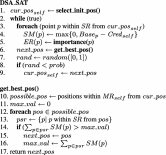
DSA_SAT
In contrast to SPORAS, the initial credibility is not zero since in MSTs we are not concerned with agents using different pseudonyms.
We omit the maximum remaining coverage here because the effect is not notable until all targets are located.
Notice that the MGM_PDMR method reduces to MGM_MST when the domains are fixed and therefore is not evaluated in this experiment.
Beginning with this experiment, we present only the results for the \(F_{ sum}\) method. The results in the experiments using \(F_{ cprob}\) were consistently similar with less apparent differences between the algorithms.
We do not present error bars in this graph because they make the figure unreadable due to the similarity of the results.
In the rest of the figures the error bounds were omitted due to the density of the graphs.

References
Abramson, M., Chao, W., & Mittu, R. (2005). Design and evaluation of distributed role allocation algorithms in open environments. In Proceedings of the 2005 International Conference on Artificial Intelligence 2005, IC-AI 2005 (pp. 565–571).
Arshad, M., & Silaghi, M. C. (2004). Distributed simulated annealing. In Distributed constraint problem solving and reasoning in multi-agent systems, frontiers in artificial intelligence and applications series (Vol. 112), November 2004.
Basharu, M., Arana, I., & Ahriz, H. (2007). Solving coarse-grained DisCSPs with Multi-DisPeL and DisBO-wd. In IAT ’07: Proceedings of the 2007 IEEE/WIC/ACM international conference on intelligent agent technology, Washington, DC, USA (pp. 335–341).
Bejar, R., Domshlak, C., Fernandez, C., Gomes, K., Krishnamachari, B., Selman, B., et al. (2005). Sensor networks and distributed CSP: Communication, computation and complexity. Artificial Intelligence, 161(1–2), 117–148.
Braginsky, D. (2002). Rumor routing algorithm for sensor networks. In Workshop on wireless sensor networks and applications (WSNA), Atlanta, Georgia, USA, September 2002 (pp. 22–31).
Buchegger, S., & LeBoudec, J. Y. (2005). Self-policing mobile ad-hoc networks by reputation. IEEE Communication Magazine, 43, 101–107.
Chechetka, A., & Sycara, K. (2006). No-commitment branch and bound search for distributed constraint optimization. In AAMAS ’06: Proceedings of the fifth international joint conference on autonomous agents and multiagent systems, New York, NY, USA (pp. 1427–1429).
Collin, Z., Dechter, R., & Katz, S. (1999). Self-stabilizing distributed constraint satisfaction. Chicago Journal of Theoretical Computer Science, 5.
Delot, T., Ilarri, S., Cenerario, N., & Hien, T. (2011). Event sharing in vehicular networks using geographic vectors and maps. Mobile Information Systems, 7(1), 21–44.
Du, R., Xu, M., & Zhang, H. (2006). An extended hierarchical trusted model for wireless sensor networks. Wuhan University Journal of Natural Sciences, 11, 1489–1492.
Farinelli, A., Rogers, A., Petcu, A., & Jennings, N. R. (2008). Decentralised coordination of low-power embedded devices using the max-sum algorithm. In 7th International conference on autonomous agents and multi-agent systems, AAMAS-08 (pp. 639–646).
Frye, L., Liang, C., Du, S., & Bigrigg, M. W. (2006). Topology maintenance of wireless sensor networks in node failure-prone environments. In Proceedings of IEEE international conference on networking, sensing and control, April 2006 (pp. 886–891).
Gershman, A., Meisels, A., & Zivan, R. (2006). Asynchronous forward-bounding for distributed constraints optimization. In Proceedings of the 17th European Conference on Artificial Intelligence (ECAI 2006), August 2006 (pp. 103–107).
Gershman, A., Meisels, A., & Zivan, R. (2009). Asynchronous forward bounding. Journal of Artificial Intelligence Research, 34, 25–46.
Grosz, B. J., & Kraus, S. (1996). Collaborative plans for complex group action. Artificial Intelligence, 86(2), 269–357.
Grosz, B. J., & Kraus, S. (1999). The evolution of SharedPlans. In A. Rao & M. Wooldridge (Eds.), Foundations and theories of rational agency (pp. 227–262). Dordrecht: Kluwer Academic Publisher.
He, T., Lee, K.-W., & Swami, A., (2010). Flying in the dark: Controlling autonomous data ferries with partial observations. In Proceedings of the eleventh ACM international symposium on mobile ad hoc networking and computing, MobiHoc ’10 (pp. 141–150). New York, NY: ACM.
Howard, A., Matarić, M. J., & Sukhatme, G. S. (2002). An incremental self-deployment algorithm for mobile sensor networks. Autonomous Robots Special Issue on Intelligent Embedded Systems, 13(2), 113–126.
Jain, M., Taylor, M. E., Yokoo, M., & Tambe, M. (2009). DCOPs meet the real world: Exploring unknown reward matrices with applications to mobile sensor networks. In Proceedings of the twenty-first international joint conference on artificial intelligence (IJCAI-09), Pasadena, CA, USA, July 2009.
Krause, A., Singh, A., & Guestrin, C. (2008). Near-optimal sensor placements in Gaussian processes: Theory, efficient algorithms and empirical studies. Journal of Machine Learning Research, 9, 235–284.
Lass, R. N., Sultanik, E. A., & Regli, W. C. (2008) Dynamic distributed constraint reasoning. In Proceedings of the Twenty-Third AAAI Conference on Artificial Intelligence, Chicago, IL, USA (pp. 1466–1469).
Leskovec, J. (2008). Dynamics of large networks. Ph.D. Thesis, CMU, Pittsburgh, PA, USA.
Macarthur, K. S., Stranders, R., Ramchurn, S. D., & Jennings, N. R. (2011). A distributed anytime algorithm for dynamic task allocation in multi-agent systems. In AAAI.
Maheswaran, R. T., Pearce, J. P., & Tambe, M. (2004). Distributed algorithms for DCOP: A graphical-game-based approach. In Proceedings of parallel and distributed computing systems (PDCS), September 2004 (pp. 432–439).
Mailler, R. (2005). Comparing two approaches to dynamic, distributed constraint satisfaction. In AMAS 2005. Proceedings of the fourth international joint conference on autonomous agents and multiagent systems, Utrecht, Netherlands (pp. 1049–1056).
Modi, P. J., Shen, W., Tambe, M., & Yokoo, M. (2005). ADOPT: Asynchronous distributed constraints optimization with quality guarantees. Artificial Intelligence, 161(1–2), 149–180.
Nemhauser, G. L., Wolsey, L. A., & Fisher, M. L. (1978). An analysis of approximations for maximizing submodular set functions-I. Mathematical Programming, 14(1), 265–294.
Ota, K., Matsui, T., & Matsuo, H. (2009). Layered distributed constraint optimization problem for resource allocation problem in distributed sensor networks. In Principles of practice in multi-agent systems 12th international conference, PRIMA 2009 (pp. 245–260).
Papadimitriou, C. H., & Steiglitz, K. (1982). Combinatorial optimization: Algorithms and complexity. Englewood Cliffs: Prentice-Hall.
Pearce, J. P., & Tambe, M. (2007). Quality guarantees on k-optimal solutions for distributed constraint optimization problems. In International joint conference on artificial intelligence (IJCAI), Hyderabad, India.
Petcu, A., & Faltings, B. (2005). A scalable method for multiagent constraint optimization. In International joint conference on artificial intelligence (IJCAI) (pp. 266–271).
Petcu, A., & Faltings, B. (2005). Superstabilizing, fault-containing multiagent combinatorial optimization. In Proceedings of the national conference on artificial intelligence (AAAI) (pp. 449–454).
Petcu, A., & Faltings, B. (2007). Optimal solution stability in dynamic, distributed constraint optimization. In Proceedings of the international conference on intelligent agent technology (IAT) (pp. 321–327).
Poduri, S., & Sukhatme, G. S. (2004). Constrained coverage for mobile sensor networks. In IEEE International conference on robotics and automation (pp. 165–171).
Ramchurn, S. D., Huynh, D., & Jennings, N. R. (2004). Trust in multi-agent systems. The Knowledge Engineering Review, 19, 2004.
Rogers, A., Farinelli, A., Stranders, R., & Jennings, N. R. (2011). Bounded approximate decentralised coordination via the max-sum algorithm. Artificial Intelligence, 175(2), 730–759.
Schiex, T., Hélène, F., & Verfaillie, G. (1995). Valued constraint satisfaction problems: Hard and easy problems. In International joint conference on artificial intelligence (IJCAI) (Vol. 1, pp. 631–639).
Sen, S., & Durfee, E. H. (1994). The role of commitment in cooperative negotiation. International Journal of Cooperative Information Systems, 3, 67–82.
Silaghi, M. C., & Yokoo, M. (2006). Nogood based asynchronous distributed optimization (ADOPT ng). In AAMAS 2006: Procedings of the fifth international joint conference on autonomous agents and multiagent systems (pp. 1389–1396).
Stranders, R., Delle-Fave, F. M., Rogers, A., & Jennings N. R. (2010). A decentralised coordination algorithm for mobile sensors. In Proceedings of the 24th conference on AI (AAAI).
Stranders, R., Farinelli, A., Rogers, A., & Jennings, N. R. (2009). Decentralised coordination of mobile sensors using the max-sum algorithm. In International joint conference on artificial intelligence (IJCAI) (pp. 299–304).
Sun, X., Yeoh, W., & Koenig, S. (2009). Trading off solution quality for faster computation in DCOP search algorithms. In Proceedings of the international joint conference on artificial intelligence (IJCAI), July 2009 (pp. 354–360).
Taylor, M. E., Jain, M., Jin, Y., Yokoo, M., & Tambe, M. (2010). When should there be a ”me” in ”team”?: Distributed multi-agent optimization under uncertainty. In Proceedings of the 9th conference on autonomous agents and multi agent systems (AAMAS 2010) (pp. 109–116).
Teacy, W. T. L., Farinelli, A., Grabham, N. J., Padhy, P., Rogers, A., Jennings, N. R. (2008). Max-sum decentralised coordination for sensor systems. In AAMAS ’08: Proceedings of the 7th international joint conference on autonomous agents and multiagent systems (pp. 1697–1698). Estoril: International Foundation for Autonomous Agents and Multiagent Systems.
Ukita, N. (2007). Real-time cooperative multi-target tracking by dense communication among active vision agents. Web Intelligence and Agent Systems, 5(1), 15–29.
Wang, G., Cao, G., Berman, P., & Laporta, T. F. (2003). A bidding protocol for deploying mobile sensors. In Proceedings of IEEE ICNP (pp. 315–324).
Yeoh, W., Varakantham, P., Sun, X., Koenig, S. (2011). Incremental DCOP search algorithms for solving dynamic DCOPs (Extended Abstract). In Proceedings of the international joint conference on autonomous agents and multiagent systems (AAMAS) (pp. 1069–1070).
Yokoo, M. (2000). Algorithms for distributed constraint satisfaction problems: A review. Autonomous Agents and Multi-Agent Systems, 3, 198–212.
Zacharia, G., Moukas, R., & Maes P. (1999). Collaborative reputation mechanisms in electronic marketplaces. In Proceedings of the thirty-second Hawaii international conference on system sciences (HICSS-99).
Zhang, W., Xing, Z., Wang, G., & Wittenburg, L. (2005). Distributed stochastic search and distributed breakout: properties, comparishon and applications to constraints optimization problems in sensor networks. Artificial Intelligence, 161(1–2), 55–88.
Zhang, W., Xing, Z., Wang, G., & Wittenburg, L. (2003). An analysis and application of distributed constraint satisfaction and optimization algorithms in sensor networks. In Proceedings of the 2nd international joint conference on autonomous agents and multi-agent systems (AAMAS-03), Melbourne, Australia, July 14–18 (pp. 185–192).
Zilberstein, S. (1996). Using anytime algorithms in intelligent systems. AI Magazine, 17(3), 73–83.
Zivan, R. (2008). Anytime local search for distributed constraint optimization. In Proceedings of the 23rd national conference on artificial intelligence, Chicago, IL, USA (pp. 393–398).
Zivan, R., & Peled, H. (2012). Max/min-sum distributed constraint optimization through value propagation on an alternating dag. In Proceedings of the 11th international conference on autonomous agents and multiagent systems, AAMAS ’12 (pp. 265–272).
Acknowledgments
This research has been supported by AFOSR FA9550-08-1-0356.
Author information
Authors and Affiliations
Corresponding author
Rights and permissions
About this article

Cite this article
Zivan, R., Yedidsion, H., Okamoto, S. et al. Distributed constraint optimization for teams of mobile sensing agents. Auton Agent Multi-Agent Syst 29, 495–536 (2015). https://doi.org/10.1007/s10458-014-9255-3
Published:
Issue Date:
DOI: https://doi.org/10.1007/s10458-014-9255-3