
Abstract
In this paper, we aim to establish a new mathematical model that relates pulse wave velocity (PWV) to blood pressure (BP) for continuous and noninvasive BP measurement. For the first time, we derive an ordinary differential equation (ODE) expressing the fundamental relation between BP, elastic modulus G and PWV. The general solution of this ODE is the mathematical BP-PWV model. In our model, the elastic modulus G is included in model parameters, unlike the existing theoretical models. This enables us to express the BP-PWV relationship for subjects of different ages and genders. A family of BP-PWV functions for specific age and gender groups can be obtained using statistical methods based on clinical trial data, which serve as the calibrated benchmark models for continuous and noninvasive BP measurement. To illustrate the modeling methodology, we construct benchmark models for people aged 19 and 60 and apply them to continuous diastolic blood pressure (DBP) measurement without individual calibration. The results of clinical tests meet the test standard in ANSI/AAMI SP10, which attests the feasibility of the modeling methodology.
Introduction
Background and Status of BP Measurement
Blood pressure (BP) is one of the most important physiological parameters reflecting cardiovascular status of people. Maintenance of normal BP is essential for organ perfusion and normal blood circulation.13
Generally speaking, BP measurement methods can be classified into two categories: direct method and indirect method. The direct method, which usually needs invasive arterial cannulation, is only limited to certain clinical situation. The indirect method is very popular due to its non-invasiveness. Measurement using a cuff sphygmomanometer is an example of the indirect method. But it has a common disadvantage of discontinuous reading, which cannot meet the requirement of critical situation in surgery.16 So it is highly important to have a way to measure BP continuously and noninvasively. Although many researchers have been devoting themselves to this task, a satisfactory solution to this problem is still unavailable. In this paper, we aim to propose a complete methodology for continuous and noninvasive BP measurement by modeling the relationship of BP and pulse wave velocity (PWV).
Current Status of BP Measurement Based on PWV
The possibility of estimating arterial blood pressure based on pulse transmit time (PTT) or PWV has previously been investigated. The necessary steps of this approach consist of PTT or PWV acquisition, BP-PTT or BP-PWV model development and model parameters identification. The most popular way of PTT or PWV acquisition is real time detection of the time-delay between the R-peak of QRS wave of ECG and the arrival or peak of an arterial pulse wave at the periphery. With real time detected PTT/PWV, continuous BP can be estimated using a specifically established theoretical model, which can generally express the relationship between BP and PTT/PWV. The model coefficients are identified by individual calibration.1,3,4,6,7,9–12,15
Theoretical modeling of the relationship between BP and PTT/PWV is a crucial part in the methodology above. So far, the proposed theoretical models fall into two categories: linear models and nonlinear models. Representative examples of the linear models include the linear BP-PTT relationship model and the multiple linear regression model proposed by Chen1 and Chua3 respectively. Chen’s model shows that there is a linear relationship between the systolic blood pressure (SBP) and the pulse arrival time.1
In (1), the estimated SBP that is expressed as p e consists of two terms: a base level BP p b and a changing component Δp that can be estimated from the change in the pulse arrival time ΔT. Pulse arrival time is defined as the time interval between ECG and a photoplethysmographic (PPG) at a subject’s finger, toe or ear. The coefficient γT b can be determined by calibration repeatedly. But the above estimation does not show how DBP should be handled. Moreover, recalibration must be done whenever the base level BP is changed.
Chua’s model given in (2) is a recursive model consisting of two input variables: pulse arrival time (PAT) and the foot to peak amplitude of the rising edge of the photoelectric plethysmograph.3
In this model, p is the estimated output pressure, [i] denotes time instant i, and the unknown parameters b 0, b 1, b 2, b 3 and b 4 are determined by individual calibration. This linear model can estimate short-term BP. For long term BP estimation, although recursively correction is maintained, there is still considerable bias and the average error is also large. Reproducibility of the calibration is rather low, indicating that intermittent recalibration is required.3
Some researchers considered the nonlinearity of the elastic property of the vascular wall and established two typical non-linear models.4,6,9–11
and
where p is SBP or DBP, ptt is PTT, A and B are model parameters to be identified by individual calibration. The beat-to-beat PTT and BP are highly correlated within a short period but the correlation coefficient decreases when the number of beats increases, suggesting that the coefficients A and B are changing at a relatively fast rate and recalibration is still inevitable.10 By going through the modeling procedures, it is noted that both nonlinear models are derived from the two equations below1,11:
Moens–Korteweg equation expresses PWV explicitly in terms of vessel dimensions, blood density and arterial wall elasticity, where c is pulse wave velocity, ρ is the blood density, R 0 is the vessel radius, h is the wall thickness and G is young’s modulus of elasticity of the vessel wall. Hughes’ equation was obtained from several experiments on 12 dogs,5 where p is BP, G 0 is the elastic modulus at zero pressure and α is a coefficient ranging from 0.016 to 0.018 (mmHg−1), which depends on the particular vessel. Let ptt = L/c, where L is the length of pulse wave propagation. Substituting (6) into (5) arrives at the conclusion in (3).11 On the other hand, the change of p is considered as the change of SBP or DBP.
Substituting (7) into (5) gives (4).11
It can be seen that the G in (7) only depends on the changes of R and P. However, the G in (5) depends on other factors beside R and P, such as age and gender. This implies that the G in (5) and (7) have different connotations and perhaps it is improper to obtain model (4) by canceling G in the intermediate steps. Eq. (6) is obtained from non-living animals that might be different from the G in (5) and it is noted from Fig. 6 that model (3) obtained from (5) and (6) gives negative BP when PWV is very small. This is impossible in practice.
Building an entirely new theoretical model based on fundamental physics and physiology is the focal point of this paper. A BP-PWV function is proposed as a novel mathematical model to describe the general relationship between BP and PWV.
Mathematical Modeling
Wave Equation in Pulse Wave Propagation
Pulse wave propagation in arterial system is a physical and physiological process. Some fundamental laws allow us to establish mathematical model for this process. It is shown that when an ideal artery is considered as a thin wall and flexible cylinder tube, wave equation (8) can be derived based on mass conservation law, momentum conservation law, balance of force and constitutive relation in material mechanics.16
where x denotes a position on the ideal artery, t represents time, R is the instantaneous radius of artery, c is pulse wave velocity as expressed in Eq. (5). In our case, G in Eq. (5) is considered as a variable related to age, gender and BP, and meets some postulated conditions as below.
-
(1)
For a particular group of people with fixed age and gender, the effects on G due to age and gender are fixed. In this case the change of G is mainly caused by the change of BP.
-
(2)
As a matter of fact, the G for different arteries has slight discrepancy. But we idealize the control volume as a thin wall, straight and flexible cylinder tube, as illustrated in Fig. 1.8 G can be treated as a constant respective to x within the control volume between x and x + dx. In another word, G is considered to be a variable only respective to t.
Figure 1 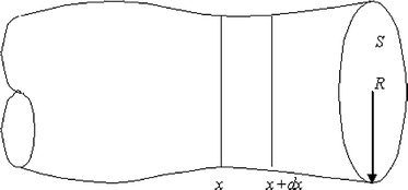
A control volume of an ideal artery between x and x + dx

As seen in Eq. (5), the change of G and R 0 affect the pulse wave velocity c. So pulse wave velocity c is a variable with respect to t and x. In this sense, Eq. (8) is a non-linear partial differential equation. A relationship between PWV and BP can be derived by solving the equation.
Derivation of BP-PWV Function
Wave equation (8) lays a strong foundation in deriving the BP-PWV function. It represents the variation of arterial radius R with respect to time t and position x along axis direction. To solve this equation, the constrained conditions from practical considerations and real applications are listed as below:
-
(1)
Propagation of the starting point of a pulse wave is used to calculate the PWV relative to DBP. From time point of view, within a cardiovascular cycle, the starting point of the aortic pulse wave represents the moment when the aortic valve just starts to open and the heart starts to pump blood into aorta. At this moment, the pressure inside the left ventricle has not been applied to aorta. So the starting point of the aortic pulse wave is considered as the end of diastolic state and not affected by the pressure inside the left ventricle. Besides, propagation of the aortic valves closure point on a pulse wave can be used to calculate the PWV relative to SBP. When the aortic valve starts to close, the heart just finishes pumping blood into aorta and the pressure inside the left ventricle has been completely applied to aorta. After that, the pressure inside aorta is not affected by the pressure inside the left ventricle. So the moment of aortic valves closure can be considered as the end of the systolic state. From these, we can say that at the moment of some characteristic points appear, such as the starting point of a pulse wave and the closure point of aortic valves, there is no external force from the heart applied onto the arterial wall and only elastic stress that comes from the arterial wall exists.
-
(2)
Pulse wave velocity c is a variable that is changing with arterial pressure p. In our research, PWV is considered to be an independent variable which is obtained by measurement as introduced in section “Implementation Methodology.” In real applications, it is difficult to obtain the instantaneous PWV of a particular point inside arterial system. Usually, we use the propagation distance in a unit time to represent PWV, which is just the average velocity in a cardiac cycle. Therefore, velocity c in this paper is a discrete variable with an interval of a cardiac cycle.
-
(3)
The arterial pressure p in this paper refers to SBP or DBP instead of continuous instantaneous pressure. The SBP and DBP are also changing discretely with the period of a cardiac cycle.
-
(4)
Although the PWV, SBP and DBP are all discrete, the relationship between PWV and SBP/DBP is a continuous function.
Now from elastic mechanics, we have
where ε is the strain of arterial wall. Substituting Eq. (9) into (8) gives
According to the relationship of stress σ and strain ε in elastic mechanics, we have
Based on the postulated conditions in the previous section, we ignore the discrepancy of G between different blood vessels and consider it to be invariant along axis direction x. Substituting Eq. (11) into (10), we have:
Let M be the mass of an arbitrary particle on arterial wall. Multiply M on both sides of Eq. (12), yields
As mentioned in the first constrained condition, when SBP or DBP occur, there is only elastic stress that comes from the arterial wall. In consequence, Newton’s second law can be applied. Let s be the area of application of σ, then
Combining Eqs. (13) and (14), we obtain
Suppose that the length of a thin wall and straight artery is L, the thickness of the arterial wall is h, the arterial internal and external radii are r 1 and r 2 respectively. Arterial internal pressure p 1 is balanced with external pressure p 2, and σ can be decomposed into circumferential direction and axial direction. Assume that L dose not change with pressure. Then σ in the axial direction can be ignored and thus σ here only represents the stress in circumferential direction. Figure 2 shows an arbitrary cross section of the artery. Line segment ABCD passes central axis of the artery and the surface where it is located divides this artery section into two parts. Now we consider force equilibrium condition for the upper part. Total circumferential tension applied to the surfaces where AB and CD are located is 2hσL, which are downwards and perpendicular to the surfaces of action. The component of p 1 that is perpendicular to bottom line AOD can be expressed as \( p_{1} \sin \theta .\) Applying curvilinear integral to the upper half of the circumference of the inner circle, we get

An arbitrary cross section of the artery section L
So the total internal force applied to the inside surface of the artery section is 2r 1 Lp 1 directing upwards. In a similar way, the total external force applied to the outside surface of the artery section is downwards and equal to 2r 2 Lp 2. According to the balance condition of force, Oka-Azuma equation is obtained.14
Suppose that h is very small so that it can be ignored, and let r 1 = r 2 = r, we have the Laplace equation
Note that p = p 1 − p 2 is the transmural blood pressure. So Eq. (18) becomes
If we consider the artery wall as a thin-wall cylindrical shell and neglect the geometrical change of arterial vessel, r can be seen as a constant with respect to x. Substituting Eq. (19) into (15), we get
According to the second and third constrained conditions, p refers to the SBP or DBP instead of instantaneous pressure, c is the average PWV in a fixed unit time T, Then c can be expressed as the function of distance x.
Taking partial derivative of c respect to x, we get
Note that
Substituting Eq. (23) into (20), we have
Now there is only one independent variable c in Eq. (24), the partial derivative can be represented by the following ordinary differential equation
Let k = sGT/M, we have
Then
We get
We call Eq. (29) as BP-PWV function for pulse wave. It is a general solution of Eq. (26), which can describe the relationship between BP and PWV. The undetermined coefficient k contains elastic module G, which mostly depends on age and gender. Suppose that there are m different age groups and let i denote one particular group of them. Also using j denotes either male or female. Thus parameters k and b have 2m possible values expressed as:
Once k ij and b ij are determined, a family of specific solutions of the general function (29) can be obtained:
The function family (30) represents the basic mathematical models which can be used to calculate the real time BP. From the mathematical point of view, Eq. (29) has finite number of specific solutions. From the biomedical point of view, Eq. (30) contains physiological information of people with different ages and genders. Determination of unknown coefficient k ij and b ij is a problem of parameter identification. We need some samples of p ij and c ij from different age and gender groups to carry out the identification. The general procedure will be described in the model parameter identification algorithm in the next section.
Implementation Methodology
Pulse Wave Acquisition
Considering that ECG is easily accessible, the most popular way is to acquire the PAT instead of PTT.1,3,4,6,7,9–12,15 But PAT includes pre-ejection period that may introduce large errors to real PTT. To avoid this problem, two pulse waves are acquired using infrared light PPG sensors located at ear and toe in our study. The time interval between some characteristic points on the two pulse waves is the real PTT. Pulse waves are acquired and stored in real time using a data acquisition system developed by us as given in Fig. 3. The detailed design information is presented by Chen et al.2

Experimental setup for pulse wave acquisition
In pulse wave acquisition, human subject protection is an important issue that must be considered. Compared with other methods, infrared light sensor that has been used in measuring oxygen saturation of blood can ensure the safety of human subjects. Because there is no electrical contact between human subjects and the infrared light sensors, and a faint gleam of infrared light has no harmful effect on human body. In addition, infrared light sensor is small and light in weight, which does not bring discomfort to human subjects.
Determination of PWV Relative to DBP
Since the wave length of a pulse wave is longer than its propagation distance, PTT is obtained from the propagation of the same characteristic point from the ear pulse to the toe pulse. The starting point of the ear pulse is corresponding to the lowest BP at aortic arch within a cardiac cycle. During the propagation of the starting point from ear to toe, all arteries on the way are in the lowest diastolic pressure state. Therefore, the PTT of starting point is relative to DBP.2 Identification method of the starting point is illustrated in Fig. 4. Firstly, the points denoting the foot and the maximum gradient of the systolic rising edge of a pulse wave are identified. Then we determine the point showing 60% of the maximum gradient between the foot and max-gradient and draw the tangent line at the point. The staring point is the intersection between this line and the tangent line of the foot of the systolic rising edge. In Fig. 4, points a and b are the starting points of ear pulses and toe pulses respectively. Our experimental studies have verified that this method of identifying the starting point is practically feasible. The criterion on 60% of the maximum gradient is obtained from numerous experimental tests.

Identification of the starting points of ear pulse and toe pulse
In fact, the propagation direction of the pulse wave from aortic arch to ear is opposite to that from aortic arch to toe. Therefore, when we consider the propagation distance, the distance from aortic arch to ear must be subtracted from the distance from aortic arch to toe. The propagation distance divided by PTT gives PWV. The detailed calculation of PWV relative to DBP is given by Chen et al.2
In this paper, only PWV relative to DBP is considered for verifying the feasibility of the modeling methodology. But it may lay a strong foundation for the future study of SBP measurement by PWV.
Reference DBP Acquisition
In our study, the main transmission path of the pulse wave includes carotid arteries, thoracic and abdominal aortas, femoral arteries and big arteries in shank. Thus PWV in application is the average velocity, which has the best correlation with the average DBP of every position in arterial system. But it is too difficult to measure DBP from every position so that calculation of the average DBP of arterial system is impossible. An effective way of reference DBP acquisition is to make use of the DBP measured at a specific position to represent the average DBP in arterial system. Usually, brachial arterial DBP and radial arterial DBP are used as reference BP according to noninvasive and invasive methods respectively.10,11 In our study, the commonly accepted radial arterial pressure is chosen as the reference DBP. This facilitates the model verification according to AAMI standard.
Model Parameter Identification Algorithm and Calibration in Modeling Process
The theoretical BP-PWV model (30) must be calibrated or the model parameters must be identified before it is applied to continuous BP measurement. In previous studies, model calibration is usually done in the process of practical measurement. In our research, in order to avoid individual calibration in practical application, we identify the model parameters or calibrate the model in the process of modeling.
According to the definitions in section “Mathematical Modeling”, we have m different age groups (i.e. i = 1, 2…m) for both gender (i.e. j = 1, 2). For group ij, the algorithm of identifying parameters k ij and b ij is listed as follows:
-
(1)
N (N ≥ 5) volunteers of the same age and gender corresponding to group ij are selected to be subjects investigated. Considering that it is not easy to have many volunteers, the smallest number of N equals 5, which has statistical significance.
-
(2)
Simultaneously record p ij,n and c ij,n data for the nth (n = 1,2 … N) volunteer. p ij,n is beat-to-beat invasive BP, and c ij,n takes the average value of PWV in 8 cardiac cycles in order to cancel the effect of breath. In each trial, at least 10 pair of p ij,n and c ij,n data are recorded.
-
(3)
For the nth volunteer, his/her p ij,n must have some changes. The range of change should satisfy: DBP ≥ 25 mmHg and SBP ≥ 40 mmHg. This is because only the p ij,n and c ij,n of large variation are reliable for model parameter identification.
-
(4)
The ‘cftool’ in Matlab is used to plot the recorded p ij,n and c ij,n of the nth volunteer and do curve fitting using the BP-PWV function (29). A pair of coefficients k ij,n and b ij,n are obtained.
-
(5)
Some cases may cause curve fitting unsuccessful, for examples, the BP variation range of a patient is too small, catheter jam causes irregular invasive p ij,n and sensor displacement results in irregular c ij,n . In these cases, select a new volunteer in group ij, and repeat the 2nd, 3rd and 4th steps above for this volunteer.
-
(6)
After all the N volunteers in group ij are considered, parameters k ij and b ij are obtained by taking the average
$$ b_{ij} = {\frac{1}{N}}\sum\limits_{n = 1}^{N} {b_{ij,n} } \quad {\text{and}}\quad k_{ij} = {\frac{1}{N}}\sum\limits_{n = 1}^{N} {k_{ij,n} } $$ -
(7)
Change the age i or gender j factor and repeat the above steps until the parameter identification is finished for all the groups.
Calibration in modeling process is completed through determining a family of BP-PWV functions by statistical method. The calibrated models are called benchmark models, which form an alternative function base that contains the characteristics of people in different age and gender groups. For a person with fixed age and gender, there always exists a suitable benchmark function that can be used to estimate BP based on the measured PWV. In this way, calibration in practical application is no longer required. This modeling idea is similar to the development of gene information base for disease diagnosis.
Experimental Verification
Experimental Subjects and Conditions
The most persuasive way of model verification is clinical trials. Twenty-three patients with age around 19 and 60 are chosen as experimental subjects, as shown in Table 1. By choosing subjects of study in this way, we can investigate the differences caused by age and gender factors. Study approval was given by the Medical Ethics Committee of Southwest Hospital Chongqing China.
In Table 1, each data set includes one patient’s DBP and PWV values acquired simultaneously in operation rooms. The PWV acquisition device mentioned in section “Pulse Wave Acquisition” was used for real time measuring and recording PWV data. At the same time, patients were undergoing surgical operations in which their radial arteries were cannulated (BD 20-gauge, BD Medical Devices Co) and connected via pressure tubing and transducer (PX 260 Pressure Monitoring Kit, Edward Life sciences LLC) interfaced with a monitor (Patient Monitor Solar 8000M, GE medical Systems Information Technologies Inc) that provided real time invasive DBP. Data acquisition continued for a few hours including the time before, during and after anaesthetic. We compared the PWV of the same DBP in the three time periods and found that there was no obvious difference. It indicates that anesthesia has no significant effect on pulse wave propagation in arterial system. During surgery, patients’ BP often had large variation. In some cases, DBP went beyond 100 mmHg. In certain other cases, such as brain surgery that must be done in low BP condition, DBP needed to be maintained near 50 mmHg. In different situations, we had different ways of DBP recording. When the patients’ DBP changed slowly, data only needed to be recorded in every 5 min. When patients’ BP had fast changes, data should be recorded in every 20–60 s.
DBP-PWV Model Verification of Individual Patients
According to the parameter identification algorithm above, for each subject, curve fitting is done using his/her recorded p ij and c ij data and function (29). Figure 5 shows the curve fitting results of four subjects in different age or gender as examples.

Curve fittings of a (a) 60-year-old male, (b) 58-year-old female, (c) 18-year-old male, and (d) 19-year-old female
It can be observed that the derived BP-PWV function is consistent with the experimental data distributions. Note that parameters b and k take different values for different ages or genders. Besides, the experimental data of the other patients also fall into the feasible domain of their corresponding fitting curves, which are not shown here.
For comparison, Fig. 6 illustrates the curve fitting results of the subject in Fig. 5b using some previously proposed functions and the function derived in this paper. In these functions, p denotes estimated BP, c denotes PWV and p o denotes a constant base level BP. It can be observed that function 3 and 4 could not fit the experiment data well. Both function 1 and 2 fit the experiment data well within the data range.

Comparison of curve fitting results obtained using four different functions
To compare the fitting results of the four functions quantitatively, we compute the summed square of residuals (SSE) and the square of the correlation between the response values and the predicted response values (R-Square) for each subject using cftool in Matlab. The mean SSE and R-Square (across all 23 subjects in section “Experimental Subjects and Conditions”) for each fitting function are reported in the Table 2.
Table 2 shows that the fitting results of our function and the logarithmic function are better than the other two functions, which lead to the same conclusion as that in Fig. 6. But there is no significant difference between the exponential function and the logarithmic function. This is due to the considered data are only DBP values, which just cover a limited range. If we consider a wider range that may include both lower DBP and SBP which are not available in this paper, we expect that our model will give better results. This is qualitatively proved by obtaining limits of the two functions as follows.
For the logarithmic function, p approaches negative infinity when c approaches zero. It indicates that it has a problem to express BP-PWV relationship within low BP range. For our function, the limit of p is zero when c approaches zero, and p converges to a limit when c approaches plus infinity. It is means that our model is a bounded function and always maintains positive, which makes sense in the real condition that BP varies in a positive and limited range.
Model Parameter Identification and Benchmark Model Development
According to the model parameter identification algorithm introduced in the previous section, statistical DBP-PWV functions of age groups 19 and 60 for both genders are obtained based on clinical trial data of patients mentioned in section “Experimental Subjects and Conditions”.
In Fig. 7, M-19.2 and M-60.4 represent male groups of average age 19.2 and 60.4 respectively, while F-19.8 and F-59.7 represent female groups of average age 19.8 and 59.7 respectively. It can be seen that under the same DBP condition PWV of M-60.4 is much faster than M-19.2. And the same conclusion can be drawn for F-59.7 and F-19.8. This is because the elastic modulus of arterial wall increases with age which causes the increase of PWV. The effect of gender can be investigated by comparing PWV of M-19.2 and F-19.8 in the same DBP condition. Obviously, PWV of M-19.2 is faster since the elastic modulus of arterial wall of male is usually larger than that of female at the same age.

Statistical BP-PWV functions of the 19 and 60 age groups
The developed benchmark models can be used to estimate BP for the 19 and 60 age groups. For instance, the benchmark model M-60.4 can be used to estimate the DBP of a male near 60 without individual calibration.
In benchmark models development, there is no restriction for pulse wave acquisition and PWV calculation method. The ways of pulse wave acquisition include ultrasound, plethysmograph, pressure transducers and so on. These methods have different positions of measurement and different distances between sensors. So PWVs determined using different methods may more or less have some discrepancies. Therefore, k ij and b ij obtained from different c ij may have some discrepancies as well. In one word, different signal acquisition methods may be corresponding to different BP-PWV functions. Current researches have not reached a consensus in term of the best way of PWV measurement. Photoelectric plethysmograph is used in our studies.
Clinical Verification of DBP-PWV Benchmark Model
To verify the effectiveness of the developed benchmark models, they are practically used to measure DBP continuously and non-invasively for subjects whose ages are near 19 and 60. Programming was done based on the benchmark models and combined with the PWV measurement device.
Conditions of clinical verification are listed below:
-
(1)
Subjects chosen for clinical verification are different from those samples chosen for benchmark models development
-
(2)
Invasive DBP of subjects are measured under the same conditions in section “Experimental Subjects and Conditions” and used as criterion. The noninvasive DBP measured by PWV method and cuff sphygmomanometer are simultaneous with the reference invasive DBP.
-
(3)
Clinical verification must meet the test standard for electronic sphygmomanometer in ANSI/AAMI SP10, as given in Table 3. According to the test standard, at least 5 set of BP data must be measured in each trial. If the measured data extend 10 sets, the first 10 sets are used. The time interval between two consecutive records ranges from 1 to 10 min.
Table 3 DBP measurement results of two noninvasive methods
Twenty subjects of age round 19 (5 male and 5 female) and 60 (5 male and 5 female) were chosen for clinical verification. According to AAMI standard, their invasive and noninvasive DBP are recorded at 5-min intervals. The sample size for each trail was 10 sets and each set of data includes one invasive DBP value and two noninvasive DBP values. The mean deviation and standard deviation are used as criterions because the error distributions of noninvasive DBP are normal distributions. Detail error calculation method is strictly based on the test standard in ANSI/AAMI SP10. The measurement results are summarized in Table 3.
As shown in Table 3, DBP measurement results by PWV method have met the AAMI test standard, and they are better than that obtained by cuff sphygmomanometer. But the results in our study are only suitable for people who have healthy cardiovascular systems. For those who have pathological angiosclerosis, their PWV should be faster than normal healthy people so that the benchmark model may overestimate their BP. In these cases, individual calibration is required.
Figure 8 illustrates the error distribution of the two noninvasive methods for the 200 sets of data. The two methods give quite different error distribution compared to the invasive one, and both of them have few number of errors going beyond the range of 16 mmHg (two standard deviations), but corresponding to different subjects. In fact, no matter what noninvasive method is used, it is ineluctable that a small quantity of subjects has large error. But their different error distributions are very useful for doctors in clinical condition. For instance, in certain BP measurement, the two noninvasive methods are applied together and the measurement results are compared. If both methods give similar results, it indicates that the noninvasive measurement error for this subject is relatively small and both methods are feasible. But if the measurement results are quite different, it means that one of them has large measurement error. Although it is difficult to determine which method is more accurate in this case, the results may call attention to the doctor to use invasive method in order to avoid medical negligence.

(a) Error distributions of DBP measured using PWV method compared to invasive method. (b) Error distributions of DBP measured using cuff sphygmomanometer comparing to invasive method
For the purpose of allowing readers to get a good sense of long-term DBP measurement, Fig. 9 gives the time courses of the reference invasive DBP and two noninvasive DBP of a 60-year-old man. X axis shows the number of records with maximum of 50. The time interval between two records is 5 min so that the entire time of BP measurement is 4 h and 10 min. In fact, beat-to-beat DBP could be measured by PWV method, but since cuff sphygmomanometer only provided DBP value per 5 min, we record the three DBP values simultaneously at 5-min intervals for better comparison. The time course line of PWV method verges on the line of cuff method in the first 50 min, and locates between the lines of cuff method and invasive method in the next 150 min. In the last 50 min, it approaches to the line of invasive method. This indicates the accuracy of DBP measurement by PWV method falls in between the cuff method and invasive method.

Time courses of the reference invasive DBP and two noninvasive DBP for a 60-year-old man
Conclusions
In this paper, a new BP-PWV model is mathematically derived based on the fundamental laws. From the biomedical point of view, it contains physiological information of people with different ages and genders. We believe that the proposed modeling methodology is sustainable in theory and can be put into practice. To verify the feasibility of this modeling methodology, we developed benchmark models for a few age and gender groups based on clinical data obtained from patients with healthy cardiovascular system. The DBP measurement results using the developed benchmark models have met the test standard in ANSI/AAMI SP10. From the results of clinical verification, we can draw some important conclusions as given below:
-
(1)
The proposed BP-PWV function correctly expresses the BP-PWV relationship. It lays a strong theoretical foundation for continuous and noninvasive BP measurement based on PWV.
-
(2)
The DBP measurement results can meet the requirement of error range in clinical condition. It indicates that the developed benchmark models have medical utility.
-
(3)
The modeling idea in this paper is original and it may blaze a new path in the research area of BP measurement based on PWV. It may become an independent philosophy of noninvasive BP measurement without calibration by other methods such as cuff sphygmomanometer. It is very valuable in clinical application.
References
Chen, W., T. Kobayashi, S. Ichikawa, Y. Takeuchi, and T. Togawa. Continuous estimation of systolic blood pressure using the pulse arrival time and intermittent calibration. Med. Biol. Eng. Comput. 38:569–574, 2000.
Chen, Y., C. Wen, H. Tang, and X. Teng. The relationship between different pulse wave velocity and systolic/diastolic pressure. The 3rd IEEE Conference on Industrial Electronics and Applications, Singapore, 2008.
Chua, C. P., and C. Heneghan. Continuous blood pressure monitoring using ECG and finger photoplethysmogram. The 28th IEEE EMBS Annual International Conference, New York, 2006.
Fung, P., G. Dumont, C. Ries, C. Mott, and M. Ansermino. Continuous noninvasive blood pressure measurement by pulse transit time. The 26th Annual International Conference of the IEEE EMBS, San Francisco, CA, 2004.
Hughes, D. J., C. F. Babbs, L. A. Geddes, and J. D. Bourland. Measurement of Young’s modulus of elasticity of the canine aorta with ultrasound. Ultrason. Imaging 1:356–367, 1979.
Kaniusas, E., H. Pfützner, L. Mehnen, J. Kosel, and J. C. Téllez-Blanco. Method for continuous nondisturbing monitoring of blood pressure by magnetoelastic skin curvature sensor and ECG. IEEE Sens. J. 6:819–828, 2006.
Lass, J., K. Meigas, D. Karai, R. Kattai, J. Kaik, and M. Rossmann. Continuous blood pressure monitoring during exercise using pulse wave transit time measurement. The 26th Annual International Conference of the IEEE EMBS, 2004.
Mei, C. C. Pulse Wave Propagation in Arteries. MIT’s (Massachusetts Institute of Technology) OpenCourseWare, 2004.
Muehlsteff, J., X. L. Aubert, and M. Schuett. Cuffless estimation of systolic blood pressure for short effort bicycle tests: the prominent role of the pre-ejection period. The 28th IEEE EMBS Annual International Conference, New York, 2006.
Poon, C. C. Y., and Y. T. Zhang. Cuff-less and noninvasive measurements of arterial blood pressure by pulse transit time. The 2005 IEEE Engineering in Medicine and Biology 27th Annual Conference, Shanghai, China, 2005.
Poon, C. C. Y., and Y. T. Zhang. The beat-to-beat relationship between pulse transit time and systolic blood pressure. The 5th International Conference on Information Technology and Application in Biomedicine, Shenzhen, China, 2008.
Shaltis, P., A. Reisner, and H. Asada. Calibration of the photoplethysmogram to arterial blood pressure: capabilities and limitations for continuous pressure monitoring. The 2005 IEEE Engineering in Medicine and Biology, Shanghai, China, 2005.
Shi, Y., and N. Deng. Human Circulatory System and Anaesthesiology. Beijing: China Medical Scientific Press, 1990.
Wang, H., and Z. Wen. Mechanics of Blood Circulation, 1990, pp. 83–84, 93–94.
Wong, M. Y. M., C. C. Y. Poon, and Y. T. Zhang. Can the timing-characteristics of phonocardiographic signal be used for cuffless systolic blood pressure estimation? The 28th IEEE EMBS Annual International Conference, New York, 2006.
Zhang, Z. B., and T. H. Wu. The techniques of non-invasive blood pressure measurement and its development. Chin. J. Med. Instrum. 27:196–199, 2003.
Acknowledgments
This work was supported partly by the Southwest hospital of Chongqing in China. The authors are thankful to the staffs in anesthesiology department for facilitating contacts that made this work possible. Also the authors would like to express their sincere appreciation to the reviewers for their constructive comments and suggestions.
Author information
Authors and Affiliations
Corresponding author
Rights and permissions
About this article
Cite this article
Chen, Y., Wen, C., Tao, G. et al. Continuous and Noninvasive Blood Pressure Measurement: A Novel Modeling Methodology of the Relationship Between Blood Pressure and Pulse Wave Velocity. Ann Biomed Eng 37, 2222–2233 (2009). https://doi.org/10.1007/s10439-009-9759-1
Received:
Accepted:
Published:
Issue Date:
DOI: https://doi.org/10.1007/s10439-009-9759-1