Applying FISTA to optimization problems (with or) without minimizers

Abstract

Beck and Teboulle’s FISTA method for finding a minimizer of the sum of two convex functions, one of which has a Lipschitz continuous gradient whereas the other may be nonsmooth, is arguably the most important optimization algorithm of the past decade. While research activity on FISTA has exploded ever since, the mathematically challenging case when the original optimization problem has no minimizer has found only limited attention. In this work, we systematically study FISTA and its variants. We present general results that are applicable, regardless of the existence of minimizers.

1 Introduction

We assume that

(1)

with inner product $\langle \cdot | \cdot \rangle$ and associated norm $||\, \cdot \, ||$. We also presuppose throughout the paper that

(2)

satisfy the following:

Assumption 1.1

(A1):

f is convex and Fréchet differentiable on $\mathcal {H}$, and ${\nabla {f} }$ is $\beta$-Lipschitz continuous with $\beta \in ]0, {+}\infty [$;

(A2):

g is convex, lower semicontinuous, and proper;

(A3):

$\gamma \in ]0,1/\beta ]$ is a parameter.

One fundamental problem in optimization is to

$$\begin{aligned} \text {minimize } f+g \text { over } \mathcal {H}. \end{aligned}$$

(3)

For convenience, we set

(4)

and where we follow standard notation in convex analysis (as employed, e.g., in [8]). Then many algorithms designed for solving (3) employ the forward-backward or proximal gradient operator T in some fashion. Since the advent of Nesterov’s acceleration [22] (when $g\equiv 0$) and Beck and Teboulle’s fast proximal gradient method FISTA [11] (see also [9, Chapter 10]), the literature on algorithms for solving (3) has literally exploded; see, e.g., [1,2,3, 5, 7, 11, 18, 22] for a selection of key contributions. Indeed, out of nearly one million mathematical publications that appeared since 2009 and are indexed by Mathematical Reviews, the 2009-FISTA paper [11] by Beck and Teboulle takes the number two spot! (In passing, we note that it has been cited more than 6,000 times on Google Scholar where it now receives about 3 new citations every day!) The overwhelming majority of these papers assume that the problem (3) has a solution to start with. Complementing and contributing to these analyses, we follow a path less trodden:

The aim of this paper is to study the behaviour of the fast proximal gradient methods (and monotone variants), in the case when the original problem (3) does not necessarily have a solution.

Before we turn to our main results, let us state the FISTA or fast proximal gradient method:

Algorithm 1.2

(FISTA) Let $x_{0} \in \mathcal {H}$, set $y_{1}:=x_{0}$, and update

(5)

where T is defined in (4), $\mathbb {N}^{*}:=\{1,2,\ldots \}$, and $(\tau _n)_{n\in \mathbb {N}^{*}}$ is a sequence of real numbers in $[1,+\infty [$.

Note that when $\tau _n\equiv 1$, one obtains the classical (unaccelerated) proximal gradient method. There are two very popular choices for the sequence $(\tau _n)_{n\in \mathbb {N}^{*}}$ to achieve acceleration. Firstly, given $\tau _1 :=1$, the classical FISTA [10, 11, 16, 22] update is

(6)

The second update has the explicit formula

(7)

where $\rho \in [2, {+}\infty [$; see, e.g., [3, 5, 15, 27].

Convergence results of the sequence generated by FISTA under a suitable tuning of can be found in [1, 5, 15]. The relaxed case was considered in [7] and error-tolerant versions were considered in [2, 3]. In addition, for results concerning the rate of convergence of function values, see [10, 11, 26, 27]. The authors of [16] established a variant of FISTA that covers the strongly convex case. An alternative of the classical proximal gradient algorithm with relaxation and error is presented in [19] (see also [8, 13, 26]). Finally, a new forward-backward splitting scheme (for finding a zero of a sum of two maximally monotone operators) that includes FISTA as a special case was proposed in [18].

The main difference between our work and existing work is that we focus on the minimizing property of the sequences generated by FISTA and MFISTA in the general framework, i.e., when the set is possibly empty. Let us now list our main results:

• Theorem 5.3 establishes the behaviour of FISTA in the possibly inconsistent case; moreover, our assumption on (see (39)) is very mild.

• Theorem 5.5 concerns FISTA when behaves similarly to the Beck–Teboulle choice.

• Theorem 5.10 deals with the case when is bounded; see, in particular, (ii)(a) and (v)(b).

• Theorem 6.1 considers MFISTA [10], the monotone version of FISTA, when Assumption 4.1 is in force and is unbounded.

To the best of our knowledge, Theorem 5.3 is new. The proof of Theorem 5.5, which can be viewed as a “discrete version” of [3, Theorem 2.3], relies on techniques seen in [3, Theorem 2.3] and [1, Proposition 3]; items (ii)–(vi) are new. A result similar to Theorem 5.5(ii) was mentioned in [6, Theorem 4.1]. However, no proof was given, and the parameter sequence there is a special case of the one considered in Theorem 5.5. Items (vii)(a) and (vii)(a) is a slight modification of [4, Proposition 4.3]. Concerning Theorem 5.10, items (i)–(iv) and (v)(b) are new while (v)(a) was proven in [1, Corollary 20(iii)]. Item (i) in the classical case ($\tau _{n} \equiv 1$) relates to [12, Theorem 4.2] where linesearches were employed. In Theorem 6.1, items (i)–(v) are new. Compared to [10, Theorem 5.1], we allow many possible choices for the parameter sequence in Theorem 6.1(vi); see, e.g., Examples 4.4–4.6. In addition, by adapting the technique of [1, Theorem 9], we improve the convergence rate of MFISTA under the condition (110) in Theorem 6.1.

There are also several minor results worth emphasizing: Lemma 2.4 is new. The notion of quasi-Fejér monotonicity is revisited in Lemma 2.7; however, our error sequence need not be positive. The assumptions in Lemma 3.2 and Lemma 3.3 are somewhat minimal, which allow us to establish the minimizing property of FISTA and MFISTA in the case where there are possibly no minimizers in Sects. 5 and 6. Example 4.5 is new. Proposition 5.12 describes the behaviour of in the classical proximal gradient (ISTA) case while Corollary 5.15 provides a sufficient condition for strong convergence of $(x_n)_{n\in \mathbb {N}^{*}}$ in this case. The new Proposition 5.14 presents some progress towards the still open question regarding the convergence of generated by classical FISTA. The weak convergence part in Corollary 5.15 was considered in [4]; however, our new Fejérian approach allows us to obtain strong convergence when .

Let us now turn to the organization of this paper. Classical results on real sequences and new results on the Fejér monotonicity are recorded in Sect. 2. The “one step” behaviour of both FISTA and MFISTA is carefully examined in Sect. 3. In Sect. 4, we investigate properties of the parameter sequence $(\tau _n)_{n\in \mathbb {N}^{*}}$. Our main results on FISTA and MFISTA are presented in Sects. 5 and 6 respectively. The concluding Sect. 7 contains a discussion of open problems.

A final note on notation is in order. For a sequence and an extended real number $\xi \in \left[ {-}\infty , {+}\infty \right]$, the notation $\xi _{n}\uparrow \xi$ means that is increasing (i.e., $\xi _n\leqslant \xi _{n+1}$) and $\xi _{n} \rightarrow \xi$ as $n\rightarrow {+}\infty$. Likewise, $\xi _{n}\downarrow \xi$ means that is decreasing (i.e., $\xi _{n}\geqslant \xi _{n+1}$) and $\xi _{n}\rightarrow \xi$ as $n\rightarrow {+}\infty$. For any other notation not defined, we refer the reader to [8].

2 Auxiliary results

In this section, we collect results on sequences which will make the proofs in later sections more structured.

Lemma 2.1

Let be an increasing sequence in $[1, {+}\infty [$ such that $\lim \tau _{n} = {+}\infty$. Then

(8)

Proof

See Appendix A. $\square$

Lemma 2.2

Let and be sequences in $\mathbb {R}_{+}$. Suppose that $\sum _{n \in \mathbb {N}^{*}}\alpha _{n} = {+}\infty$ and that $\sum _{n \in \mathbb {N}^{*}}\alpha _{n}\beta _{n} < {+}\infty$. Then $\varliminf \beta _{n} =0$.

Proof

See Appendix B. $\square$

The novelty of the following result lies in the fact that the error sequence need not lie in $\mathbb {R}_{+}$.

Lemma 2.3

Let be a sequence in $\mathbb {R}$, let be a sequence in $\mathbb {R}_{+}$, and let be a sequence in $\mathbb {R}$. Suppose that is bounded below, that

(9)

and that the series $\sum _{n \in \mathbb {N}^{*}}\varepsilon _{n}$ converges in $\mathbb {R}$. Then the following hold:

• (i) is convergent in $\mathbb {R}$.

• (ii) $\sum _{n \in \mathbb {N}^{*}}\beta _{n} < {+}\infty$.

Proof

See Appendix C. $\square$

Lemma 2.4

Let be a sequence of real numbers. Consider the following statements:

• (i) converges in $\mathbb {R}$.

• (ii) $\sum _{n \in \mathbb {N}^{*}}\alpha _{n}$ converges in $\mathbb {R}$.

• (iii) converges in $\mathbb {R}$.

Suppose that two of the statements (i)–(iii) hold. Then the remaining one also holds.

Proof

See Appendix D. $\square$

The following result is stated in [25, Problem 2.6.19]; we provide a proof in Appendix E for completeness.

Lemma 2.5

Let be a decreasing sequence in $\mathbb {R}_{+}$. Then

(10)

The following variant of Opial’s lemma [23] will be required in the sequel.

Lemma 2.6

Let C be a nonempty subset of $\mathcal {H}$, and let and be sequences in $\mathcal {H}$. Suppose that $u_{n} - v_{n} \rightarrow 0$, that every weak sequential cluster point of lies in C, and that, for every $c \in C$, converges. Then there exists $w \in C$ such that $u_{n} \rightharpoonup w$ and $v_{n}\rightharpoonup w$.

Proof

For every $c \in C$, since $u_{n}-v_{n}\rightarrow 0$ and converges, we deduce that converges. In turn, because every weak sequential cluster point of belongs to C, [8, Lemma 2.47] yields the existence of $w \in C$ satisfying $v_{n} \rightharpoonup w$. Therefore, because $u_{n}-v_{n}\rightarrow 0$, we conclude that and converge weakly to w. $\square$

We next revisit the notion of quasi-Fejér monotonicity in the Hilbert spaces setting studied in [17]. This plays a crucial role in our analysis of Proposition 5.14. Nevertheless, to fit our framework of Proposition 5.14, the error sequence is not required to be positive in Lemma 2.7. The proof is based on [17, Proposition 3.3(iii) and Proposition 3.10].

Lemma 2.7

Let C be a nonempty subset of $\mathcal {H}$, let be a sequence in $\mathcal {H}$, and let be a sequence in $\mathbb {R}$. Suppose that

(11)

and that $\sum _{n \in \mathbb {N}^{*}}\varepsilon _{n}$ converges in $\mathbb {R}$. Then the following hold:

• (i) For every $c \in C$, the sequence converges in $\mathbb {R}$.

• (ii) Suppose that ${\text {int}}C \ne \varnothing$. Then converges strongly in $\mathcal {H}$.

Proof

• (i): This is a direct consequence of Lemma 2.3(i).

• (ii): We follow along the lines of [17, Proposition 3.10]. Let $v \in {\text {int}}C$ and $\rho \in ]0, {+}\infty [$ be such that . Define a sequence in C via

  

  (12)

We now verify that

(13)

Fix $n \in \mathbb {N}^{*}$. If $u_{n+1}=u_{n}$, then (11) implies that $\varepsilon _{n} \geqslant 0$, and therefore (13) holds. Otherwise, because $v_{n} \in C$, (11) yields $||u_{n+1}-v_{n} ||^{2} \leqslant ||u_{n}-v_{n} ||^{2} +\varepsilon _{n}$. In turn, using (12), we obtain

(14)

and after expanding both sides and simplifying terms, we get (13). Consequently, owing to (13) and the convergence of $\sum _{n \in \mathbb {N}^{*}}\varepsilon _{n}$, we derive from Lemma 2.3(ii) that $\sum _{n \in \mathbb {N}^{*}}2\rho ||u_{n+1}-u_{n} || < {+}\infty$. Hence, by completeness of $\mathcal {H}$, converges strongly to a point in $\mathcal {H}$. $\square$

We conclude this section with a simple identity. If x, y, and z are in $\mathcal {H}$, then

(15)

3 One-step results

The aim of this section is to present several results on performing just one step of FISTA or MFISTA. This allows us to present subsequent convergence results more clearly. Recall that Assumption 1.1 is in force and (see (4)) that

(16)

Clearly,

(17)

Lemma 3.1

(Beck–Teboulle) The following holds:

(18)

Proof

See Appendix F. $\square$

Lemma 3.2

(one FISTA step) Let , let $\tau$ and $\tau _{+}$ be in $[1, {+}\infty [$, and set

(19)

In addition, let $z \in {\text {dom}}{h}$, and set

(20)

Then the following hold:

• (i) .

• (ii) .

• (iii) Suppose that $\tau \leqslant \tau _{+}$, that , and that $\inf h > {-}\infty$. Then

  

  (21)

Proof

First, since $z \in {\text {dom}}{h}$, we get from (17), (19), and (20) that $\mu \in \mathbb {R}$ and $\mu _{+} \in \mathbb {R}$. Next, because $x_{+} = Ty_{+}$, we derive from (18) (applied to ) that

(22)

• (i): We derive from (22), (15), and (19) that

  

  (23a)
  

  (23b)

  and thus, since , the conclusion follows.

• (ii): Since $x_{+} = Ty_{+}$, applying (18) to gives

  

  (24)

  Therefore, because $\tau _{+} -1 \geqslant 0$ by assumption, it follows from (22) and (24) that

  

  (25a)
  

  (25b)
  

  (25c)

  In turn, on the one hand, multiplying both sides of (25) by $\tau _{+} >0$, we infer from (15) (applied to ) and the very definition of $u_{+}$ that

  

  (26a)
  

  (26b)
  

  (26c)

  On the other hand, since due to (19), the definition of u yields

  

  (27)

  Altogether, , which implies the desired conclusion.

• (iii): Since and, by assumption, $\tau _{+}^{2} -\tau _{+} -\tau ^{2} \leqslant 0$, we deduce that . Hence, because $0 < \tau \leqslant \tau _{+}$ and , it follows that . Consequently, (ii) implies that

  

  (28a)
  

  (28b)
  

  (28c)

  as required.$\square$

The analysis of the following lemma follows the lines of [10, Theorem 5.1].

Lemma 3.3

(one MFISTA step). Let , let $\tau$ and $\tau _{+}$ be in $[1, {+}\infty [$, and set

(29)

Furthermore, let $w \in {\text {dom}}h$, and define

(30)

Then the following hold:

• (i) .

• (ii) .

Proof

First, since $z_{+} = Ty_{+}$, using (18) with and (15) with yields

(31a)

(31b)

• (i): On the one hand, by the very definition of $x_{+}$ and (31), , and thus,

  

  (32)

  On the other hand, due to (29),

  

  (33a)
  

  (33b)
  

  (33c)

  and since $\tau \geqslant 1$, it follows that

  $$\begin{aligned} ||y_{+}-x || \leqslant \frac{\tau }{\tau _{+}}||z-x_{-} ||. \end{aligned}$$

  (34)

  Altogether, (32) and (34) yield the desired result.

• (ii): Applying (18) to the pair and noticing that $z_{+} = Ty_{+}$, we get

  

  (35)

In turn, since $\tau _{+}\geqslant 1$, the very definition of $x_{+}$, (31), and (35) imply that

(36a)

(36b)

(36c)

(36d)

(36e)

(36f)

Thus, since $\tau _{+} >0$, it follows from (15) (applied to ) that

(37a)

(37b)

Furthermore, by the definition of $y_{+}$, we have , which asserts that . Combining this and (37) entails that

(38)

which completes the proof. $\square$

4 The parameter sequence

A central ingredient of FISTA and MFISTA is the parameter sequence . In this section, we present various properties of the parameter sequence as well as examples. From this point onwards, we will assume the following:

Assumption 4.1

We assume that is a sequence of real numbers such that

(39)

Remark 4.2

A few observations regarding Assumption 4.1 are in order.

• (i) It is clear from (39) that

  

  (40)

• (ii) Because is increasing,

  $$\begin{aligned} \tau _{n} \uparrow \tau _{\infty } \overset{(40)}{\in } \left[ 1, {+}\infty \right] . \end{aligned}$$

  (41)

• (iii) Due to (40) and the assumption that , it is straightforward to verify that

  

  (42)

• (iv) For every $n \in \mathbb {N}^{*}$, since by (39), it follows from (42) and (40) that

  

  (43)

Lemma 4.3

The following hold:

• (i) $\varlimsup (\tau _n/n)\leqslant \tau _1/2$.

• (ii) Using the convention that $\tfrac{1}{ {+}\infty }= 0$, we have

  

  (44)

• (iii) Suppose that $\lim \tau _{n} = {+}\infty$. Then

  $$\begin{aligned} \lim \frac{\tau _{n}-1}{\tau _{n+1}} = 1. \end{aligned}$$

  (45)

Proof

• (i): We claim that $\tau _n\leqslant \tau _1(n+\sqrt{n})/2$. The inequality is clear when $n=1$. Assume that, for some integer $n\geqslant 1$, we have $\tau _n\leqslant \tau _1(n+\sqrt{n})/2$. Then, on the one hand, we derive from (39) that

  $$\begin{aligned} \tau _{n+1} \leqslant \frac{1+\sqrt{1+4\tau _n^2}}{2} \leqslant \frac{\tau _1+\sqrt{\tau _1^2+\tau _1^2(n+\sqrt{n})^2}}{2} =\frac{\tau _1\big (1+\sqrt{1+(n+\sqrt{n})^2}\big )}{2}. \end{aligned}$$

  (46)

  On the other hand, since $(n+\sqrt{n+1})^2-(1+(n+\sqrt{n})^2) =2n(\sqrt{n+1}-\sqrt{n})>0$, we obtain $\sqrt{1+(n+\sqrt{n})^2}<n+\sqrt{n+1}$. Altogether, $\tau _{n+1}<\tau _1(n+1+\sqrt{n+1})/2$, which concludes the induction argument. Consequently, $\varlimsup (\tau _n/n) \leqslant \lim \tau _1(n+\sqrt{n})/(2n)=\tau _1/2$.

• (ii): First, since by (39), we infer from (41) that . Next, by (42) and (39), we have

  

  (47a)
  

  (47b)
  

  (47c)
  

  (47d)

  and hence, we get from (41) that , as desired.

• (iii): Follows from (ii) and (41).

$\square$

Example 4.4

The condition

$$\begin{aligned} \sup _{n\in \mathbb {N}^{*}} \big (n/\tau _n\big ) <+\infty \end{aligned}$$

(48)

and the quotient

$$\begin{aligned} \frac{\tau _n-1}{\tau _{n+1}} \end{aligned}$$

(49)

play significant roles in subsequent convergence results. Here are the two popular examples of sequences that satisfy Assumption 4.1 as well as (48) already seen in Sect. 1:

• (i) [10, 11, 16, 22] Set $\tau _{1} :=1$, and set . Then, it is straightforward to verify that and that is an increasing sequence in $[1, {+}\infty [$. Moreover, an inductive argument shows that , from which we obtain $\tau _\infty =+\infty$ and . This and Lemma 4.3(i) guarantee that $\lim (\tau _n/n)=1/2$. Furthermore, it is part of the folklore that

  

  (50)

  for completeness, a proof is provided in Appendix G.

• (ii) [3, 5, 15, 27] Let $\rho \in [2, {+}\infty [$, and define . Then, clearly is an increasing sequence in $[1, {+}\infty [$ with $\tau _\infty =+\infty$ and, for every $n \in \mathbb {N}^{*}$, we have ,

  

  (51)

  and

  $$\begin{aligned} \frac{\tau _n-1}{\tau _{n+1}} =\frac{n-1}{n+\rho } =1-\frac{1+\rho }{n}+ {\mathrm {O}}{\bigg (\frac{1}{n^2}\bigg ) }. \end{aligned}$$

  (52)

We now turn to examples of the condition

(53)

which is of some interest in Sect. 5 (see (107)) and Sect. 6. Further examples of sequences that satisfy (53) can be found in [1, Section 5].

Example 4.5

Let $\rho \in \bigl ]1, {+}\infty \bigr [$ and set

(54)

Then

(55)

If , then the sequence satisfies (53) with .

Proof

Indeed, since , we derive from (42), (43), and (54) that

(56a)

(56b)

as claimed. The remaining implication follows readily. $\square$

Example 4.6

[7] Let , set

(57)

and suppose that one of the following holds:

• (i) $d=0$.

• (ii) $d \in ]0,1]$ and .

Aujol and Dossal’s [7, Lemma 3.2] yields

(58)

Let us add to their analysis by pointing out that if (ii) holds, then (53) holds with . Indeed, (57) and (58) assert that

(59)

Also, note that if $d\in ]0,1[$, then (by L’Hôpital’s rule) in contrast to Example 4.4.

5 FISTA

In this section, we present three main results on FISTA. We again recall that Assumption 1.1 is in force and (see (4)) that

(60)

Algorithm 5.1

(FISTA). Let $x_{0} \in \mathcal {H}$, set $y_{1}:=x_{0}$, and update

(61)

where T is as in (60) and satisfies (39).

We assume for the remainder of this section that

(62)

We also set

(63)

Note that, by (39) and (40),

(64)

The first two items of the following result are due to Attouch and Cabot; see [1, Proposition 3].

Lemma 5.2

The following holds:

• (i) .

• (ii) The sequence is decreasing and convergent to a point in $[ {-}\infty , {+}\infty [$.

• (iii) Suppose that $\inf _{n \in \mathbb {N}^{*}} \sigma _{n} > {-}\infty$. Then the following hold:

  • (a) .

  • (b) Suppose that $\sup _{n \in \mathbb {N}^{*}}\tau _{n} < {+}\infty$. Then and $\sum _{n \in \mathbb {N}^{*}} ||x_{n}-x_{n-1} ||^{2} < {+}\infty$.

Proof

• (i): For every $n \in \mathbb {N}^{*}$, Lemma 3.2(i) (applied to ) asserts that , from which the desired inequality follows. (ii): A consequence of (i) and (64).

• (iii)(a): By (i) and (63),

  

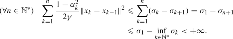  (65)

  Thus, , as claimed.

• (iii)(b): Because the function is increasing and , we see that ; therefore,

  

  (66)

  Combining (66) and (a) yields the conclusion. $\square$

We are ready for our first main result which establishes a minimizing property of the sequence generated by Algorithm 5.1 in the general setting.

Theorem 5.3

The following holds:

(67)

Proof

Let us first establish that

(68)

To do so, we proceed by contradiction: assume that there exists $N\in \mathbb {N}^{*}$ such that . Then, there exists $z \in {\text {dom}}h$ satisfying

(69)

In turn, set . For every $n \geqslant N$, in the light of Lemma 3.2(ii) (applied to ), we get

(70a)

(70b)

Furthermore, due to (69),

(71)

Let us consider the following two possible cases.

• (a) $\tau _{\infty } = {+}\infty$: By (41), $\tau _{n}\rightarrow {+}\infty$. Next, we derive from (42), (70) and (71) that or, equivalently, by the very definition of ,

  

  (72)

  Consequently, since $\tau _{n} \uparrow {+}\infty$, taking the limit superior in (72) gives , which contradicts (69).

• (b) $\tau _{\infty } < {+}\infty$: Set . Then, by (71), and, by (42) and (69), . In turn, on the one hand, combining (70) and Lemma 2.3(ii), we infer that . On the other hand, because and by our assumption and (40),

  

  (73)

from which we deduce that . Altogether, Lemma 2.2 and (71) guarantee that , i.e., . Consequently, due to the inequality , it follows from (69) that , which is absurd.

To summarize, we have reached a contradiction in each case, and therefore (68) holds. Thus, because as $n\rightarrow {+}\infty$, we infer from (68) that as $n\rightarrow {+}\infty$. Finally, (68) guarantees that , which completes the proof. $\square$

Remark 5.4

In Theorem 5.3, we do not know whether or not converges to $\inf h$. However, Theorem 5.5, Theorem 5.10, and Proposition 5.8 suggest a positive answer.

We are now ready for our second main result (Theorem 5.5), which is a discrete version of Attouch et al.’s [3, Theorem 2.3]. When is as in Example 4.4(ii) with $\rho =2$, items (ii) and (iv) were mentioned (without a detailed proof) in [6, Theorem 4.1]. The analysis of Theorem 5.5(iii) was motivated by Attouch and Cabot’s [1, Proposition 3]. Furthermore, the boundedness of the sequences and in the consistent case was first obtained in Attouch et al.’s [4, Proposition 4.3]; here, we slightly modified the proof of this result to obtain the boundedness of in a more general setting.

Theorem 5.5

Suppose that

(74)

For every $z \in {\text {dom}}h$, set . Then the following hold:

• (i) For every $z \in {\text {dom}}{h}$, we have

  

  (75)

  and

  

  (76)

• (ii) .

• (iii) is asymptotically regular, i.e., $x_{n} - x_{n-1} \rightarrow 0$.

• (iv) Every weak sequential cluster point of belongs to ${{\,\mathrm{Argmin}\,}}{h}$.

• (v) Suppose that has a bounded subsequence. Then ${{\,\mathrm{Argmin}\,}}{h} \ne \varnothing$.

• (vi) Suppose that ${{\,\mathrm{Argmin}\,}}{h} = \varnothing$. Then $||x_{n} || \rightarrow +\infty$.

• (vii) Suppose that ${{\,\mathrm{Argmin}\,}}{h} \ne \varnothing$. Then the following hold:

  • (a) (Beck–Teboulle [11]) as $n\rightarrow {+}\infty$; more precisely, for every $z \in {{\,\mathrm{Argmin}\,}}h$,

    

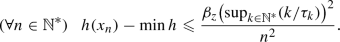    (77)

  • (b) The sequences and are bounded.

Proof

Set . Since , we see that

$$\begin{aligned} \tau _{n} \rightarrow +\infty . \end{aligned}$$

(78)

• (i): Take $z \in {\text {dom}}{h}$, and set

  

  (79)

  Now, for every $n \in \mathbb {N}^{*}$, since $\inf {h} > -\infty$, $\tau _{n} \leqslant \tau _{n+1},$ and , applying Lemma 3.2(iii) to yields . Hence, because is increasing and , an inductive argument gives

  

  (80a)
  

  (80b)
  

  (80c)

  Therefore, since (75) trivially holds when $n=1$, we obtain the conclusion. Consequently, (76) readily follows from (75).

• (ii): For every $z \in {\text {dom}}{h}$, taking the limit superior over n in (76) and using (78) yields . Consequently, letting , we conclude that , as desired.

• (iii): First, due to (63), , and thus,

  $$\begin{aligned} \inf _{n \in \mathbb {N}^{*}}\sigma _{n} > {-}\infty . \end{aligned}$$

  (81)

  Hence, we conclude via Lemma 5.2(ii) that is convergent in $\mathbb {R}$. In turn, on the one hand, (ii) and (63) imply that

  

  (82)

  On the other hand, (81) and Lemma 5.2(a) yield , and since due to Lemma 2.1 and (78), we get from Lemma 2.2 that

  $$\begin{aligned} \varliminf ||x_{n}-x_{n-1} ||^{2} = 0. \end{aligned}$$

  (83)

  Altogether, combining (82) and (83) yields $x_{n}-x_{n-1}\rightarrow 0$, as announced.

• (iv): Let x be a weak sequential cluster point of , say $x_{k_{n}}\rightharpoonup x$. Then, since h is convex and lower semicontinuous, it is weakly sequentially lower semicontinuous by [8, Theorem 9.1]. Hence, (ii) entails that , which ensures that $x \in {{\,\mathrm{Argmin}\,}}{h}$.

• (v): Combine (iv) and [8, Lemma 2.45].

• (vi): This is the contrapositive of (v).

• (vii)(a): Clear from (i) and (74).

• (vii)(b): Fix $z \in {{\,\mathrm{Argmin}\,}}h$. For every $n \geqslant 2$, because , we derive from (75) that

  

  (84)

and now a simple expansion gives

(85a)

(85b)

(85c)

(85d)

(85e)

(85f)

(85g)

In turn,

(86)

Hence, since and , we get

(87)

from which the boundedness of follows. Consequently, because and both sequences on the right-hand side are bounded due to (84) and (87), we conclude that is bounded, as announced. $\square$

Remark 5.6

By choosing the sequence as in Example 4.4(i), we shall see in Proposition 5.8 that Theorem 5.5(ii) is still valid even when the assumption that $\inf {h}> - \infty$ is omitted. Therefore, it is appealing to conjecture that this assumption can be left out in Theorem 5.5(ii). In stark contrast, it is crucial to assume that h is bounded from below in Theorem 5.5(iii), as illustrated in Example 5.7.

Example 5.7

Suppose that $\mathcal {H}= \mathbb {R}$, that $f :\mathcal {H}\rightarrow \mathbb {R}: x \mapsto -x$, that $g = 0$, that $\gamma =1$, and that $\tau _{n}\uparrow \tau _\infty = {+}\infty$. Then, since ${{\text {Prox}}_{g}} = {\text {Id}}$ and , we see that (61) turns into

(88)

Hence, , and upon setting , we obtain

(89)

Let us establish that $z_{n} \rightarrow {+}\infty .$ First, since $y_{1}=x_{0}$ by Algorithm 5.1, we get from (88) that $z_{1} =x_{1}-x_{0} = x_{1}-y_{1} = 1$. In turn, by induction and (89), . We now suppose to the contrary that $\xi :=\varliminf z_{n} \in \mathbb {R}_{+}$. Then, taking the limit inferior over n in (89) and using Lemma 4.3 yield $\xi = 1 + 1\cdot \xi = 1 + \xi$, which is absurd. Therefore, $\xi = {+}\infty$, and it follows that $x_{n} - x_{n-1} = z_{n}\rightarrow {+}\infty$.

Proposition 5.8

Suppose that the sequence is as in Example 4.4(i). Then .

Proof

First, as seen in Example 4.4(i),

(90)

Now it is sufficient to show that . To do so, fix $z \in {\text {dom}}{h}$, and set . Then, according to Lemma 3.2(ii) and (90),

(91)

Thus,

(92)

Hence, because $\lim \tau _{n} = +\infty$, taking the limit superior over n yields . Consequently, since z is an arbitrary element of ${\text {dom}}{h}$, we conclude that , as required. $\square$

Remark 5.9

Proposition 5.8 is a special case of the accelerated inexact forward-backward splitting developed in [28]; see [28, Theorem 4.3 and Remark 3].

We now turn to our third main result, which concerns the case where the parameter sequence in Assumption 4.1 is bounded.

Theorem 5.10

Suppose that $\tau _{\infty } < {+}\infty$. Then the following hold:

• (i) .

• (ii) Assume that $\inf h > {-}\infty$. Then the following hold:

  • (a) $\sum _{n \in \mathbb {N}^{*}}||x_{n}-x_{n-1} ||^{2} < {+}\infty$.

  • (b) Every weak sequential cluster point of lies in ${{\,\mathrm{Argmin}\,}}h$.

• (iii) Assume that has a bounded subsequence. Then ${{\,\mathrm{Argmin}\,}}h \ne \varnothing$.

• (iv) Assume that ${{\,\mathrm{Argmin}\,}}h = \varnothing$. Then $||x_{n} || \rightarrow {+}\infty$.

• (v) Assume that ${{\,\mathrm{Argmin}\,}}h \ne \varnothing$. Then the following hold:

  • (a) (Attouch–Cabot [1]) as $n\rightarrow {+}\infty$.

  • (b) $\sum _{n \in \mathbb {N}^{*}}n ||x_{n}-x_{n-1} ||^{2} < {+}\infty .$ As a consequence, .

Proof

• (i): Since, by (63), and, by Lemma 5.2(ii), converges to a point $\sigma \in [ {-}\infty , {+}\infty [$, it is enough to verify that $\sigma = \lim \sigma _{n} = \inf h$. Assume to the contrary that

  $$\begin{aligned} {-}\infty \leqslant \inf h< \sigma . \end{aligned}$$

  (93)

  It then follows that $\inf _{n \in \mathbb {N}^{*}}\sigma _{n} > {-}\infty$, and Lemma 5.2(b) thus yields $||x_{n}-x_{n-1} ||^{2} \rightarrow 0$, from which and (63) we deduce that . This and Theorem 5.3 imply that $\sigma = \inf h$. This and (93) yield a contradiction.

• (ii)(a): Our assumption ensures that $\inf _{n \in \mathbb {N}^{*}}\sigma _{n} > {-}\infty$, and therefore, thanks to the boundedness of , Lemma 5.2(b) yields $\sum _{n \in \mathbb {N}^{*}}||x_{n}-x_{n-1} ||^{2} < {+}\infty$.

• (ii)(b), (iii), and (iv): Similar to Theorem 5.5(iv), (v), and (vi), respectively.

• (v): Fix $z \in {{\,\mathrm{Argmin}\,}}h$, and set . By (41), we have

  $$\begin{aligned} \tau _{n} \uparrow \tau _{\infty }, \end{aligned}$$

  (94)

  which implies that $\tau _{n}^{2} - \tau _{n+1}^{2}+\tau _{n+1} \rightarrow \tau _{\infty }$. Therefore, because $\tau _{\infty }\in ]0, {+}\infty [$, there exists $N \in \mathbb {N}^{*}$ such that

  

  (95)

  Next, for every $n \geqslant N$, using Lemma 3.2(ii) with , we get . Hence, because and, by (42), , Lemma 2.3(ii) and (95) give . This, (ii)(a), and (63) ensure that

  

  (96)

  Furthermore, Lemma 5.2(ii) and (i) yield

  $$\begin{aligned} \sigma _{n}-\min h \downarrow 0. \end{aligned}$$

  (97)

• (v)(a): Appealing to (96) and (97), Lemma 2.5 guarantees that . Consequently, since , the conclusion follows.

• (v)(b): Thanks to (96) and (97), we derive from Lemma 2.5 that

  

  (98)

  and hence, by Lemma 5.2(i), . Thus, because due to the boundedness of and Lemma 5.2(b), we conclude that $\sum _{n \in \mathbb {N}^{*}}n ||x_{n}-x_{n-1} ||^{2} < {+}\infty$. This gives $n||x_{n}-x_{n-1} ||^{2} \rightarrow 0$, i.e., as $n\rightarrow {+}\infty$, as desired.

$\square$

Remark 5.11

• (i) In the case of the classical forward-backward algorithm (without the extrapolation step) with linesearches, results similar to Theorem 5.10(i) and (iv) were established in [12, Theorem 4.2] by Bello Cruz and Nghia. To the best of our knowledge, Theorem 5.10(i) is new in the setting of Algorithm 5.1.

• (ii) Theorem 5.10(v)(a) was obtained by Attouch and Cabot [1, Corollary 20(iii)]. Here we provide a proof based on the technique developed in [1] to be self-contained.

• (iii) The summabilities established in Theorem 5.10(ii)(a) and (v)(b) are new. Nevertheless, in the case of the forward-backward algorithm, i.e., when $\tau _{n} \equiv 1$, Theorem 5.10(v)(b) appears implicitly in the Beck and Teboulle’s proof of [11, Theorem 3.1].

In the case of the classical forward-backward algorithm, by applying [14, Corollary 1.5] to the forward-backward operator , we obtain further information on the sequence as follows.

Proposition 5.12

Suppose that , and set¹$^{,}$². Then $x_{n}- x_{n-1}\rightarrow v$.

Proof

By assumption, Algorithm 5.1 becomes . Next, we learn from [21, Proposition 3.2 and Corollary 4.2] that T is averaged, i.e., there exists $\alpha \in ]0,1 [$ and a nonexpansive operator $R :\mathcal {H}\rightarrow \mathcal {H}$ such that . Hence, we conclude via [14, Proposition 1.3 and Corollary 1.5] that $x_{n} - x_{n-1} = T^{n}x_{0} - T^{n-1}x_{0} \rightarrow v$. For an alternative proof of [14, Corollary 1.2] in the Hilbert space setting, see [21, Proposition 2.1]. $\square$

Remark 5.13

Some comments are in order.

• (i) In stark contrast to Proposition 5.12 and Theorem 5.10, if $\tau _{\infty }= {+}\infty$, then it may happen that $||x_{n}-x_{n-1} || \rightarrow {+}\infty$ (see Example 5.7).

• (ii) For a recent study on the forward-backward operator T, we refer the reader to [21].

Proposition 5.14

Suppose that ${{\,\mathrm{Argmin}\,}}h\ne \varnothing$, that converges in $\mathbb {R}$, and that $\tau _{n}||x_{n}-x_{n-1} || \rightarrow 0$. Then the following hold:

• (i) .

• (ii) The sequence converges weakly to a point in ${{\,\mathrm{Argmin}\,}}h$.

• (iii) Suppose that . Then converges strongly to a point in ${{\,\mathrm{Argmin}\,}}h$.

Proof

Set

(99)

Since, by (40) and (99), and since, by our assumption, $\tau _{n}||x_{n}-x_{n-1} || \rightarrow 0$, we see that

$$\begin{aligned} z_{n}-x_{n}\rightarrow 0. \end{aligned}$$

(100)

Next, due to our assumption and

(101a)

(101b)

we see that

$$\begin{aligned} \sum _{n \in \mathbb {N}^{*}}\varepsilon _{n} ~\text {is convergent in } \mathbb {R}. \end{aligned}$$

(102)

Let us now establish that

(103)

Fix $z \in {{\,\mathrm{Argmin}\,}}h$ and $n \in \mathbb {N}^{*}$. Applying Lemma 3.2(ii) to and invoking (42) yields

(104a)

(104b)

from which and (99) we obtain (103).

• (i): Since, by assumption, converges and since, by (41), converges in $\mathbb {R}$, it follows that is convergent in $\mathbb {R}$. Therefore, due to Theorem 5.3, .

• (ii): In the light of (i), arguing similarly to the proof of Theorem 5.5(iv), we conclude that

  

  (105)

  In turn, appealing to (102) and (103), Lemma 2.7(i) implies that

  

  (106)

  Thus, combining (100), (105), and (106), we get via Lemma 2.6 that converges weakly to a point in ${{\,\mathrm{Argmin}\,}}h$.

• (iii): Since , owing to Lemma 2.7(ii), we derive from (102) and (103) that there exists $z \in \mathcal {H}$ such that $z_{n } \rightarrow z$. Hence, by (100), $x_{n}\rightarrow z$, and (ii) implies that $z \in {{\,\mathrm{Argmin}\,}}h$. To sum up, converges strongly to a minimizer of h.

$\square$

Corollary 5.15

Suppose that ${{\,\mathrm{Argmin}\,}}h \ne \varnothing$ and that $\sup _{n \in \mathbb {N}^{*}}\tau _{n} < {+}\infty$. Then converges weakly to a point in ${{\,\mathrm{Argmin}\,}}h$. Moreover, if , then the convergence is strong.

Proof

By Theorem 5.10(v), we see that and $||x_{n}-x_{n-1} || \rightarrow 0$, and since $\sup _{n \in \mathbb {N}^{*}}\tau _{n} < {+}\infty$, it follows that and $\tau _{n}||x_{n}-x_{n-1} || \rightarrow 0$. The conclusion thus follows from Proposition 5.14. $\square$

Remark 5.16

Consider the setting of Corollary 5.15. Although the weak convergence of the sequence has been shown in [1, Corollary 20(iv)], our Fejér-based proof here is new and may suggest other approaches to tackle the convergence of in the setting Theorem 5.5(vii).

We conclude this section with an instance where the assumption of Proposition 5.14 holds.

Example 5.17

Suppose, in addition to Assumption 4.1, that there exists $\delta \in ]0,1 [$ such that

(107)

(see Examples 4.5 and 4.6). Then Attouch and Cabot’s [1, Theorem 9] yields and $\tau _{n}||x_{n}-x_{n-1} || \rightarrow 0$.

6 MFISTA

In this section, we discuss the minimizing property of the sequence generated by MFISTA. The monotonicity of function values allows us to overcome the issue stated in Remark 5.4. Compared to Beck and Teboulle’s [10, Theorem 5.1] (see also [9, Theorem 10.40]), we allow other possibilities for the choice of in Theorem 6.1(vi). Furthermore, we provide in item (vii), which was motivated by [1, Theorem 9], a better rate of convergence.

Theorem 6.1

In addition to Assumption 4.1, suppose that $\tau _{\infty }= {+}\infty$. Let $x_{0} \in \mathcal {H}$, set $y_{1}:=x_{0}$, and update

(108)

where T is as in (16). Furthermore, set

(109)

Then the following hold:

• (i) is decreasing and .

• (ii) is decreasing and $\sigma _{n} \downarrow \inf h$.

• (iii) Suppose that $\inf h > {-}\infty$. Then $z_{n} - x_{n-1}\rightarrow 0$ and $x_{n}-x_{n-1}\rightarrow 0$.

• (iv) Suppose that has a bounded subsequence. Then ${{\,\mathrm{Argmin}\,}}h \ne \varnothing$.

• (v) Suppose that ${{\,\mathrm{Argmin}\,}}h = \varnothing .$ Then $||x_{n} || \rightarrow {+}\infty$.

• (vi) Suppose that ${{\,\mathrm{Argmin}\,}}h \ne \varnothing .$ Then as $n\rightarrow {+}\infty$.

• (vii) Suppose that ${{\,\mathrm{Argmin}\,}}h\ne \varnothing$ and that there exists $\delta \in ]0,1[$ such that

  $$\begin{aligned} (\forall n\in \mathbb {N}^{*})\quad \tau _{n+1}^{2}-\tau _n^2\leqslant \delta \tau _{n+1}. \end{aligned}$$

  (110)

  Then

  

  (111)

  and

  

  (112)

Proof

• (i): By (108), the sequence is decreasing, from which we have . Therefore, it suffices to prove that . To this end, assume to the contrary that . This yields the existence of a point $w \in {\text {dom}}h$ such that

  

  (113)

  Set

  

  (114)

  In turn, for every $n \in \mathbb {N}^{*}$, because, by (42), and, by (113), $\mu _{n}> 0$, it follows from Lemma 3.3(ii) (applied to ) that

  

  (115)

  Hence,

  

  (116)

  Consequently, since and $\tau _{n}\rightarrow {+}\infty$, we derive from (116) that , which contradicts (113).

• (ii): Let us first show that is decreasing. Towards this end, for every $n\in \mathbb {N}^{*}$, we deduce from Lemma 3.3(i) that . Therefore,

  

  (117)

  and because , we conclude that

  

  (118)

  It remains to show that $\sigma _{n}\rightarrow \inf h$. Set $\sigma :=\inf _{n \in \mathbb {N}^{*}}\sigma _{n}$. Due to (118),

  $$\begin{aligned} \sigma _{n}\downarrow \sigma \end{aligned}$$

  (119)

  and it therefore suffices to prove that $\sigma = \inf h$. Let us argue by contradiction: assume that $\sigma > \inf h \geqslant {-}\infty$. By (117),

  

  (120)

  which implies that . Thus, since by Lemma 2.1, Lemma 2.2 guarantees that $\varliminf ||z_{n}-x_{n-1} ||^{2} =0$, i.e., $\varliminf ||z_{n}-x_{n-1} || = 0$. In turn, let be a strictly increasing sequence in $\mathbb {N}^{*}$ such that $||z_{k_{n}} - x_{k_{n}-1} || \rightarrow \varliminf ||z_{n}-x_{n-1} ||= 0$. It follows from (i) and (119) that . Consequently, $\sigma =\inf h$, which violates the assumption that $\sigma > \inf h$. To summarize, we have shown that $\sigma _{n}\downarrow \inf h$.

• (iii): Since $\inf h > {-}\infty$, combining (i), (ii), and (109) gives $z_{n} -x_{n-1} \rightarrow 0$. To show that $x_{n}-x_{n-1}\rightarrow 0$, we infer from (108) that, for every $n \in \mathbb {N}^{*}$, $x_{n}-x_{n-1}=x_{n-1}-x_{n-1} = 0$ if , and $x_{n}-x_{n-1} = z_{n}-x_{n-1}$ otherwise; therefore, . Consequently, because $z_{n}-x_{n-1}\rightarrow 0$, it follows that $x_{n}-x_{n-1}\rightarrow 0$, as required.

• (iv) and (v): Straightforward.

• (vi): Fix $w \in {{\,\mathrm{Argmin}\,}}h$ and define . Due to (42) and the fact that , Lemma 3.3(ii) entails that . Hence,

  

  (121)

  which verifies the claim.

• (vii): Let us adapt the notation of (vi). Since $\{\mu _{n}\}_{n\in \mathbb {N}^{*}}\subseteq \mathbb {R}_{+}$, we derive from Lemma 3.3(ii) and (110) that

  $$\begin{aligned}&(\forall n\in \mathbb {N}^{*})\quad \tau _{n+1}^2\mu _{n+1}+(2\gamma )^{-1}||u_{n+1} ||^{2}\nonumber \\&\quad \leqslant \tau _{n+1}(\tau _{n+1}-1)\mu _{n}+(2\gamma )^{-1}||u_{n} ||^{2} \end{aligned}$$

  (122a)
  $$\begin{aligned}&\quad =\tau _{n}^{2}\mu _{n}+(2\gamma )^{-1}||u_{n} ||^{2} -\big (\tau _{n}^{2}-\tau _{n+1}^{2}+\tau _{n+1}\big )\mu _{n} \end{aligned}$$

  (122b)
  $$\begin{aligned}&\quad \leqslant \tau _{n}^{2}\mu _n+(2\gamma )^{-1}||u_{n} ||^{2} -(1-\delta )\tau _{n+1}\mu _n. \end{aligned}$$

  (122c)

On the other hand, since $\delta \in ]0,1[$ and $\{\mu _n\}_{n\in \mathbb {N}^{*}}\subseteq \mathbb {R}_{+}$, it follows that $\{(1-\delta )\tau _{n+1}\mu _n\}_{n\in \mathbb {N}^{*}}\subseteq \mathbb {R}_{+}$. Combining this, (122), and Lemma 2.3(ii), we infer that $(1-\delta )\sum _{n\in \mathbb {N}^{*}}\tau _{n+1}\mu _n< {+}\infty$. In turn, since $(\tau _n)_{n\in \mathbb {N}^{*}}$ is increasing and $1-\delta >0$, it follows that $\sum _{n\in \mathbb {N}^{*}}\tau _{n}\mu _n< {+}\infty$. Consequently, since $(\mu _n)_{n\in \mathbb {N}^{*}}$ is decreasing due to (i) and since clearly $\sum _{n\in \mathbb {N}^{*}}\tau _{n}= {+}\infty$, [1, Lemma 22] ensures that

(123)

which establishes (111). In turn, we deduce from (110), (123), and (i) that

$$\begin{aligned} 0\leqslant \tau _{n+1}^2(h(x_{n+1})-\min h)&=(h(x_{n+1})-\min h)\bigg (\tau _{1}^2+ \sum _{k=1}^{n}\big (\tau _{k+1}^{2}-\tau _{k}^2\big )\bigg ) \end{aligned}$$

(124a)

$$\begin{aligned}&\leqslant (h(x_{n+1})-\min h)\bigg (\tau _{1}^{2}+\delta \sum _{k=1}^{n}\tau _{k+1}\bigg ) \end{aligned}$$

(124b)

$$\begin{aligned}&\leqslant (h(x_{n+1})-\min h)\bigg (\tau _{1}^{2} -\delta \tau _1 +\delta \sum _{k=1}^{n+1}\tau _{k}\bigg ) \end{aligned}$$

(124c)

$$\begin{aligned}&\quad \rightarrow 0\text { as }n\rightarrow {+}\infty , \end{aligned}$$

(124d)

which verifies (112). $\square$

Remark 6.2

In Theorem 6.1, the assumption that $\tau _{\infty }= {+}\infty$ is actually not needed in items (i) and (iv)–(vii). For clarity, let us sketch the proof of (i) under the assumption that $\tau _\infty < {+}\infty$. Assume that $\tau _\infty < {+}\infty$. We infer from the first inequality in (115) that

$$\begin{aligned} (\forall n\in \mathbb {N}^{*})\quad \tau _{n+1}^2\mu _{n+1}+(2\gamma )^{-1}||u_{n+1} ||^2&\leqslant \tau _n^2\mu _n+(2\gamma )^{-1}||u_n ||^2 \nonumber \\&\quad -\big (\tau _n^2-\tau _{n+1}^2+\tau _{n+1}\big )\mu _n \end{aligned}$$

(125)

and it follows from Lemma 2.3(ii) that $\sum _{n\in \mathbb {N}^{*}}(\tau _n^2-\tau _{n+1}^2+\tau _{n+1}) \mu _n< {+}\infty$. One may argue similarly to the case (b) in the proof of Theorem 5.3 to obtain $\varliminf \mu _n=0$ or, equivalently, $\varliminf h(x_n) =h(w)$, which contradicts (113). Therefore $\inf _{n\in \mathbb {N}^{*}}h(x_n)=\inf h$ and we get $h(x_n)\downarrow \inf _{n\in \mathbb {N}^{*}}h(x_n)=\inf h$. Items (iv) and (v) follow from this. In addition, note that we did not use the assumption that $\tau _\infty = {+}\infty$ in the proof of (vi) and (vii). It is, however, worth pointing out that the conclusion of Theorem 6.1(vi) is not so interesting when $\tau _{\infty }< {+}\infty$.

7 Open problems

We conclude this paper with a few open problems.

P1:

In Theorem 5.3, is it true that ?

P2:

What can be said about the conclusions of Theorem 5.5(iii) and (vii)(b) if ?

P2:

Suppose that ${{\,\mathrm{Argmin}\,}}h \ne \varnothing$. Do the sequences generated by Algorithm 5.1 and (108) always converge weakly to a point in ${{\,\mathrm{Argmin}\,}}h$?

Appendices

Appendices

1.1 Appendix A

For the sake of completeness, we provide the following proof of Lemma 2.1 based on [20, Problem 3.2.43].

Proof of Lemma 2.1

Because due to the assumption that , it is sufficient to establish that

(126)

Indeed, since $\tau _{n}\rightarrow {+}\infty$, there exists $N \in \mathbb {N}^{*}$ such that

(127)

Now, set , and . Then, on the one hand, since is increasing and positive, we have , and is therefore an increasing sequence in $\mathbb {R}_{+}$; moreover, due to (127), . On the other hand, because $\tau _{n}\rightarrow {+}\infty$, we have $\sigma _{n} =\tau _{n+1}^{2}-\tau _{1}^{2} \rightarrow {+}\infty$. Altogether, since

(128)

by the fact that is increasing, we see that . It follows that the partial sums of do not satisfy the Cauchy property. Hence, since , we obtain

$$\begin{aligned} \sum _{n \geqslant N}\frac{\tau _{n+1}^{2}-\tau _{n}^{2}}{\tau _{n+1}^{2}-\tau _{1}^{2}} = \sum _{n \geqslant N}\frac{\xi _{n}}{\sigma _{n}} = {+}\infty . \end{aligned}$$

(129)

Consequently, in the light of (127),

(130)

and (126) follows. $\square$

1.2 Appendix B

Proof of Lemma 2.2

Let us argue by contradiction. Towards this goal, assume that $\varliminf \beta _{n} \in ] 0, {+}\infty ]$ and fix $\beta \in ] 0 , \varliminf \beta _{n} [$. Then, there exists $N \in \mathbb {N}^{*}$ such that , and hence, because , we have , it follows that $\sum _{n \geqslant N}\alpha _{n}\beta _{n} \geqslant \sum _{n \geqslant N} \beta \alpha _{n} = {+}\infty$, which violates our assumption. To sum up, $\varliminf \beta _{n} = 0$. $\square$

1.3 Appendix C

The following self-contained proof of Lemma 2.3 follows [17, Lemma 3.1] in the case $\chi =1$; however, we do not require the error sequence to be positive.

Proof of Lemma 2.3

• (i): Set $\alpha :=\varliminf _{n}\alpha _{n} \in \left[ \inf _{n \in \mathbb {N}^{*}}\alpha _{n}, {+}\infty \right]$ and let be a subsequence of that converges to $\alpha$. We first show that $\alpha < {+}\infty$. Since , it follows from (9) that . Thus, ; in particular, . Hence, since $\alpha _{k_{n}}\rightarrow \alpha$ and $\sum _{n \in \mathbb {N}^{*}}\varepsilon _{n}$ converges, it follows that $\alpha \leqslant \alpha _{1} + \sum _{k \in \mathbb {N}}\varepsilon _{k } < {+}\infty$, as claimed. In turn, to establish the convergence of , it suffices to verify that $\varlimsup _{n}\alpha _{n} \leqslant \varliminf _{n} \alpha _{n}$. Towards this goal, let $\delta$ be in $]0, {+}\infty [$. Then, on the one hand, Cauchy’s criterion ensures the existence of $k_{n_{0}} \in \mathbb {N}^{*}$ such that $\alpha _{k_{n_{0} } } - \alpha \leqslant \delta /2$ and that . On the other hand, because , (9) implies that . Altogether, , from which we deduce that $\varlimsup _{n} \alpha _{n} \leqslant \alpha + \delta$. Consequently, since $\delta$ is arbitrarily chosen in $]0, {+}\infty [$, it follows that $\varlimsup _{n}\alpha _{n} \leqslant \alpha = \varliminf _{n}\alpha _{n}$, and therefore, converges to $\alpha$.

• (ii): We derive from (9) that . Hence, since $\sum _{n \in \mathbb {N}^{*}}\varepsilon _{n}$ is convergent and, by (i), $\lim _{n}\alpha _{n} =\alpha$, letting $N \rightarrow {+}\infty$ yields $\sum _{n \in \mathbb {N}} \beta _{n} \leqslant \alpha _{1} - \alpha + \sum _{n \in \mathbb {N}}\varepsilon _{n } < {+}\infty$, and so $\sum _{n \in \mathbb {N}^{*}}\beta _{n} < {+}\infty$, as required.

$\square$

1.4 Appendix D

Proof of Lemma 2.4

Indeed, since

(131a)

(131b)

we readily obtain the conclusion. $\square$

1.5 Appendix E

Proof of Lemma 2.5

“$\Rightarrow$”: Since is a decreasing sequence in $\mathbb {R}_{+}$ and $\sum _{n \in \mathbb {N}^{*}}\alpha _{n} < {+}\infty$, it follows that $n\alpha _{n}\rightarrow 0$ (see, e.g., [20, Problem 3.2.35]). Invoking the assumption that $\sum _{n \in \mathbb {N}^{*}}\alpha _{n} < {+}\infty$ once more, we infer from Lemma 2.4 that , as desired.

“$\Leftarrow$”: A consequence of Lemma 2.4. $\square$

1.6 Appendix F

Proof of Lemma 3.1

This is similar to the one found in [11, Lemma 2.3] and included for completeness; see also [15, Lemma 3.1]. Fix . On the one hand, by (A1) and (A3) in Assumption 1.1, ${\nabla {f} }$ is Lipschitz continuous with constant $\gamma ^{-1}$, from which, the Descent Lemma (see, e.g., [8, Lemma 2.64]), and the convexity of f we infer that

(132a)

(132b)

(132c)

On the other hand, because , [8, Proposition 12.26] asserts that

(133a)

(133b)

Altogether, upon adding (132) and (133), it follows that

(134a)

(134b)

(134c)

which yields (18). $\square$

1.7 Appendix G

Proof of (50)

Recall that $\lim (\tau _n/n)=1/2$. In turn, because $(\forall n\in \mathbb {N}^{*})$ $\tau _n^2=\tau _{n+1}^2-\tau _{n+1}$, it follows that

$$\begin{aligned} \frac{n(\tau _n-\tau _{n+1})}{\tau _{n+1}}= & {} \frac{n(\tau _n^2-\tau _{n+1}^2)}{\tau _{n+1}(\tau _n+\tau _{n+1})} =\frac{-n\tau _{n+1}}{\tau _{n+1}(\tau _n+\tau _{n+1})}\nonumber \\= & {} \frac{-1}{\displaystyle \frac{\tau _n}{n}+\frac{\tau _{n+1}}{n+1}\frac{n+1}{n}} \rightarrow \frac{-1}{\frac{1}{2}+\frac{1}{2}}=-1 \end{aligned}$$

(135)

and therefore that

$$\begin{aligned} n\Bigg (\frac{\tau _n-1}{\tau _{n+1}}-1+\frac{3}{n}\Bigg ) =\frac{n(\tau _n-\tau _{n+1})}{\tau _{n+1}} -\frac{n+1}{\tau _{n+1}}\frac{n}{n+1}+3 \rightarrow -1-2+3=0. \end{aligned}$$

(136)

Hence, (50) holds. $\square$

References

Attouch, H., Cabot, A.: Convergence rates of inertial forward-backward algorithms. SIAM J. Optim. 28, 849–874 (2018)
Attouch, H., Cabot, A., Chbani, Z., Riahi, H.: Inertial forward-backward algorithms with perturbations: application to Tikhonov regularization. J. Optim. Theory Appl. 179, 1–36 (2018)
Attouch, H., Chbani, Z., Peypouquet, J., Redont, P.: Fast convergence of inertial dynamics and algorithms with asymptotic vanishing viscosity. Math. Program. Ser. B 168, 123–175 (2018)
Attouch, H., Chbani, Z., Riahi, H.: Rate of convergence of the Nesterov accelerated gradient method in the subcritical case \(\alpha \le 3\). ESAIM Control Optim. Calc. Var. (2019). https://doi.org/10.1051/cocv/2017083
Attouch, H., Peypouquet, J.: The rate of convergence of Nesterov’s accelerated forward-backward method is actually faster than \(1/k^2\). SIAM J. Optim. 26, 1824–1834 (2016)
Attouch, H., Peypouquet, J., Redont, P.: Fast convergence of an inertial gradient-like system with vanishing viscosity. (2015) arXiv:1507.04782
Aujol, J.-F., Dossal, C.: Stability of over-relaxations for the forward-backward algorithm, application to FISTA. SIAM J. Optim. 25, 2408–2433 (2015)
Bauschke, H.H., Combettes, P.L.: Convex Analysis and Monotone Operator Theory in Hilbert Spaces, second edn. Springer, New York (2017)
Beck, A.: First-Order Methods in Optimization. SIAM, Philadelphia (2017)
Beck, A., Teboulle, M.: Fast gradient-based algorithms for constrained total variation image denoising and deblurring problems. IEEE Trans. Image Process. 18, 2419–2434 (2009)
Beck, A., Teboulle, M.: A fast iterative shrinkage-thresholding algorithm for linear inverse problem. SIAM J. Imaging Sci. 2, 183–202 (2009)
Bello Cruz, J.Y., Nghia, T.T.A.: On the convergence of the forward-backward splitting method with linesearches. Optim. Methods Softw. 31, 1209–1238 (2016)
Bredies, K.: A forward-backward splitting algorithm for the minimization of non-smooth convex functionals in Banach space. Inverse Probl. 25, 015005 (2009)
Bruck, R.E., Reich, S.: Nonexpansive projections and resolvents of accretive operators in Banach spaces. Houst. J. Math. 3, 459–470 (1977)
Chambolle, A., Dossal, C.: On the convergence of the iterates of the “fast iterative shrinkage/thresholding algorithm”. J. Optim. Theory Appl. 166, 968–982 (2015)
Chambolle, A., Pock, T.: An introduction to continuous optimization for imaging. Acta Numer. 25, 161–319 (2016)
Combettes, P.L.: Quasi-Fejérian analysis of some optimization algorithms. In: Butnariu, D., Censor, Y., Reich, S. (eds.) Inherently Parallel Algorithms in Feasibility and Optimization and Their Applications, vol. 8, pp. 115–152. North-Holland, Amsterdam (2001)
Combettes, P.L., Glaudin, L.E.: Quasinonexpansive iterations on the affine hull of orbits: from Mann’s mean value algorithm to inertial methods. SIAM J. Optim. 27, 2356–2380 (2017)
Combettes, P.L., Salzo, S., Villa, S.: Consistent learning by composite proximal thresholding. Math. Program. Ser. B 167, 99–127 (2018)
Kaczor, W.J., Nowak, M.T.: Problems in Mathematical Analysis. I. Real Numbers, Sequences and Series. American Mathematical Society, Providence, RI (2000)
Moursi, W.M.: The forward-backward algorithm and the normal problem. J. Optim. Theory Appl. 176, 605–624 (2018)
Nesterov, Y.E.: A method for solving the convex programming problem with convergence rate \(O(1/k^{2})\). Dokl. Akad. Nauk 269, 543–547 (1983)
Opial, Z.: Weak convergence of the sequence of successive approximations for nonexpansive mappings. Bull. Am. Math. Soc. 73, 591–597 (1967)
Pazy, A.: Asymptotic behavior of contractions in Hilbert space. Israel J. Math. 9, 235–240 (1971)
Rǎdulescu, T.-L., Rǎdulescu, V.D., Andreescu, T.: Problems in Real Analysis: Advanced Calculus on the Real Axis. Springer, New York (2009)
Schmidt, M., Roux, N.L., Bach, F.: Convergence rates of inexact proximal-gradient methods for convex optimization. In: Shawe-Taylor, J., Zemel, R.S., Bartlett, P.L., Pereira, F., Weinberger, K.Q. (eds.) Advances in Neural Information Processing Systems 24, pp. 1458–1466. Curran Associates Inc., Red Hook (2011)
Su, W., Boyd, S., Candès, E.J.: A differential equation for modeling Nesterov’s accelerated gradient method: theory and insights. J. Mach. Learn. Res. 17, 1–43 (2016)
Villa, S., Salzo, S., Baldassarre, L., Verri, A.: Accelerated and inexact forward-backward algorithms. SIAM J. Optim. 23, 1607–1633 (2013)
Acknowledgements
We thank two referees for their very careful reading and constructive comments. HHB and XW were partially supported by NSERC Discovery Grants while MNB was partially supported by a Mitacs Globalink Graduate Fellowship Award.
Author information
Authors and Affiliations
Corresponding author
Additional information
Publisher's Note
Springer Nature remains neutral with regard to jurisdictional claims in published maps and institutional affiliations.