Calculation of Double-Quantum-Coherence Two-dimensional Spectra: Distance Measurements and Orientational Correlations

Abstract

The double-quantum-coherence (DQC) echo signal for two coupled nitroxides separated by distances ≳10 Å, is calculated rigorously for the six-pulse sequence. Successive application of six pulses on the initial density matrix, with appropriate inter-pulse time evolution and coherence pathway selection leaves only the coherent pathways of interest. The amplitude of the echo signal following the last π pulse can be used to obtain a one-dimensional (1D) dipolar spectrum (Pake doublet), and the echo envelope can be used to construct the 2D DQC spectrum. The calculations are carried out using the product space spanned by the two electron-spin magnetic quantum numbers m ₁, m ₂ and the two nuclear-spin magnetic quantum numbers M ₁, M ₂, describing, e.g. two coupled nitroxides in bilabeled proteins. The density matrix is subjected to a cascade of unitary transformations taking into account dipolar and electron exchange interactions during each pulse and during the evolution in the absence of a pulse. The unitary transformations use the eigensystem of the effective spin Hamiltonians obtained by numerical matrix diagonalization. Simulations are carried out for a range of dipolar interactions, D, and microwave magnetic field strength B ₁ for both fixed and random orientations of the two ¹⁴N (and ¹⁵N) nitroxides. Relaxation effects were not included. Several examples of 1D and 2D Fourier transforms of the time-domain signals versus dipolar evolution and spin-echo envelope time variables are shown for illustration. Comparisons are made between 1D rigorous simulations and analytical approximations. The rigorous simulations presented here provide insights into DQC electron spin resonance spectroscopy, they serve as a standard to evaluate the results of approximate theories, and they can be employed to plan future DQC experiments.

1 Introduction

The first theoretical analysis of double-quantum-coherence (DQC) spectra was undertaken by Saxena and Freed [1]. They briefly summarized results for a constant-time six-pulse DQC sequence, but focused instead on a “forbidden” DQC five-pulse sequence. In fact, it is the six-pulse sequence, and not the five-pulse sequence of that type, which has proved to be most useful in distance measurements [2–5]. While the equations in Ref. [1] are generally correct, their prediction that the “allowed” DQC signals would be very weak, have been contradicted by the strong DQC signals obtained in many experimental studies and their analysis [2–5]. It is presumed that there were undetected problems with the numerical simulations.

When a sample containing bilabeled proteins is subjected to a sufficiently strong microwave pulse, the nitroxide electron spin resonance (ESR) spectrum is almost uniformly excited, so that any orientational selection is largely suppressed, that is, it does not modify the echo amplitude (except for the effect of pseudosecular dipolar terms, essential for short distances). Also, as we show, in high B ₁-fields (B ₁ ≳ 2D), the effect of dipolar coupling during the pulses becomes relatively weak. Therefore, for not very short distances and in sufficiently strong B ₁s, the information on orientations of the magnetic tensors of the spin-label moieties, is virtually excluded from the time-domain dipolar evolution of the echo amplitude, taken at its maximum. However, as we show, it is still retained in the spin-echo envelope and can be retrieved by recording the two-dimensional (2D) time-domain data as a function of the spin-echo time (t _echo) and the dipolar evolution time (t _dip) and then converting it into a 2D-Fourier transform (FT) spectrum, which, after making a “shear” transformation [6], separates the dipolar dimension from the spectral dimension. Rigorous computations of 1D and 2D signals have been carried out and are presented here. Efficient but approximate analytical expressions to this end were developed for 1D signals by Borbat and Freed [2] (cf. Appendix 3), who omitted the dipolar coupling during the pulses and assumed an ideal DQ filter. Whereas such expressions are quite useful for practical purposes and computationally very efficient, these approximations may not be generally valid, especially in the case of short distances (e.g. <15.0 Å). In order to test the nature and extent of deviations from the exact results and to establish the scope of applicability, numerical simulations of 1D spectra were carried out rigorously using the new codes developed for 2D computations. Unlike [1], the pulse propagators are calculated, using highly accurate numerical diagonalizations of the Hamiltonians involved, rather than applying a Trotter expansion [7, 8]. Although the computational approach is necessarily time-consuming, it does provide deeper insights into the features of DQC spectroscopy.

2 Theoretical Background

The pulse pattern and the relevant coherence pathways for the six-pulse DQC sequence are shown in Fig. 1 [2, 3]. The method used to compute the 2D-DQC spectra is outlined as follows.

Fig. 1

In this diagram a shows the six-pulse DQC sequence. The coherence pathways in b correspond with the pulses shown in a in that a transition from one p state to another p state is generated by a pulse; the horizontal lines show coherence orders during the evolutions in the absence of a pulse. As for the timing between the various pulses the following is noted. The time interval t ₁ = t ₂ = t _p is increased in equal steps, Δt _p , typically ranging from 1 to 10 ns, over a period of t _m  = t _p  + t ₅ (200–4000 ns in this paper). The time between the t ₃ = t ₄ = t _DQ is kept fixed, typically at 20 ns; t ₅ = t ₆ is stepped by −Δt _p to maintain a constant t _m . It starts from the initial time t _m . The echo envelope is recorded in a window t _w  ~ 80–160 ns, centered at a time delay 2t _m  + 2t _DQ after the first pulse, i.e. at about t ₆ = t _m after the sixth pulse. Note that the width of the echo sampling window limits the minimal values of t ₆ and t _p by about t _w /2 and their maximum values to t _m  − t _w /2. The dipolar evolution is recorded as a symmetric signal with respect to t _dip ≡ t _m  − 2t _p over the range of ±t _m in steps of 2Δt _p . t _dip = 0 when pulse separations are t ₁ = t ₂ = t ₅. In practice t _p starts with t _p0 (~400 ns in this paper), so that the last pulse and the echo window do not overlap. Therefore, the signal in 2D DQC experiment is recorded (or computed) over ±(t _m  − t _p0) with t _p0 always greater than t _w /2

The initial density matrix operator in thermal equilibrium for the two nitroxides described by the static spin Hamiltonian $\hat{H}$ is:

$$ \hat{\rho }_{ 0} = {\frac{{\exp ( - \hat{H}_{0} /kT)}}{{Tr[\exp ( - \hat{H}_{0} /kT)]}}} \propto \hat{S}_{1z} + \hat{S}_{2z} , $$

where the z-axis is defined to be aligned along the direction of the external magnetic field, and the subscripts number the two electron spins. The time evolution of the spin density matrix, $\hat{\rho}$(t), is governed by the Liouville–von Neumann equation [1]:

$$ {\frac{{{\text{d}}\hat{\rho }}}{{{\text{d}}t}}} = - {\frac{i}{\hbar }}{\hat{\hat{H}}}(t)\hat{\rho }(t) - \hat{\hat{\Upgamma }}(\hat{\rho }(t) - \hat{\rho }(0)), $$

where $\hat{\hat{H}}{\hat\rho} \equiv [\hat{H},{\hat\rho} ]$, ħ is Plank’s constant divided by 2π, $\hat{\hat{\Upgamma }}$ is the relaxation operator, i ² = −1. Neglecting the relaxation, the density matrix evolves under the action of $\hat{H}$ as:

$$ {\frac{{{\text{d}}{\hat\rho} }}{{{\text{d}}t}}} = - {\frac{i}{\hbar }}[\hat{H}(t),{\hat\rho} (t)]. $$

Thus after a period of time Δt the density matrix, ρ(t), becomes:

$$ {\hat\rho} (t + \Updelta t) = {\text{e}}^{{ - {\frac{{i\hat{H}\Updelta t}}{\hbar }}}} {\hat\rho} (t){\text{e}}^{{{\frac{{i\hat{H}\Updelta t}}{\hbar }}}} \equiv \hat{U}(\hat{H},\Updelta t){\hat\rho} (t) .$$

(1)

A numerical implementation of Eq. 1 to compute the DQC ESR signal is outlined below. Note that in the sequel the Hamiltonians will be expressed in angular frequency units. In the ensuing for convenience we will drop the carets of $\hat{H}$ and $\hat{\rho}$, which mark them as operators in Hilbert space.

3 Computation of Echo Signal

One starts with the (unnormalized) initial density matrix in thermal equilibrium:

$$ \rho (0) \propto S_{1z} + S_{2z}^{{}}. $$

(2)

for the two coupled nitroxides, with electron spins S _k  = 1/2 (normalization will be performed at the end of the calculation). The six-pulse sequence, as shown in Fig. 1, transforms the initial density matrix under the successive action of six-pulse propagators $R_{k} \;(k = 1,2, \ldots ,6),$ due to the pulses, and six subsequent free-evolution propagators $Q_{k} \;(k = 1,2, \ldots ,6)$. This sequence can be defined as follows:

$$ \begin{gathered} R_{1} \left( {{\frac{\pi }{2}}} \right) \to Q_{1} (t_{p} ) \to R_{2} (\pi ) \to Q_{2} ( t{}_{p}) \to R_{3} \left( {{\frac{\pi }{2}}} \right) \to Q_{3} (t_{\text{DQ}} ) \to R_{4} (\pi ) \to Q_{4} (t_{\text{DQ}} ) \hfill \\ \to R_{5} \left( {{\frac{\pi }{2}}} \right) \to Q_{5} (t_{m} - t_{p} ) \to R_{6} (\pi ) \to Q_{6} (t_{m} - t_{p} + t_{\text{echo}} ), \hfill \\ \end{gathered} $$

(3)

The 12 time evolution periods described by Eq. 3 lead to the density matrix in the final form ρ _f . This is calculated as follows. A kth pulse, applied at the time t and acting during the period of time, τ _k , in the frame of reference rotating with the angular frequency of the circular component of microwave magnetic field resonant with Larmor frequency of the nitroxide electron spin, transforms the density matrix, ρ(t), according to:

$$ \rho (t + \tau_{k} ) = {\text{e}}^{{ - i{H}_{k} \tau_{ki} }} \rho (t){\text{e}}^{{i{H}_{k} \tau_{ki} }} $$

or in the notation of Eq. 3,

$$ \rho (t)\xrightarrow{{R_{k} }}\rho (t + \tau_{k} ) $$

with R _k being the kth pulse propagator due to the effective Hamiltonian H _k acting during the period of time τ _k . The action of a π-pulse can change the sign of a coherence order, p, and the π/2 pulse can generate other coherence orders [9, 10]. In order to follow the pathways of interest, the density matrix is then projected onto the coherence pathways p _k , which are chosen after the pulse according to Fig. 1, as follows:

$$ \rho '(t + \tau_{k} ) = P({\mathbf{p}}_{k} )\rho (t + \tau_{k} ), $$

(4)

where the idempotent operator $P({\mathbf{p}}_{k} )$ projects the density matrix on the coherence pathways p _k chosen after the kth pulse. As shown in Fig. 1, the coherence pathways of interest are [(1, −1); (−1, 1); (2, −2); (−2, 2); (1); (−1)] after the actions of the six pulses, with two branching points leading to a total of four distinct pathways. The subsequent free evolution during the time t _k transforms $\rho^{\prime}(t + \tau_{k} )$ as $\rho^{\prime}(t + \tau_{k} )\xrightarrow{{Q(t_{k} )}}\rho (t + \tau_{k} + t_{k} )$ according to:

$$ \rho (t + \tau_{k} + t_{k} ) = {\text{e}}^{{ - i{{H}} t_{k} }} \rho '(t + \tau_{k} ){\text{e}}^{{i{{H}} t_{k} }} $$

(5)

where H is the spin Hamiltonian in the absence of a pulse. The density matrix $\rho (t + \tau_{k} + t_{k} )$ is then used in place of ρ(t) in Eq. 4 for the calculation of the density matrix under the action of the (k + 1)-pulse, and the steps defined by Eqs. 4 and 5 are repeated to arrive at the final density matrix $\rho_{f} \equiv \rho \left( {\sum\limits_{k} {(\tau_{k} + t_{k} )} } \right)$. Computed in this way, the final density matrix thus becomes a function of several arguments, $\rho_{f} = \rho ({\varvec{\uptau}},{\mathbf{t}},{\mathbf{p}},t{}_{\text{echo}},\eta ,\lambda_{1} ,\lambda_{2} )$. The arguments are as follows: ${\varvec{\uptau}} = (\tau_{1} , \ldots ,\tau_{6} )$ are the pulse durations; ${\mathbf{t}} = (t_{1} , \ldots ,t_{6} )$ are the subsequent free-evolution periods; ${\mathbf{p}} = ({\mathbf{p}}_{1} , \ldots ,{\mathbf{p}}_{6} )$ are the relevant coherence orders during the evolution periods; t _k , t _echo are time variables used to record the dipolar evolution and to produce the spin-echo envelope. The remaining arguments are the Euler angles η = (χ, θ, φ), which define in the laboratory frame the orientation of the vector r connecting the magnetic dipoles associated with the electron spins; and in this dipolar (molecular) frame, whose z-axis is coincident with r, the Euler angles $\lambda_{k} = (\alpha_{k} ,\beta_{k} ,\gamma_{k}^{{}} )$ define the principal axis of the nitroxide magnetic tensors (Fig. 2) with α ₁ chosen to be 0. (The angle χ was set to zero as is appropriate for isotropic media.) Finally, the complex echo signal is given by:

$$ F_{ + } = - 2{\text{Tr}}[S_{ + } \tilde{\rho }_{f} ], $$

where $\tilde{\rho }_{f}$ is the normalized density matrix.

Fig. 2

Set of Euler angles λ _k  = (α _k , β _k , γ _k ), (k = 1, 2), which define the orientations of the hyperfine and g-tensor tensor principal axes for nitroxides 1 and 2 in the dipolar (molecular) frame of reference. In this frame the z-axis is chosen to coincide with the vector r, connecting the magnetic dipoles of the nitroxides. The orientation of the dipolar frame in the laboratory frame (with the z-axis parallel to the external magnetic field B ₀) is defined by the Euler angles η = (0, θ, φ)

The evolution thus depends on the exact form of various propagators that is given by H ₀ in the absence of a pulse or H ₀ + H _p in the presence of a pulse. Appropriate pulse time intervals τ _k are chosen to achieve nominal flip angles of π/2 (k = 1, 3, 5) and π (k = 2, 4, 6), respectively. Here,

$$ H_{0} = H_{01} + H_{02} + H_{12} $$

(6)

with

$$ H_{0k} = S_{kz} {\mathbf{g}}_{k} \cdot {\mathbf{B}}_{0} - \gamma_{n} I_{kz} B_{0} + S_{kz} {\mathbf{A}}_{k} \cdot {\mathbf{I}}_{k}^{{}} $$

(7)

for k = 1, 2 denoting nitroxides 1 and 2 and H ₁₂ giving their coupling

$$ H_{12} = H_{D} + H_{J} = {\frac{D}{2}}(3\cos^{2} \theta - 1)\left( {S_{z}^{2} - {\frac{1}{3}}{\mathbf{S}}^{2} } \right) + J\left( {{\frac{1}{2}} - 2{\mathbf{S}}_{1} \cdot {\mathbf{S}}_{2} } \right). $$

(8)

Here J is the electron exchange constant and D is the dipolar coupling constant

$$ D = {\frac{{3\gamma_{e}^{2} \hbar^{{}} }}{{2r^{3} }}}, $$

(9)

where γ _e is the gyromagnetic ratio for an electron, h is the Plank’s constant, and r is the distance between the nitroxide’s magnetic dipoles separated by r and considered in the point dipole approximation. (The dipolar constant d = 2D/3 will most often be used throughout the text.) In Eq. 7, I _1,2 are the nuclear spins of the nitrogen (¹⁴N or ¹⁵N) nuclei on the two nitroxides.

The interaction with the radiation field due to the applied microwave pulse k in the reference frame rotating with the carrier frequency ω _rf (that is usually set at or near the Larmor frequency) is given by:

$$ H_{pk} = {\frac{{\gamma_{e} B_{1k} }}{2}}({\text{e}}^{{ - i\chi_{k} }} S_{ + } + {\text{e}}^{{i\chi_{k} }} S_{ - } ); $$

(10)

where B _1k is the amplitude of the circular magnetic component of the kth pulse. The phases, χ _k , can be set to zero for all the pulses for purposes of the present calculations and consequently $H_{pk} = \gamma_{e} B_{1k} S_{x}$. The amplitudes, B _1k , do not have to be equal for different k’s, but we will show results for the simplest case of equal amplitudes. H _0k (cf. Appendix 1) can be written in the laboratory frame as

$$ H_{0k} = C_{k} S_{kz} + G_{k} I_{kz} + A_{k} S_{kz} I_{kz} + B_{k} S_{kz} I_{k + } + B_{k}^{*} S_{kz} I_{k - } $$

The 2D time-domain DQC signal is calculated for a given set of λ _k and η, using appropriate variations of the time intervals following the various pulses, as given in the legend to Fig. 1 for typical values used for simulation. The calculations were carried out in the product space $S_{1} \otimes S_{2} \otimes I_{1} \otimes I_{2}$ with the dimension $N = (2S_{1} + 1)(2S_{2} + 1)(2I_{1} + 1)(2I_{2} + 1)$ (or using those generated by subspace permutations, as needed). H ₀ and H are represented by order N × N matrices H ₀ and H, i.e. with the size of 36 × 36 for the two coupled (¹⁴N) nitroxides (S _1,2 = 1/2, I _1,2 = 1). H ₀, not including H ₁₂, can be conveniently diagonalized in the product space $S_{1} \otimes I_{1} \otimes S_{2} \otimes I_{2}$ by the unitary transformation

$$ {\mathbf{T}} = ({\mathbf{S}}_{1\alpha } \otimes {\mathbf{T}}_{1\alpha } + {\mathbf{S}}_{1\beta } \otimes {\mathbf{T}}_{1\beta } ) \otimes ({\mathbf{S}}_{2\alpha } \otimes {\mathbf{T}}_{2\alpha } + {\mathbf{S}}_{2\beta } \otimes {\mathbf{T}}_{2\beta } ), $$

wherein ${\mathbf{S}}_{k\alpha } ,\;{\mathbf{S}}_{k\beta }$ are the matrices representing polarization operators for spin 1/2 and ${\mathbf{T}}_{k\alpha } ,\;{\mathbf{T}}_{k\beta }$ are dimension (2I _k  + 1) unitary matrices diagonalizing the respective nuclear manifolds, α and β. The transformation, however, brings ${\mathbf{S}}_{kx} = {\mathbf{S}}_{x} \otimes {\mathbf{1}}_{{I_{k} }}$ to the form, which contains off-diagonal elements in transformed ${\mathbf{1}}_{{I_{k} }}$s.

$$ {\mathbf{S}}_{kx} = \left( {\begin{array}{*{20}l} 0 & {{\mathbf{M}}_{k}^{{}} } \\ {{\mathbf{M}}_{k}^{{\text{\dag }}} } & 0 \\ \end{array} } \right), $$

where ${\mathbf{M}}_{k} = {\mathbf{T}}_{k\alpha }^{{\text{\dag }}} {\mathbf{T}}_{k\beta }$. If nuclear Zeeman terms can be neglected, as is appropriate for nitroxides in magnetic fields of up to about 12 kG, which corresponds to Q-band, ${\mathbf{M}}_{k} = {\mathbf{1}}_{{I_{k} }}$. In this case both H ₁ and H ₁₂ become block-diagonal in $I_{1} \otimes I_{2} \otimes S_{1} \otimes S_{2}$ with (2I ₁ + 1)(2I ₂ + 1) blocks, corresponding to order 4 × 4 $S_{1} \otimes S_{2}$ electronic subspace. This block-diagonal form makes computations run significantly faster. At higher fields nuclear Zeeman terms should be retained, leading to coupling between nuclear and electron coherences and a large increase in computation time. The procedure to calculate $\rho_{f} (t_{\text{dip}} ,t_{\text{echo}} ,\theta ,\varphi )$ is outlined in Appendix 2. Finally, the complex echo signal is given by:

$$ F_{ + } (t_{\text{dip}} ,t_{\text{echo}} ,\theta ,\varphi ) = - 2{\text{Tr}}[S_{ + } \rho_{f} (t_{\text{dip}} ,t_{\text{echo}} ,\theta ,\varphi )]/{\text{Tr}}[{\mathbf{1}}_{N} ]. $$

where 1 _N is the unity matrix in the product space. The echo signal from a powder (or macroscopically aligned) sample is the average of the signals over the orientations of the molecule in the laboratory frame:

$$ S(t_{\text{dip}} ,t_{\text{echo}} ) = \int\limits_{0}^{2\pi } {{\text{d}}\varphi \int\limits_{0}^{\pi } {F_{ + } (t_{\text{dip}} ,t_{\text{echo}} ,\theta ,\varphi )P_{\Upomega } \sin \theta \,{\text{d}}\theta } } . $$

(11)

Here P _Ω is the angular distribution of molecular axes in the laboratory frame (P _Ω = 1/4π for an isotropic distribution). In performing powder averaging in isotropic medium it suffices to set the integration limits to [0, π] in axial angles and [0, π/2] in polar angles. (Anisotropic media will require averaging over all three Euler angles in η.) When needed, averaging over some or all of the remaining Euler angles, λ _k , and over distances can be conducted.

4 Computational Efficiency and Features

The 1D and 2D simulations based on block-diagonal approximations (i.e. after neglecting the nuclear Zeeman terms in H ₀) were carried out with a typical personal computer using a software code written in MATLAB. In a magnetic field of 6200 G (corresponding to Ku band) the outcome was virtually indistinguishable from that produced by the most rigorous simulations, and the examples we show were produced in this way. Powder averaging employed averaging over the grid on a unit sphere (actually over an octant), but also was carried out on the basis of Monte Carlo averaging. 2D simulations used typically 400 × 80 points in the time-domain, a 180 × 90 point (or greater) grid in {cosθ, φ} or {θ, φ}, or else 1–4 × 10⁴ Monte Carlo trials. For 1D simulations, the grids can be significantly larger. The grid in θ (or cosθ) was spiral or else randomized within the Δθ (or Δcosθ) limits on every step in φ. Grids were constructed for the cosines or the angles for the other polar angles, β _k . The MATLAB code is general enough to permit averaging over any subset of Euler angles or indeed over all of them whether in mesh mode or in Monte Carlo averaging. Averaging was also carried out with respect to the dipolar constant using suitable distance distributions, P(r). The Monte Carlo mode also included angular-dependent inhomogeneous broadening. The last two features are the most practical for 1D computation. A typical computation time for 2D simulations is about 1–2 h, but could be as long as 10 h for very precise results that require the largest meshes noted above or for long Monte Carlo averaging (e.g. when d is large or the distribution in d is broad). A very precise 1D simulation requires some 10–50 min, whereas 1D simulations based on using the expressions from Ref. [2] run about 200 times faster and 10⁵ Monte Carlo trials could typically be used.

The full-scale simulations operating on 36 × 36 matrices were carried out using necessarily a parallel mode with eight 64-bit nodes. The code was written in FORTRAN 77 and built for Linux OS using a Portland Group FORTRAN compiler and Open MP. A 64 × 45-point grid on the unit sphere and 400 × 40 points in time-domain were typical. The mesh used was uniform in cosθ and φ. On average, for a mesh of this size, computation time was about 15 h. However, by using homotopy [11–16] and adaptive meshes, one can hope for a considerable reduction in computation time. Attempts are currently underway to accomplish this.

5 Illustrative Examples

The following examples are chosen to illustrate the calculations.

• 1. Figure 3 displays 1D time-domain results [5] for the dipolar interaction of d = 15 MHz (corresponding to 5.3 G), representing the distance of 15.1 Å between the two ¹⁴N nitroxides, with B ₁ = 30 G, and B ₀ = 6200 G. The Fourier transforms are also included, which shows the respective Pake doublets. The uncorrelated case was simulated using a Monte Carlo method with random angles λ _1,2, θ, φ and a Gaussian distribution in distances with full-width at half-maximum (FWHM) of 0.75 MHz. Figure 3a, b represents the rigorous result and Fig. 3c, d was computed using Eqs. 16–18 in Appendix 3. The doublets show small peaks at 3d/2 and weak shoulders stretching up to 3d (45 MHz), caused by the pseudosecular terms in H ₁₂. The results are very close and they show that at typical conditions, e.g. with MTSL-labeled proteins (where distances are typically >15 Å and the spin-label tether is rather flexible), virtually undistorted (by the pseudosecular term) dipolar spectra can be obtained by using a readily achievable B ₁ ~ 30 G.

  Fig. 3

  

  Time-domain 1D DQC signals and their Fourier transforms for ¹⁴N nitroxides with their magnetic tensor axis orientations distributed isotropically in the molecular frame (i.e. referred to as uncorrelated case). Bottom a computation result based on analytical approximation [cf. (16)–(18) in Appendix 3] and (top) that computed rigorously. B ₀ = 6200 G, B ₁ = 30 G, and dipolar coupling (d) is 15 MHz (15.1 Å). This figure shows the time-domain data in dipolar times and its FT. A small peak at 3d/2 and a weak shoulder extending up to 3d are manifestations of the pseudosecular terms in H ₁₂ as given by Eq. 8. The difference between the two cases is quite small, being mostly caused by using simplified amplitude factors

• 2. Figure 4 illustrates the time-domain 2D DQC signal computed rigorously for B ₀ = 6200 G, B ₁ = 60 G, d = 25 MHz. In the dipolar dimension (t _dip) the signal shows pronounced oscillations and in the echo dimension (t _echo) it produces the echo shape. Note that the echo symmetry plane is tilted due to the dipolar evolution that occurs along the echo dimension.

  Fig. 4

  

  Time-domain 2D DQC signal is shown as 3D stack plot and contour plot. The simulation was carried out rigorously for B ₀ = 6200 G, B ₁ = 60 G, d = 25 MHz and uncorrelated ¹⁴N nitroxides. The tilt of spin-echo refocusing line is clearly visible. The reason is due to the fact that the spin-echo envelope is recorded over the time period where only one point corresponds to the dipolar interaction refocusing. A shift by Δt in the spin-echo time corresponds to a shift by Δt/2 in the position of the dipolar coupling refocusing point

• 3. Figure 5 serves to illustrate the main concept of 2D FT DQC. The (filled) contour plots were produced by 2D FT and are shown in the magnitude mode. Coupling between t _echo and t _dip was removed by the shear transformation conducted in the frequency domain as f _echo → f _echo + f _dip (Δt _echo/2Δt _dip) and the constant dipolar background signal (cf. Ref. [3]) has been removed in all 2D FT plots shown. Results for uncorrelated ¹⁴N and ¹⁵N nitroxide pairs with 2 MHz dipolar coupling (corresponding to ca. 30 Å) are shown on the left-hand side of Fig. 5 with fixed rigid arrangement with λ _1,2 = (0°, 90°, 0°; 0°, 90°, 0°) shown on the right-hand side of Fig. 5. The B ₁ was infinite by using H _p  ∝ S _x and the pseudosecular term in H ₁₂ was set to zero. The 2D FT spectra were summed over the range of ESR frequencies to produce a 1D dipolar spectrum on the right side of the 2D plot and over the range of dipolar frequencies to produce 1D ESR spectra at the top of each 2D plot. The Pake doublets thus correspond to a 1D FT experiment (such as shown in Fig. 3). Note that there is virtually no difference in the 1D dipolar spectra from uncorrelated and correlated cases, as one would expect for the strong pulses, which excite all orientations. However, this hidden information is developed in the 2D representation, wherein the uncorrelated case shows no variation of dipolar spectrum along the ESR dimension, whereas in the correlated case there is clearly a distinct pattern of such variations.

  Fig. 5

  

  2D DQC (filled) magnitude contour plots obtained by 2D FT with respect to t _dip and t _echo. a ¹⁴N uncorrelated case, b ¹⁴N correlated case, c ¹⁵N uncorrelated case, d ¹⁵N correlated case. B ₀ = 6200 G, d = 2 MHz. B ₁ was set to infinity (i.e. perfect pulses), pseudosecular terms were neglected. In b, d angles beta were (90°, 90°). The other angles were set to zero. Note the similarity of the 1D dipolar spectra obtained by integration along the ESR frequency. They all are classic Pake doublets. But in the 2D representation the differences are striking. For the uncorrelated cases the dipolar spectrum is uniform for different slices along the ESR frequency axis, whereas for the correlated case they show a distinct “fingerprint” of this type of correlation. Since pseudosecular terms are neglected, the results are just applicable to long distances, such as the present case

• 4. Figure 6 serves to demonstrate the advantage of 2D spectra. The simulations were carried out rigorously for ¹⁵N nitroxides at Q-band with the following simulation parameters: B ₀ = 12500 G, B ₁ = 60 G, d = 25 MHz has a Gaussian distribution with FWHM of 5 MHz. The angles beta were set to 90° for the correlated case (Fig. 6b). Even though the 1D spectrum is nearly completely smeared due to the distribution in d, the 2D plot for the correlated case is very distinct from a pattern for the uncorrelated case (Fig. 6a). The latter is composed of features aligned predominantly parallel to the ESR frequency axis, as one can see more clearly in Fig. 5.

  Fig. 6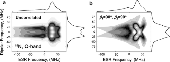

  

  2D DQC (filled) magnitude contour plots computed for ¹⁵N nitroxides using B ₀ = 12500, B ₁ = 60 G, d = 25 MHz with a Gaussian distribution in d (FWHM = 5 MHz). a uncorrelated case; b (β ₁, β ₂) = (90°, 90°), (α ₁, α ₂, γ ₁, γ ₂) = 0. 4 × 10⁴ Monte Carlo trials on a random set in {cosθ, φ, λ ₁, λ ₂, d} were used to generate the data for a; 180 × 180 mesh in {cosθ, φ} and 11 values of d were used to generate b. The 1D dipolar spectra on the right hand sides of a, b are nearly completely smeared and may be suited only to estimate d and its variance. The 2D spectra, however, are quite different. The 2D spectrum in b exhibits a distinct fingerprint of orientational correlation, but the 2D spectrum for the uncorrelated case in a is similar to that in Fig. 5 in that it tends to streak parallel to the ESR frequency axis, as one would expect for such a case, where any point in the ESR spectrum corresponds to all possible orientations

• 5. Figures 7 and 8 illustrate other cases but using two different plotting formats: the former show stack plots and the latter shows contour plots. The 2D simulations were made rigorously for B ₀ = 6200 G, B ₁ = 60 G, d = 25 MHz (12.7 Å). The top two cases represent the situation of pronounced correlations, i.e. (β ₁, β ₂) = (0°, 0°) and (90°, 90°), with the rest of the angles (α ₁, α ₂, γ ₁, γ ₂) being zero. (Note that strong effects of pseudosecular terms are clearly visible over a broad range of distances up to at least 30–35 Å.) The sensitivity to the α _k and γ _k angles mainly depends on their particular combination with the β _k , but in most cases the former angles have much less effect. For example, if for the case of (90°, 90°) one sets α ₂ to 90°, this will bring it close to the (0°, 90°) case (Figs. 7c, 8c), where in a 1D representation it is hard to see a difference from the uncorrelated case (Figs. 7d, 8d). In a 1D plot (especially if distances are distributed) the Pake doublets for the (0°, 90°) case (Figs. 7c, 8c) and uncorrelated case (Figs. 7d, 8d) are hard, if at all possible, to distinguish; but they are quite different in the 2D plots. Note the shapes of the 1D summed spectra. The case in Figs. 7a and 8a [and less so, case in Figs. 7b, 8b] clearly distinguishes itself in the 1D spectrum from the uncorrelated case (Figs. 7d, 8d) and mainly due to the pseudosecular terms. It means that at distances of 35 Å or greater all 1D spectra will be almost identical as in the limiting case of Fig. 5. Even relatively narrow distributions in distance would likely obscure the information on orientations in a 1D plot. The matter about the smearing effect of distance distributions also applies to the cases in Figs. 7a, b and 8a, b, however, in the 2D plot the overall pattern is more immune to this, since for the 2D plot the pattern is distinctly structured and spatially well-resolved. Figure 6 clearly supports this observation.

  Fig. 7

  

  Examples of 2D FT magnitude stack plots for three cases of orientational correlation: a (β ₁, β ₂) = (0°, 0°), b (β ₁, β ₂) = (0°, 90°), c (β ₁, β ₂) = (90°, 90°). The other four angles were set to zero. Case d is the uncorrelated case. Cases a, b correspond to strong correlations, whereas cases c and d are very similar in 1D, but still distinct in 2D plots. In all four cases B ₀ = 6200 G, B ₁ = 60 G, d = 25 MHz

  Fig. 8

  

  The same cases as shown as in Fig. 7, but in a contour plot representation. The magnitude 2D signal was summed along both dimensions and is shown as the 1D ESR absorption spectrum (at the top) or Pake doublets (on the right-hand side)

• 6. An extensive example compiled of 18 plots in Fig. 9a–c is intended to test the accuracy and applicability of efficient ways of signal computation based on analytical approximations for 1D DQC spectra (cf. Appendix 3). The simulations were made for three orientations in angles beta, as indicated. All simulations were made for B ₀ = 6200 G. In Fig. 9, rows a1–a3 show rigorous simulations, while rows b1–b3 are computed using expressions from Ref. [2] [cf. Eqs. 16–18 in Appendix 3]. In Fig. 9a, b rows a1 and b1 correspond to B ₁ = 30 G, d = 52 MHz, which corresponds to 10 Å; rows a2 and b2 are for B ₁ = 60 G, and the same d = 52 MHz. Figure 9c shows the case of B ₁ = 60 G and d = 25 MHz (12.7 Å). In the comparison of a1 with b1 one can clearly see some deviations, especially for (90°, 90°), but they are smaller in the remaining cases. In rows a2 and b2 the differences are still visible but are small enough as to have little practical significance. Finally, for the last case (shown in Fig. 9c) results are virtually indistinguishable. From these results, we can set a “border region” criterion as B ₁ ≲ 2D (or B ₁ ≲ 3d) for which rigorous 1D simulations should be seriously considered.

  Fig. 9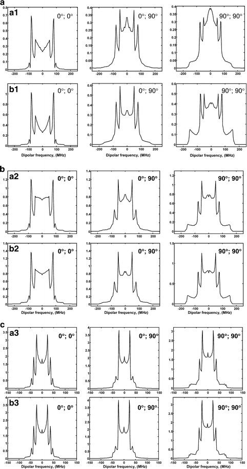

  

  a The comparison of rigorous (a1) and approximate (b1) 1D computations. Three selected cases of nitroxide orientations of beta angles (0°, 0°), (0°, 90°), (90°, 90°) were used. Simulations were made for B ₀ = 6200 G, B ₁ = 30 G, d = 52 MHz. b The comparison of rigorous (a2) and approximate (b2) 1D computations. Three selected cases of nitroxide orientations of beta angles (0°, 0°), (0°, 90°), (90°, 90°) were used. Simulations were made for B ₀ = 6200 G, B ₁ = 60 G, d = 52 MHz. c The comparison of rigorous (a3) and approximate (b3) 1D computations. Three selected cases of nitroxide orientations of beta angles (0°, 0°), (0°, 90°), (90°, 90°) were used. Simulations were made for B ₀ = 6200 G, B ₁ = 60 G, d = 25 MHz

• 7. Figure 10 shows the effect of increasing the amplitude of B ₁ on the maximum of the echo signal expressed by Eq. 11. Looking at the values obtained for B ₁ = 10–100 (and the value at infinity) at d = 25 MHz and B ₀ = 6200 G, one can see from Fig. 10 that it reaches half the value of the basic Hahn echo in an asymptotic manner as B ₁ approaches infinity. This is expected from the basic theory [2]. It should be noted, however, that in the case of large d, when pseudosecular terms are significant, there is a loss of 5–10% of the signal even at infinite B ₁, due to the increase of low-frequency content in the time-domain signal.

  Fig. 10

  

  Normalized echo amplitude as a function of B ₁ and frequency. Plot of the rigorously computed maximum value of the echo signal, Eq. 11, as a function of B ₁ for d = 25 MHz, B ₀ = 6200 G, uncorrelated case (circles) and d = 15 MHz, B ₀ = 34000 G, orientations λ _1,2 = (0°, 0°, 0°) (diamonds). The asymptotic value approaches 0.5 of the basic Hahn echo signal as B ₁ → ∞ (i.e. ideal hard pulses). (But it is 5–10% smaller for large d’s due to the effects of pseudosecular terms producing low-frequency oscillations). Dashed lines Spline interpolations using computed data points. Solid lines Echo maxima as a function of B ₁ computed for uncorrelated orientations of ¹⁴N nitroxides for B ₀ = 6200 G (top solid line) and 34000 G (bottom solid line) from Eq. 18

6 Conclusions and Future Prospects

The main features and conclusions from the simulations presented here are as follows.

• 1. The simulations for cases of short distances (10–15 Å) are rigorously performed using the approaches presented here, where the full spin Hamiltonian is utilized during the pulse. Furthermore, the application of a very strong B ₁ field leads to clean Pake doublets in 1D that enables one to determine the dipolar (and exchange) couplings with the effects of correlations with the nitroxide magnetic tensors largely suppressed, in most cases. Then, in the 2D format one may examine the “fingerprint” and make distinctions amongst different orientations of the principal-axis systems of the magnetic tensors of the nitroxides when correlations are present.

• 2. It was clearly demonstrated that the concept of increased correlation sensitivity in 2D FT spectra is indeed valid.

• 3. We also demonstrate the increased DQC signal strengths obtained by performing experiments with stronger pulses.

• 4. The criterion for using the approximate analytical approach versus rigorous 1D simulations at conventional frequencies (up to Q-band) was established.

• 5. For all practical purposes rigorous DQC simulations should be utilized for the 2D domain, strong coupling cases, and the millimeter-wave range. 1D simulations based on approximate analytic approaches are two to three orders of magnitude computationally more efficient and virtually linearly scalable in multiprocessor-systems. This makes it possible to apply them to more complex 1D cases that include averaging over multiple parameters, data fitting, or to multi-spin systems.

• 6. The pseudosecular terms are useful by providing more telling 1D and 2D dipolar data. The pseudosecular part of the dipolar coupling is responsible for the spectral peaks with 3d/2 splitting when two spins resonate at sufficiently close frequencies. This depends differently on orientational correlations than that for the secular part, leading to a richer 2D spectrum.

• 7. In the presence of distance distributions, the 1D spectrum becomes structureless, however, the 2D spectrum does exhibit patterns that are distinct from those in the absence of correlation.

• 8. With the approach adopted here, the electron spins are treated in the point dipole approximation ignoring spin-density delocalization. For distances less than about 10 Å, one should account for spin-density delocalization, which is significant, e.g. on tyrosyl or flavin radicals, leading to a rhombic dipolar tensor.

• 9. Relaxation effects have not been considered here. Phase relaxation can be introduced phenomenologically as in Refs. [1, 2], but sufficiently fast spin–lattice relaxation does require treatment with full rigor in Liouville space. However, there exist simplified versions that can be used in Hilbert space, see, e.g. Lee et al. [17].

Appendices

Appendix 1: Nitroxide Spin Hamiltonian

The Zeeman and hyperfine part of the nitroxide spin Hamiltonian, H ₀, in the irreducible spherical tensor operator (ISTO) representation takes the form [18–20]:

$$ H_{0} = \sum\limits_{{\mu_{k} ,L,M}} {F_{{\mu_{k} ,\ell }}^{L,M*} A_{{\mu_{k} ,\ell }}^{L,M} } $$

where L is the tensor rank (0 or 2); M = −L, …, L; k = 1, 2 numbers the nitroxides; and ${\ell }$ denotes the reference frame where the tensors are defined, i.e. magnetic frame (g _k ), molecular (dipolar) frame (d), or laboratory frame (l). $A_{{\mu_{k} ,\ell }}^{L,M}$ are the spin operators with μ _k referring to the kind of magnetic interaction, electron Zeeman (g), nuclear Zeeman (N), or hyperfine (A), and they are usually defined in the laboratory frame; $F_{{\mu_{j} ,\ell }}^{L,M}$ is proportional to the ISTO of the magnetic interaction and is most conveniently defined in the g-frame. The transformation of $F_{{\mu_{k} ,g_{k} }}^{L,M}$ to the laboratory frame yields the H ₀. In the high-field limit, where the non-secular terms ($S_{ \pm } ,S_{ \pm } I_{z} ,S_{ \pm } I_{ \pm } ,S_{ \pm } I_{ \mp }$) can be omitted, the ISTO form of the g-tensor reduces to:

$$ \begin{aligned} F_{{g_{k} ,g_{k} }}^{0,0} & = - \sqrt {{\frac{1}{3}}}\,{\frac{{\mu_{B} }}{\hbar }}\left( {g_{xx}^{(k)} + g_{yy}^{(k)} + g_{zz}^{(k)} } \right),\quad A_{{g_{k} ,{l} }}^{0,0} = - \sqrt {{\frac{1}{3}}} B_{0} S_{kz} ; \\ F_{{g_{k} ,g_{k} }}^{2,0} & = - \sqrt {{\frac{2}{3}}}\, {\frac{{\mu_{B} }}{\hbar }}\left[ {g_{zz}^{(k)} - {\frac{1}{2}}\left( {g_{xx}^{(k)} + g_{yy}^{(k)} } \right)} \right],\quad A_{{g_{k} ,{l} }}^{2,0} = - \sqrt {{\frac{2}{3}}} B_{0} S_{kz} ; \\ F_{{g_{k} ,g_{k} }}^{2, \pm 2} & = {\frac{1}{2}}\,{\frac{{\mu_{B} }}{\hbar }}\left( {g_{xx}^{(k)} - g_{yy}^{(k)} } \right),\quad A_{{g_{k} ,{l} }}^{2, \pm 2} = 0. \\ \end{aligned} $$

Similarly, the relevant components of the hyperfine tensor are:

$$ \begin{aligned} F_{{A_{k} ,g_{k} }}^{0,0} & = - \sqrt {{\frac{1}{3}}} \,{\frac{{\mu_{B} }}{\hbar }}\left( {A_{xx}^{(k)} + A_{yy}^{(k)} + A_{zz}^{(k)} } \right),\quad A_{{A_{k} ,{l}}}^{0,0} = - \sqrt {{\frac{1}{3}}} S_{kz}^{{}} I_{kz}^{{}} ; \\ F_{{A_{k} ,g_{k} }}^{2,0} & = - \sqrt {{\frac{2}{3}}} \,{\frac{{\mu_{B} }}{\hbar }}\left[ {A_{zz}^{(k)} - {\frac{1}{2}}\left( {A_{xx}^{(k)} + A_{yy}^{(k)} } \right)} \right],\quad A_{{A_{k} ,{l}}}^{2,0} = - \sqrt {{\frac{2}{3}}} S_{kz} I_{kz} ; \\ F_{{A_{k} ,g_{k} }}^{2, \pm 1} & = 0,\quad A_{{A_{{_{k} }} ,{l}}}^{2, \pm 1} = \mp {\frac{1}{2}}S_{kz} I_{k \pm } ; \\ F_{{A_{k} ,g_{k} }}^{2, \pm 2} & = {\frac{1}{2}}\,{\frac{{\mu_{B} }}{\hbar }}\left( {A_{xx}^{(k)} - A_{yy}^{(k)} } \right),\quad A_{{A_{{_{k} }} ,{l}}}^{2, \pm 2} = 0. \\ \end{aligned} $$

Also, the nuclear Zeeman term (when retained) is given by $\sum\limits_{k} {F_{{N_{k} ,l}}^{0,0} A_{{N_{k} ,l}}^{0,0} }$ with

$$ F_{{N_{k} ,l}}^{0,0} = \sqrt 3 {\frac{{g_{n} \beta_{n} }}{\hbar }},\quad A_{{N_{k} ,l}}^{0,0} = - \sqrt {{\frac{1}{3}}} B_{0} I_{kz} $$

It is noted that the nuclear quadrupole term for ¹⁴N nitroxide is neglected. The second-rank tensors $F_{{\mu ,g_{k} }}^{2,M}$ are transformed in two steps: first, from the kth nitroxide g-tensor axes to the dipolar frame, with its z-axis coincident with the vector r connecting magnetic dipoles, and then to the laboratory frame. The transformations from the dipolar frame to g-frame are defined by the Euler angles $\lambda_{k} \equiv (\alpha {}_{k},\beta_{k} ,\gamma_{k} ) \,$ as shown in Fig. 2 and the transformation from the laboratory frame to the dipolar frame is defined by $\eta \equiv (0,\theta ,\varphi )$. The transformed tensors thus can be written as:

$$ F_{{\mu_{k} ,l}}^{L,M*} = \sum\limits_{{m^{\prime},m^{\prime\prime}}} {D_{{m,m^{\prime}}}^{L} (\eta )} D_{{m^{\prime},m^{\prime\prime}}}^{L} (\lambda_{k} )F_{{\mu_{k} ,g_{k} }}^{L,M} . $$

The Hamiltonian in the laboratory frame takes the form:

$$ H_{0} = \sum\limits_{k} {[S_{kz} (C_{k} + A_{k} I_{kz} + B_{k} I_{k + } + B_{k}^{*} I_{k - } )} + G_{k} I_{kz} ]. $$

The coefficients C _k , A _k , G _k , and B _k are expressed as follows:

$$ C_{k} = \sum\limits_{{m^{\prime}}} {D_{{0,m^{\prime}}}^{2} (\eta_{k}^{{}} )} K_{{g_{k} ,m^{\prime}}} (\lambda_{k} ),\quad A_{k} = \sum\limits_{{m^{\prime}}} {D_{{0,m^{\prime}}}^{2} (\eta_{k}^{{}} )} K_{{A_{k} ,m^{\prime}}} (\lambda_{k} ); $$

$$ 2B_{k} = \sum\limits_{{m^{\prime}}} {D_{{1,m^{\prime}}}^{2} (\eta_{k}^{{}} )} K_{{A_{k} ,m^{\prime}}} (\lambda {}_{k}),\quad G_{k} = \gamma_{nk} B_{0} , $$

where

$$ K_{{\mu_{k} ,m^{\prime}}} (\lambda_{k} ) = [D_{{m^{\prime},2}}^{2} (\lambda_{k}^{{}} ) + D_{{m^{\prime}, - 2}}^{2} (\lambda_{k} )]F_{{\mu_{k} ,g_{k}}}^{2,2} + D_{{m^{\prime},0}}^{2} (\lambda_{k} )F ^{2,0}_{{\mu_{k} ,g_{k}}} $$

includes the transformations $D_{{m^{\prime},m^{\prime\prime}}}^{2} \left( {\lambda_{k} } \right)$ from the dipolar frame to the kth magnetic frame. Since all the transformations were carried out numerically, the explicit expressions for C _k , A _k , and B _k were unnecessary. They are somewhat lengthy and the reader is referred to Saxena and Freed [1]. We just mention that the terms C _k , A _k , and B _k contain all anisotropies in the g and hyperfine tensors as well as the Euler angles needed for their transformation from the respective principal-axes system to the laboratory frame. It is also noted that C _k , G _k , and A _k are real, whereas B _k is complex. Finally, it is noted that in carrying out the computations for B ₀ well up to Q-band (35 GHz), the nuclear Zeeman term can be safely omitted and the H ₀ in real form can be obtained to a high accuracy based on the useful approximation described in Ref. [21].

Appendix 2: Algorithm to Calculate Six-Pulse DQC Echo Signal

This appendix contains the details of how to calculate the final density matrix, ρ _f , from which the DQC echo signal can be calculated as given by Eqs. 14 and 15 below. Basically, this consists of carrying out a series of transformations of the density matrix by a propagator, pulse or free evolution, and choosing the matrix elements of the density matrix after the application of a pulse on a coherence pathway. Here, the direct-product representation for $S_{1} \otimes S_{2} \otimes I_{1} \otimes I_{2}$ to write the matrix elements of the various operators involved in the calculation will be used. To this end, the following details are required.

2.1 Matrix Representation and Notation

For each electron with spin S = 1/2, the matrix dimension is 2, whereas for each nucleus with spin I, it is (2I + 1). Therefore, for the electron–nuclear-spin coupled system of the nitroxide pair the size of the product space is N × N with N = 4(2I ₁ + 1)(2I ₂ + 1), which for ¹⁴N nitroxides is 36 × 36. The Zeeman basis with the basis vectors $\left| k \right\rangle \equiv \left| {m_{1} ,m_{2} ;M_{1} ,M_{2} } \right\rangle$ is used, where $\left| k \right\rangle$s are the eigenvectors of the z-components of the electron and nuclear-spin operators: $S_{z} \left| m \right\rangle = m\left| m \right\rangle^{{}}$ and $I_{z} \left| M \right\rangle = M\left| M \right\rangle$. Here m and M are the electronic and nuclear-spin magnetic quantum numbers, respectively. Lower-case Roman letters will be used to describe the basis state in the product space, Greek letters will be used to describe the eigenvectors of H: $H\left| \alpha \right\rangle = \omega_{\alpha } \left| \alpha \right\rangle$. The Hamiltonian H is diagonalized by the unitary transformation V ^† HV = E, where E is a diagonal matrix of eigenvalues of H and V ^† is Hermitian adjoint of V. The columns of V are the eigenvectors of H: $\left| \alpha \right\rangle_{k} = \left\langle {k} \mathrel{\left | {\vphantom {k \alpha }} \right. \kern-\nulldelimiterspace} {\alpha } \right\rangle \equiv V_{k\alpha }$. In the computations the matrices E and V are the outputs of the matrix diagonalization subroutine, such as JACOBI [22], used here. (A better version of the JACOBI subroutine than that given in [22] can be found on the Netlib website http://netlib.org or is available from the authors.)

2.2 Initial Density Matrix in Product Space

Using the expression for $\rho (0)$ as given by Eq. 2, the initial density matrix is expressed as

$$ {\varvec{\uprho}}_{0} = (S_{1z} \otimes {\mathbf{1}}_{2} + {\mathbf{1}}_{1} \otimes S_{2z} ) \otimes {\mathbf{1}}_{I1} \otimes {\mathbf{1}}_{I2} , $$

(12)

where ${\mathbf{1}}_{{I_{1} }}$ and ${\mathbf{1}}_{{I_{2} }}$ are 3 × 3 unit matrices in the respective nuclear-spin spaces for ¹⁴N nitroxides. A diagonal matrix of order 4 × 4 on the right-hand side of Eq. 12 represents S _z  ≡ S _1z  + S _2z in the product space $S_{1} \otimes S_{2}$ for the two nitroxide electron spins, that is $({\varvec{\upsigma}}_{z} \otimes {\mathbf{1}}_{2} + {\mathbf{1}}_{1} \otimes {\varvec{\upsigma}}_{z} )/2 = {\text{diag(1,0,0,}} - 1 )$, where 1 ₁ and 1 ₂ are 2 × 2 unit matrices in the spin spaces for electrons 1 and 2, respectively.

2.3 Transformation of the Density Matrix by a Propagator

The propagators to be considered here are either a pulse propagator due to a π/2 or a π pulse, or a free-evolution operator in the absence of a pulse. The effects of the various propagators as shown in Fig. 1 are calculated using Eq. 14 below, with the appropriate Hamiltonians and their durations. The procedure for a given density matrix, ρ, and Hamiltonian, H, acting during the time period, t, is described here, which can be specialized for the various propagators by appropriate substitutions, using appropriate times t _k (t _1,2 = t _p ; t _3,4 = t _DQ; t ₅ = t _m  - t _p ; t ₆ = t ₅ + t _echo) and Eqs. 6–10, which describe the Hamiltonians used in the analysis of the six-pulse DQC sequence. The transformed density matrix, ρ′, under the action of a propagator is expressed as:

$$ \rho^{\prime} = {\text{e}}^{ - iHt/\hbar } \rho {\text{e}}^{iHt/\hbar } . $$

(13)

Since ${\text{e}}^{{ - iH_{km} t}} = V_{k\alpha } {\text{e}}^{{ - i\omega_{\alpha } t}} V_{\alpha m}^{*}$ the matrix elements of ρ′ in Eq. 13 can be expressed as $\rho_{jk}^{\prime } = {\text{e}}^{{ - iH_{jm} t}} \rho_{mn} {\text{e}}^{{iH_{nk} t}} = V_{j\alpha } {\text{e}}^{{ - i\omega_{\alpha } t}} V_{m\alpha }^{*} \rho_{mn} V_{n\beta } {\text{e}}^{{ - i\omega_{\beta } t}} V_{k\beta }^{*}$, where summation is conducted over the repeating indexes, or explicitly

$$ \rho_{jk}^{\prime } = \sum\limits_{\alpha ,\beta ,m,n} {\rho_{mn} V_{m\alpha }^{*} V_{n\beta } V_{j\alpha } V_{k\beta }^{*} {\text{e}}^{{ - i\omega_{\alpha \beta } t}} } $$

(14)

with $\omega_{\alpha \beta } \equiv \omega_{\alpha } - \omega_{\beta }$. Equation (14) can be written using a short-hand notation as $\rho^{\prime} = {\mathbf{L}}\rho .$ In this notation L is an operator, which is Q for a free-evolution period or R for the action of a pulse. Coherence pathway selection implies retaining only those elements of ρ′, which belong to the pathways of interest, with the subsequent summation conducted over all pathways that contribute to the echo of interest. In computations this is accomplished by retaining only those matrix elements that correspond to the selected pathway, setting the rest to zero. This may be expressed as the application of a projection operator P (which in reality does not need to be constructed). The final density matrix after application of N pulses and subsequent evolution periods is then calculated as

$$ \rho_{f} (t) = \sum\limits_{{\{ {\mathbf{p}}_{k} \} }} {({\mathbf{Q}}_{N} {\mathbf{P}}_{{{\mathbf{p}}_{N} }} {\mathbf{R}}_{N} , \ldots ,{\mathbf{Q}}_{1} {\mathbf{P}}_{{{\mathbf{p}}_{1} }} {\mathbf{R}}_{1} )\rho (0)} $$

(15)

The product is computed for the full set of coherence pathways {p _k } that contribute to the echo and the sum is then taken to be finally used in computing of $Tr[\rho_{f} S_{ + } ].$

2.4 Coherence Pathway Selection

Subsequent to the action of a pulse propagator of the matrix elements, as calculated in (3) above, all but those in the electronic product subspace of the density matrix ρ that correspond to selected coherence order p should be set to zero. The correspondence of ρ _ik to p is compiled in Table 1 pertinent to the coherence pathways depicted in Fig. 1 illustrating the coherence pathways of the six-pulse DQC sequence. This selection of coherence pathways is achieved experimentally through phase cycling [2] or in computations is based on Table 1.

Table 1 Coherence pathways and respective matrix elements for two coupled spins

Appendix 3: Calculating 1D DQC Signal using Approximate Expressions

Here, we include for completeness the equation from Ref. [2] that was used in this work for making the comparison with 1D DQC signals produced in rigorous computations. The echo amplitude, V, is a function of t _dip = 2t _p  − t _m and is given by

$$ V(t_{\text{dip}} ) = \, K(\omega_{1} )K(\omega_{2} ) \, F(t_{p} )F(t_{m} - t_{p} ). $$

(16)

The time variables are defined in accordance with Fig. 1 and notations in the text. F(t) has the form:

$$ F(t) = (p^{2} + q^{2} \cos Rt)\cos At - q\sin Rt\sin At. $$

(17)

Here A = d(1 − 3cos² θ) and b = −A/2 represent the secular and pseudosecular parts of the dipolar coupling; R ² = Δω ² + b ², where Δω = ω ₁ − ω ₂ is the difference between the Larmor frequencies ω ₁ and ω ₂ of the nitroxide’s electron spins in the frame of reference rotating with the frequency ω _rf of the excitation pulses, which was set to coincide with the center of the nitroxide ESR spectrum. Also, q = b/R and p ² = 1 – q ². The amplitude factors were taken in the simplest possible form as

$$ K(\omega_{k} ) = \left( {{\tfrac{{\omega_{{^{{1{\text{rf}}}} }}^{2} }}{{\Updelta \omega_{k}^{2} + \omega_{{^{{ 1 {\text{rf}}}} }}^{2} }}}\sin^{2} \left( {{\frac{\pi }{2}}\sqrt {1 + \Updelta \omega_{k}^{2} /\omega_{{^{{ 1 {\text{rf}}}} }}^{2} } } \right)} \right)^{3} , $$

(18)

where ω _1rf = γ _e B ₁ for π pulses, which are taken equal here, but do not have to be.

Since ω _k  = ω _k (λ _k ,η), the powder averaging is conducted essentially in the same way as in rigorous computations with ω _k determined for each set of (M ₁, M ₂). This was accomplished using an approximation [21].

References

S. Saxena, J.H. Freed, J. Chem. Phys. 107, 1317–1340 (1997)
P. Borbat, J.H. Freed, in Biological Magnetic Resonance, vol. 19, ed. by L.J. Berliner, S.S. Eaton, G.R. Eaton (Kluwer/Plenum Publications, New York, 2000), pp. 383–459
P.P. Borbat, J.H. Freed, Chem. Phys. Lett. 313, 145–154 (1999)
P.P. Borbat, J.H. Freed, Methods Enzymol. 423, 52–116 (2007)
P.P. Borbat, J.H. Freed, EPR Newsl. 17(2–3), 21–29 (2007)
S. Lee, D.E. Budil, J.H. Freed, J. Chem. Phys. 101, 5529–5558 (1994)
M. Suzuki, J. Math. Phys. 26, 601–612 (1985)
H.F. Trotter, Am. Math. Soc. 10, 545–551 (1959)
R.R. Ernst, G. Bodenhausen, A. Wokaun, Principles of Nuclear Magnetic Resonance in One and Two Dimensions (Clarendon Press, Oxford, 1987)
C. Gemperle, G. Aebli, A. Schweiger, R.R. Ernst, J. Magn. Reson. 88, 241–256 (1990)
S.K. Misra, V. Vasilopoulos, J. Phys. C Condens. Matter 13, 1083–1092 (1983)
T.Y. Li, R.H. Rhee, Numer. Methods 55, 83 (1989)
M. Oettli, Technical Report 205, Department Informatik, ETH, Zurich (1993)
K.E. Gates, M. Griffin, G.R. Hanson, K. Burrage, J. Magn. Reson. 135, 103–112 (1998)
S.K. Misra, J. Magn. Reson. 140, 83–92 (1999)
S.K. Misra, J. Appl. Glob. Res. 2, 38–45 (2009)
S.Y. Lee, B.R. Patyal, J.H. Freed, J. Chem. Phys. 98, 3665–3689 (1993)
J.H. Freed, in Spin Labeling: Theory and Application, chap. 3, ed. by L.J. Berliner (Academic, New York, 1976)
D.J. Schneider, J.H. Freed, in Advances in Chemical Physics, vol. LXXIII, ed. by J.O. Hirschfelder, R.E. Wyatt, R.D. Coalson (Wiley, New York, 1989)
S.K. Misra, J. Magn. Reson. 189, 59–77 (2007)
L.J. Libertini, O.H. Griffith, J. Chem. Phys. 53, 1359–1367 (1970)
W.H. Press, S.A. Teukolsky, W.T. Vetterling, B.P. Flannery, Numerical Recipes in Fortran, 2nd edn. (Cambridge University Press, London, 1992), pp. 456–462
Acknowledgments
The authors are thankful to Ralph “Barry” Robinson for the help with building parallel code and to Dr. Richard H. Crepeau for useful advice. Access to Cornell University Theory Center is greatly acknowledged. This research was supported by NSERC, Canada and NIH/NCRR Grant P41RR016292, USA.
Author information
Authors and Affiliations
Corresponding authors