
Abstract
An extensive uniaxial and triaxial compression testing programme was performed on Indiana Limestone to assess its behaviour across the brittle–ductile transition. Particular attention has been paid to the post-yield evolution of strength and dilatancy. Specimens tested at σ 3 = 30 MPa displayed a fully ductile failure mechanism, whereas specimens tested at σ 3 = 15 MPa and σ 3 = 20 MPa displayed transitional mechanisms, which were neither fully brittle nor fully ductile. Based on an examination of failure localization and dilatancy characteristics, the stress at which crack volumetric strain begins to increase was found to be an indicator of individual specimen ductility. In contrast to less porous rocks, the reversal of total volumetric strain did not coincide with the onset of axial strain nonlinearity under unconfined conditions. With respect to post-yield strength, a major change in the rate of friction mobilization relative to plastic shear strain was observed across the brittle–ductile transition. The dilatancy of the specimens was also found to undergo a major change, with the plastic shear strains to mobilization of peak dilatancy in the ductile regime being approximately one order of magnitude higher than in the brittle regime.
1 Introduction
Knowledge of the complete stress–strain curve for rock materials is necessary to accurately interpret and predict rock deformation behaviour (Wawersik 1975; Singh 1997; ISRM 2007; Arzúa and Alejano 2013). In both the brittle and ductile regimes of deformation, the post-yield behaviour of the rockmass can have implications for both engineered structures in rock such as tunnels and mine workings (i.e. Walton et al. 2014a, 2016; Walton and Diederichs 2015a) or crustal scale geological processes (i.e. Aydin and Johnson 1978; Jamison and Stearns 1982; Simpson 1985; Underhill and Woodcock 1987; Scholz 1988; Boutéca et al. 1996; Fisher et al. 1999; Nagel 2001; Imber et al. 2001; Makowitz and Milliken 2003; Doglioni et al. 2011; Thomas et al. 2012). Several authors have studied the post-yield behaviour of rock, with improvements in testing (Hudson et al. 1971) and measurement (Crouch 1970) techniques enabling the collection of high-quality data (Rummel and Fairhurst 1970; Wawersik and Fairhurst 1970; Wawersik and Brace 1971; Elliott and Brown 1985; Cipullo et al. 1985; Medhurst 1996; Arzúa and Alejano 2013; Walton et al. 2014b).
Although several definitions of the brittle–ductile transition have been proposed, one common definition depends primarily on macroscopic considerations, where the distinction between brittle and ductile behaviour depends on whether or not a macroscopic fracture forms (strain localization occurs) after substantial permanent straining (see Fig. 1) (Paterson and Wong 2005). There are also mechanistic implications for the transition. In carbonate rocks, brittle deformation is cataclastic in nature, where deformation involves microcrack formation and frictional sliding along grain boundaries, whereas ductile deformation (at low temperature) transitions to delocalized cataclasis (or “cataclastic flow”) (Evans et al. 1990; Passchier and Trouw 2005; Paterson and Wong 2005; Wong and Baud 2012). Also, as deformation becomes increasingly ductile, pore collapse begins to play a more significant role than microcracking, leading to an initially compactant stage in porous carbonate rock deformation (although this compactant behaviour ultimately transitions to dilatant behaviour at very large strains) (Wong and Baud 2012).

Schematic illustrating changes in failure patterns in relation to confining stress and ductility
Studies on the brittle–ductile transition in carbonate rocks have typically focused on the nature of the transition itself, including the associated deformation mechanisms (i.e. Mogi 1966; Vajdova et al. 2004, 2012; Wong and Baud 2012) or specifically on post-yield behaviour for a limited range of confining stresses (i.e. Walton et al. 2014b). In this study, post-yield behaviour is considered for a large number of tests performed on Indiana Limestone at a wide variety of confining stresses. The results are considered in the context of brittle theories of deformation (i.e. Martin 1997; Hajiabdolmajid et al. 2002; Diederichs 2003; Walton and Diederichs 2015b) to establish the limits to their application.
2 Testing Methodology
Testing was performed using an MTS Rock Mechanics Testing System, Model 815 (see Fig. 2), at the CANMET Rock Mechanics Laboratory of Natural Resources Canada in Ottawa, Canada. The system consists of independent modules for axial loading and triaxial confinement, both of which are servo-controlled. Tests began with a phase of isotropic confinement of the specimen. During this phase, both the axial and confining stresses were increased at an equal rate of 0.1 MPa/s. Once the desired confining stress was reached, the system was switched to an axial-displacement-control mode for stable control of specimen deformation beyond the peak strength.

MTS Rock Mechanics Testing System (Model 815) used to the collect the data for this study
Axial displacements were recorded using linear variable differential transducers (LVDTs), and circumferential deformation was recorded using a chain extensometer. Volumetric strains were calculated from the measured axial and circumferential strains. These sensors have a specified tolerance of ±1.0% and an actual precision on the order of one-tenth this value. The axial and confining stress values are accurate to ±0.05 and ±0.005 MPa, respectively. Further details on the testing system including specifications are provided by Labrie and Conlon (2008).
In addition to 20 uniaxial compression tests, 34 triaxial compression tests were performed at confining stresses of 2, 4, 5, 8, 10, 15, 20, 30, 40, 50, and 60 MPa. All specimens were tested dry, at ambient laboratory moisture and temperature. Only one test was performed at each of the 40, 50, and 60 MPa levels, as failure was very difficult to induce in these specimens (no failure was observed after axial strains of over 3%). In particular, for the specimens confined at 50 and 60 MPa, the LVDTs reached their effective measurement limit of 5 mm (approximately 5% strain) without showing any signs of instability; for both of these high confinement specimens, the specimens were unloaded, the measurement instruments were reset, and then, the specimens were reloaded as per the loading scheme described above. This step was repeated twice (such that the specimens were loaded three separate times), at which point the specimens began to display significant signs of dilatancy. Although the results for the reloading cycles on these particular specimens are presented for completeness, they should be considered with a degree of scepticism due to the potential effects of an unloading–reloading stress path of the behaviour of these specimens.
Table 1 summarizes the number of tests performed at each level of confining stress.
3 Indiana Limestone
Indiana Limestone is a Mississippian age carbonate rock (323–347 Ma) and can be classified as a grainstone, based on Dunham’s classification (Dunham 1962; Hill 2013). A representative grain-scale image from the block of Indiana Limestone tested in this study is shown in Fig. 3. The grain sizes range from approximately to 0.3–0.5 mm. Based on the dry densities of the specimens tested, and their porosities were found to range between 13.7 and 15.6% with an average of 14.8%. This particular set of Indiana Limestone specimens is both weaker and less porous than the Indiana Limestone specimens that have been tested across the brittle–ductile transition by other authors (i.e. Vajdova et al. 2004, 2012).

Grain-scale image of Indiana Limestone from the block of material tested for this study (after Walton et al. 2014b)
Because of its uniform mineralogy and grain structure (which leads to consistent mechanical behaviour), previous studies have examined its characteristics in the brittle regime (Wawersik and Fairhurst 1970; Robinson 1959; Zheng et al. 1989; Walton et al. 2014b), its tensile fracturing behaviour (Hoagland et al. 1973; Peck et al. 1985), its poroelastic properties (Hart and Wang 1995), its fracture toughness (Schmidt and Huddle 1977), and its behaviour under compactant conditions (Vajdova et al. 2004, 2012; Ji et al. 2012). The uniformity of the specimens tested in this study was confirmed by P-wave velocity measurements made (following the ASTM D2845 procedure) longitudinally along each specimen prior to loading: the P-wave velocities only span a range of 0.23 km/s (see Fig. 4). This corresponds to a coefficient of variation of just under 3%. The low variability in these longitudinal measurements is consistent with the overall uniformity of the samples, as evidenced by a coefficient of variation of 7.5% for the recorded uniaxial compressive strength values, which is at the lower bound of what is typically observed for geological materials (Langford and Diederichs 2015).

Distribution of P-wave velocities of uniaxial and triaxial specimens tested for this study
4 Yield, Strength, and Volumetric Change
4.1 Stress–Strain Response
Qualitatively, a great deal about rock mechanical behaviour can be learned from assessing axial stress–axial strain curves and volumetric strain–axial strain curves. In the case of the Indiana Limestone tests performed for this study, the data have been averaged for each confining stress level to present representative curves (see Fig. 5); variability in these curves between individual tests can be seen in the electronic supplementary material which accompanies this paper. Note that in this study, a compression-positive sign convention has been adopted (positive stresses are compressive in nature, and positive strains represent a decrease in length, circumference, volume, etc.).

a Averaged axial stress–axial strain and b volumetric strain–axial strain curves for each of the confinements tested as well as c examples of strain localization observed in specimens tested at varying confining stress level; note that the strain localization in the case of σ 3 = 60 MPa was caused by both unloading and reloading following yield and the extremely large axial strains imposed over the course of testing (>10%)
As can be seen from the averaged curves, the stress–strain profiles are relatively brittle at low confinement, and transition to a shape which is approximately perfectly plastic around 30–40 MPa of confining stress, with strain-hardening behaviour at higher confinement. Similarly, the transition from primarily dilatant volumetric deformation to compactant deformation occurs around 30 MPa. Both of these results are consistent with a brittle–ductile transition boundary of approximately 30 MPa, where σ 1/σ 3 ≈ 5; this is consistent with the findings of Mogi (1966) who, like Turner et al. (1954) and Griggs et al. (1960), found that the brittle–ductile transition occurs at relatively low confining stress for carbonate rocks, even at low temperatures.
σ 3 ≈ 30 MPa also appears to define the brittle–ductile transition in this case based on the macroscopic definitions of brittle and ductile deformation as proposed by Paterson and Wong (2005). The post-failure photographs of specimens tested at various confinements as shown in Fig. 5 show that in the cases where σ 3 ≥ 30 MPa, no discrete macroscopic fracture/shear zone-controlled specimen deformation can be seen; the exception is the case of the specimen tested at σ 3 = 60 MPa, where macroscopic shear only developed after the specimen had been loaded and unloaded twice, and more than 10% axial strain had been incurred by the specimen. The opposite is true for specimens tested at low confining stress, where clear macroscopic strain localization occurs at relatively low strains.
In the case of the specimens tested at σ 3 = 50 MPa and σ 3 = 60 MPa, only the first loading step is shown for comparison with data collected at other confining stresses. The full range of data collected at σ 3 = 50 MPa and σ 3 = 60 MPa is not readily comparable with the rest of the tests, as the process of unloading to a zero-stress state and reloading is likely to have some unknown effects on the specimen behaviour. For illustrative purposes, however, the data from each of the testing steps for the high confinement data have been qualitatively aligned to show the rough progression of specimen deformation to very large strains (see Fig. 6). In both cases, the specimen behaviour remains overall compactant (positive volumetric strain) up to very large axial strains (~7.5%) and then becomes dilatant. Even as the magnitude of the dilatancy grows significantly, the strain hardening of the specimens continues.

Superimposed axial stress–axial strain and volumetric strain–axial strain plots for the two highest confinements; testing continued over three increments, since strain levels exceeded the measurement limits of the LVDTs used to record axial deformation. The different test phases have been qualitatively aligned to show the progression of specimen deformation. Note that the lack of unloading strains from the first phase of testing of the σ 3 = 60 MPa is due to the induced axial strains exceeding the measurement limits of the LVDTs used
4.2 Crack Initiation, Crack Damage, and Volumetric Strain Reversal
In the brittle regime, the concepts of “Crack Initiation” (CI), “Crack Damage” (CD), and “Volumetric Strain Reversal” are important descriptors of the rock failure process (see Diederichs and Martin 2010 for descriptions of these values); Fig. 7 schematically illustrates these thresholds for stress–strain curves obtained under unconfined conditions. Several authors have demonstrated that the stress at which systematic random cracking occurs under axial loading (CI) corresponds to the onset of nonlinearity in the axial stress–lateral strain curve and that the stress at which cracks begin to interact and propagate in an unstable manner (CD) corresponds to the onset of nonlinearity in the axial stress–axial strain curve (Brace et al. 1966; Martin and Chandler 1994; Martin 1997; Lajtai 1998; Diederichs 2003; Diederichs and Martin 2010). Although originally thought to correspond to CD, the stress at which volumetric strain reversal occurs was later shown to only correspond to CD under unconfined conditions; under confined conditions, the volumetric strain reversal point occurs at a higher stress than CD (Martin 1997; Diederichs 2003; Diederichs and Martin 2010). Even so, the point of volumetric strain reversal still represents a useful landmark with respect to the dilatant behaviour of a specimen.

Schematic representation of crack initiation (CI) and crack damage thresholds (CD) in rock (after Hoek and Martin 2014)
As alluded to above, these thresholds have both mechanistic and empirical significance. At higher confining stresses, however, as the mechanism of deformation changes, the mechanistic significance of these thresholds becomes unclear; empirically, however, the nonlinearities of the axial and lateral strains with respect to axial stress still represent potentially useful indicators for transitions in specimen behaviour. The point of lateral strain nonlinearity was identified based on the crack volumetric strain reversal point; crack volumetric strain was calculated by subtracting elastic volumetric strain (calculated based on data-derived Young’s modulus and Poisson’s ratio values for each specimen) from total volumetric strain, leaving only the inelastic or crack-related component of volumetric strain (Martin 1997). The point of axial strain nonlinearity was evaluated by identifying the stress at which the tangent Young’s modulus begins to decrease from its constant elastic value; tangent modulus values were calculated using adjacent data points and smoothed using a moving average window for visualization purposes (Diederichs and Martin 2010; Walton et al. 2014b).
The crack volumetric strain reversal and axial strain nonlinearity stress values are compared to the peak and residual strengths and volumetric strain reversal stresses in Fig. 8 (generalized Hoek–Brown models (Hoek et al. 2002) are fit to all the data sets, except the crack volumetric strain reversal data, which required a modified Boltzmann sigmoid function (Kaiser and Kim 2015) to fit the observed data). Note that in the strain-hardening regime, “peak strength” is used to denote the point at which the axial stress–axial strain curve was qualitatively assessed to transition from being sub-vertical (initial stiff loading) to sub-horizontal (strain hardening); these qualitative estimates are considered to be accurate within ±10 MPa. Also, in the strain-hardening regime, “residual strength” is used to denote the final steady-state stress level; since no steady-state stress could be assessed for the specimens tested at σ 3 = 50 MPa and σ 3 = 60 MPa, no residual strength values were obtained for these tests.

a Peak strength compared to crack initiation and residual strength and the onset of yield and b the stress at volumetric strain reversal. All models shown were fit using the generalized Hoek–Brown criterion (Hoek et al. 2002) with the m, s, and a parameters allowed to vary except the crack volumetric strain reversal model, which is represented by a modified Boltzmann sigmoid function per Kaiser and Kim (2015)
Under unconfined conditions, Fig. 8 shows that volumetric strain reversal consistently occurred after the point of axial strain nonlinearity. The average unconfined volumetric strain reversal stress is 53.5 MPa versus an average axial strain nonlinearity stress of 38.5 MPa. Martin (1997) and Diederichs and Martin (2010) postulated that these two points should be coincident, based primarily on experience in crystalline rocks; these data suggest that their conclusion may not be valid for porous rocks. The lag in volumetric strain reversal can be explained by the lower tendency of porous sedimentary rocks to dilate relative to crystalline rocks (Alejano and Alonso 2005; Walton et al. 2014b).
An examination of the data suggests that the stress level at which crack volumetric strain reversal occurs may also be an indicator of brittleness or ductility. For σ 3 ≤ 10 MPa, the crack volumetric strain reversal values are consistent with what has typically been observed as CI in brittle crystalline rock: relatively low variability, relatively low confinement dependency, and unconfined values on the order of 40% of the unconfined compressive strength (Martin 1997; Diederichs 2003, 2007; Diederichs and Martin 2010). For σ 3 ≥ 30 MPa, however, the crack volumetric strain reversal values begin to approximate the peak strength envelope, which is also roughly coincident with the volumetric strain reversal envelope. At these high confining stresses, crack volumetric strain reversal no longer represents the same mechanistic indicator as it does for specimens which deform through brittle mechanisms. In fact, at these high confining stresses, the crack volumetric strain reversal values no longer correspond to the point of nonlinearity in the axial stress–lateral strain curve; at these confining stresses, nonlinearity of both the axial and lateral strains begins almost immediately following the onset of differential loading once the desired confining stress is reached through an isotropic loading path (see Fig. 9).

Representative stress–strain and volumetric strain curves for specimens tested at a, c 4 MPa and b, d 40 MPa
This interpretation of the crack volumetric strain reversal data is also consistent with the general conclusion that the behaviour of the Indiana Limestone is fully ductile for σ 3 ≥ 30 MPa (i.e. as shown in Fig. 8 through the convergence of the crack volumetric strain reversal and peak strength envelopes). Additionally, the tendency for the crack volumetric strain reversal envelope to change slope and approach the peak strength envelope starting at σ 3 = 15 MPa can be considered as an indication that this confining stress marks the beginning of a gradual brittle–ductile transition.
This transitional behaviour at intermediate confining stress (15, 20 MPa) is also evidenced by the significant variability in the crack volumetric strain reversal stresses associated with these tests (see Fig. 8). Some of these specimens behave in a relatively ductile manner (higher crack volumetric strain reversal values, closer to the volumetric strain reversal point), whereas others behave in a relatively brittle manner (lower crack volumetric strain reversal values, closer to the expected brittle “Crack Initiation” threshold). Although this difference does not affect the axial stress–axial strain behaviour of the specimen, it does affect the relative dilatant/compactant tendency of the specimen, as well as the degree of strain localization in the specimen and the primary shear band angle of inclination (see Fig. 10). Although some strain localization is shown in all three cases, the degree to which the strain is concentrated within a single shear zone decreases as the crack volumetric strain reversal stress increases; in the more ductile specimens, the strain localization is more diffuse and distributed across a larger number of shear bands.

a Axial stress–axial strain and b volumetric strain–axial strain (bottom) curves for specimens tested at σ 3 = 15 MPa. Also shown are c post-failure photographs of the specimens tested at σ 3 = 15 MPa; dashed lines mark areas of notable shear
The variability observed in these tests indicates that for these transitional confining stress levels, specimens can behave in either a brittle or ductile manner, depending on slight difference between each test. Since the large variability in the behaviour of individual specimens could not be explained by significant grain-scale heterogeneity, other potential causes were examined. It was determined that a slight difference existed between the stress paths of the tests shown in Fig. 10. Although all three tests followed the standard procedure of isotropic loading up to the desired confining stress followed by an increase in only the axial stress, there were slight differences in how long the peak isotropic pressure was maintained prior to increasing the differential stress. In particular, at σ 3 = 15 MPa, the peak uniform isotropic was held for ~1, ~10, and ~40 s for the cases with the highest, middle, and lowest crack volumetric strain reversal stresses. Based on this, it appears that the observed discrepancies in dilatant behaviour (and correspondingly ductility) are consistent with different amounts of viscoelastic (or perhaps viscoplastic) compression which occurred during this time. In the case of the specimen with the lowest crack volumetric strain reversal point, approximately 0.07 mstrain of creep volumetric strain occurred during the ~40 s of constant loading (see Fig. 10, inset). It is possible that this additional amount of compression under isotropic loading led to a grain structure with lower porosity at the onset of differential loading, producing significant dilatancy and strain localization during yield relative to the other specimens tested at the same confining stress. This idea is consistent with the empirical observation that materials with a lower initial porosity tend to dilate more (Walton and Diederichs 2015b).
Ultimately, it is the specimens with higher crack volumetric strain that more closely match the typical testing procedure with minimal delay between isotropic and differential loading. This further suggests that a transition to increasingly ductile behaviour is taking place at σ 3 = 15 MPa and σ 3 = 20 MPa, even if the behaviour cannot be classified as fully ductile based on macroscopic considerations. Interestingly, the transition in the model for crack volumetric strain shown in Fig. 8 approximately corresponds to the line with zero intercept and σ 1/σ 3 ≈ 5 (suggested as the approximately brittle–ductile transition boundary for carbonate rocks by Mogi 1966). All of these results suggest that the crack volumetric strain may serve as a reasonable indicator of the brittle–ductile transition, at least for porous carbonate rocks.
Representative crack volumetric strain profiles (as a function of axial strain) are shown in Fig. 11. Since these profiles are effectively showing how the specimen volumetric strain deviates from an elastic model for volumetric strain, they can be used to draw conclusions about the mechanisms of deformation occurring during specimen loading and to summarize the relationships between ductility, confining stress, crack volumetric strain, and dilatancy. In the case of the unconfined specimen which deforms through brittle mechanisms, the crack volumetric strain profile shows the initial closure of pre-existing cracks followed by the opening and growth of new cracks. In the case of the specimen shown for σ 3 = 20 MPa, which is transitional between the brittle and ductile regimes, fully elastic compression is observed, followed by some very minor inelastic compression, and ultimately, dilatancy. The specimen shown for σ 3 = 40 MPa which deforms through fully ductile mechanisms shows a significant amount of inelastic compression up to large values of axial strain before, ultimately, dilatancy occurs.

Examples of crack volumetric strain plots for specimens tested at confining pressures of a 0 MPa, b 20 MPa, and c 40 MPa. Crack volumetric strain values have been adjusted to show the peak value as “0” for clarity
4.3 Progressive Strength Evolution
The differences in the stress–strain curves shown in Fig. 5 clearly illustrate that strength evolution is a progressive process which occurs over the course of specimen deformation. Through research on brittle deformation mechanisms, several authors have demonstrated that many rocks follow a cohesion-weakening-friction-strengthening (CWFS) strength model (Martin 1997; Hajiabdolmajid et al. 2002; Diederichs 2003, 2007; Walton et al. 2014a, b). In contrast to conventional strength models, the CWFS model is consistent with theoretical and empirical evidence suggesting that the cohesion and friction components of rock strength do not act simultaneously; rather, frictional strength is mobilized over the course of a progressive damage process (often tracked with respect to an inelastic strain quantity) that reduces cohesion from its peak value to a residual value (see Fig. 12).

Schematic illustrating the cohesion-weakening-friction-strengthening (CWFS) strength model, with a loss of cohesion and gain of frictional strength occurring as inelastic strain accumulates within a material (after Walton and Diederichs 2015a)
The procedure for calculating CWFS model parameters from the laboratory data is graphically represented in Fig. 13. First the plastic shear strain γ p at each data point is calculated as the difference between the major and minor principal plastic strains: γ p = \(\varepsilon_{1}^{\text{p}} - \varepsilon_{3}^{\text{p}}\). This plastic shear strain represents a cumulative damage variable to track the deformation process during the course of testing (Alejano and Alonso 2005; Walton et al. 2014b); note that here, yield is defined as the point of axial strain nonlinearity, or equivalently, CD (Zhao and Cai 2010; Chandler 2013; Walton et al. 2014b). For each test, the post-yield stress values from each test were interpolated over a regularly spaced vector of plastic shear strain values. Next, for each value of plastic shear strain, the associated principal stress values of each test are extracted (shown for γ p = 17.5 mstrain in Fig. 13), and a least-squares linear model is used to determine the effective cohesion and friction angle values (based on the intercept and slope of the model, respectively). Because the strength envelope is not perfectly linear, the results obtained depend on the range of confining stresses considered in the analysis; as such, the process described above was repeated using all data from tests with σ 3 ≤ 5 MPa (lowest confinement data), σ 3 ≤ 10 MPa (all fully brittle data), and for all σ 3. The results are shown in Fig. 14.

Schematic illustrating the different stages of CWFS parameter determination—1 raw stress–strain data; 2 yield stress plotted as a function of plastic shear strain; 3 linear fitting using different confining stress ranges for a given plastic shear strain (in this case, γ p = 17.5 mstrain); 4 position of individual cohesion and friction angle points along their evolution profiles

CWFS strength profiles for data at a all confining stresses, b confining stresses of 10 MPa or less, and c confining stresses of 5 MPa or less
As shown in Fig. 14, the Indiana Limestone follows a CWFS strength model both at low confining stresses and at high confining stresses. As the maximum confining stress considered in the strength parameter determination increases, the apparent ultimate (or residual) cohesion tends to increase, whereas the apparent ultimate (or residual or mobilized) friction angle tends to decrease. These changes in the ultimate friction angle can be determined for each individual test by using the servo control to reduce the confining stress to zero while keeping the specimen in a continuous failure state and considering the slope of the line which best fits the resulting σ 1 and σ 3 data (Kovari et al. 1983). These results are shown in Fig. 15, with a logarithmic least-squares model indicating the overall trend in residual friction angle as a function of confining stress.

Residual friction angles as evaluated for individual tests based on analysis of the stresses during unloading. The representative model fit shown is a logarithmic function with a vertical and horizontal offset from the origin
Rather than only considering the results shown in Fig. 14 for a specific subset of confining stresses, it is possible to estimate the cohesion and friction angle for all (σ 3, γ p) conditions. As in the case of the development of the CWFS profiles in Fig. 14, this process begins by interpolating post-yield strength values over regularly spaced intervals of plastic shear strain for each test. Next, for confining stresses with multiple tests, the average post-yield strength at each plastic shear strain was calculated. With an average σ 1–γ p profile having been determined for each confining stress level, the yield surface for the rock can be plotted with respect to σ 3 and γ p (see Fig. 16). This representation of the yield surface shows the initial “hardening” behaviour from yield to peak strength which occurs at very low plastic shear strains; this hardening behaviour which is typically observed in uniaxial and triaxial testing is not intrinsic to the rock material, but rather a consequence of the testing conditions (Diederichs 2007; Bewick et al. 2015). At low confinement, the post-peak strength decreases with increasing shear strain, whereas at high confinement, the post-peak strength continues to increase to very large levels of strain.

Yield strength as a function of confining stress and plastic shear strain
At each pair of (σ 3, γ p) co-ordinates, the instantaneous cohesion and friction angle values can be determined based on a local linear fit to the yield surface shown in Fig. 16 as a function of confining stress. The process for this parameter determination is illustrated in Fig. 17. Instantaneous cohesion and friction angle values were determined for each available (σ 3, γ p) pair by obtaining the least-squares linear fit to the post-yield strength data sharing the same γ p and the nearest confining stresses above and below the level of interest. For example, the instantaneous cohesion and friction for (σ 3, γ p) = (10 MPa, 3 mstrain) were determined based on the linear fit to the post-yield strength data in Fig. 16 for (σ 3, γ p) = (8 MPa, 3 mstrain), (σ 3, γ p) = (10 MPa, 3 mstrain), and (σ 3, γ p) = (15 MPa, 3 mstrain) (see Fig. 17). Using this approach for all (σ 3, γ p) conditions tested allowed maps of cohesion and friction to be produced; additionally, these maps can be re-plotted to show these parameters normalized to their maximum values for each confining stress, which gives a better indication of how much strain is required at each confining stress to result in significant cohesion loss or friction mobilization (see Fig. 18).

Schematic illustrating the different stages of cohesion and friction angle determination for (σ 3 = 10 MPa, γ p = 3 mstrain)—1 averaged σ 1–γ p profiles at each confining stress tested; 2 interpolated visualization of yield strength as a function of confining stress and plastic shear strain with data constraints represented as dots; 3 determination of approximate tangent linear fit to the yield surface at the point of interest; 4 location of the resulting cohesion value on a plot of cohesion as a function of confining stress and plastic shear strain

Cohesion and normalized cohesion (a, b) and friction and normalized friction (c, d) as a function of confining stress and plastic shear strain; note that the normalization of both cohesion and friction is relative to the maximum value for a given confining stress, not the full range of confining stresses tested
As shown in Fig. 18, the most significant changes in the instantaneous cohesion and friction angle occur above σ 3 = 20 MPa. Below this threshold, the commonly used approximation in modelling brittle rock deformation that the plastic shear strains at which the ultimate cohesion and friction angle values are reached are confinement independent remains valid (Hajiabdolmajid et al. 2002; Diederichs 2007; Walton et al. 2014a). Above this threshold, however, there are not only significant changes in the ultimate strength parameters values (i.e. Fig. 18a, c), but also in the plastic shear strains required to reach a quasi-stable strength state (i.e. Fig. 18b, d). In particular, the friction angle requires large plastic shear strains to mobilize to its ultimate value at high confining stress as compared to the almost immediate mobilization of friction at low confining stress.
5 Quantifying Dilatancy
The evolution of dilatancy is strongly tied to the evolution of strength in rock. Cook (1970) demonstrated that in rock, the dilatancy observed in compressive testing results was a manifestation of an inherent tendency of rock to volumetrically expand during yield rather than an artefact of testing conditions. Typically in porous carbonate rocks, although dilatancy occurs under low confinement conditions (and at very large strains under high confinement conditions), as the failure mechanism becomes increasingly ductile, the rock’s volumetric behaviour becomes increasingly compactant (Wong and Baud 2012). To quantify this volumetric behaviour, a commonly used parameter is the dilation angle, ψ, which relates the maximum and minimum principal plastic shear increments (\(\dot{\varepsilon }_{1}^{\text{p}}\) and \(\dot{\varepsilon }_{3}^{\text{p}}\), respectively):
Or, alternatively,
Generally speaking, a higher dilation angle corresponds to larger post-yield inelastic volumetric strains for a given amount of driving strain (i.e. major principal plastic strain, \(\varepsilon_{1}^{\text{p}}\)).
Although originally considered to be a constant parameter (Hill 1950; Vermeer and de Borst 1984), the dilation angle of rock has been demonstrated to vary significantly as a function of both confining stress and the damage state of the rock (typically quantified using the plastic shear strain) (Ofoegbu and Curran 1992; Medhurst 1996; Alejano and Alonso 2005; Zhao and Cai 2010; Walton and Diederichs 2015b). Several models have been proposed to quantify the observed variations in the dilation angle. In this study, the model of Walton and Diederichs (2015b) (referred to hereafter as the “W–D” model) will be used to allow for quantitative study of how the dilatant tendencies of Indiana Limestone change as a function of confining stress.
5.1 The Walton and Diederichs (2015b) Dilation Model
The W–D model consists of a piecewise function for the dilation angle with respect to plastic shear strain. The two distinct components of the model represent the pre-mobilization phase, where the dilation angle rises to its peak value, and the post-mobilization phase, where the dilation angle decays towards zero. The pre-mobilization phase is represented by a logarithmic curve with a tangent linear segment to connect this function to the origin; the post-mobilization phase is represented by an exponential decay function (see Fig. 19). The pre-mobilization parameter, α, controls the curvature of the logarithmic function in the pre-mobilization phase of dilatancy, with lower values corresponding to greater curvature. The dilation mobilization parameter, γ m, indicates the plastic shear strain at which the dilation angle reaches its peak value, ψ Peak, and transitions from the pre-mobilization phase to the post-mobilization phase. The dilation decay parameter, γ *, controls the rate of decay of the dilation angle in the post-mobilization phase of dilatancy.

Walton and Diederichs (2015b) found that the primary effect of confining stress is to reduce the value of the peak dilation angle from being equal to the peak friction angle under unconfined conditions to lower values under confined conditions; the extent to which confining stress affects the peak dilation angle is controlled by two model parameters—β′ and β 0. Walton and Diederichs (2015b) also found that the pre-mobilization curvature and post-mobilization decay of the dilation angle showed some slight trends as a function of confining stress for certain rock types, although in some cases it is reasonable to approximate the pre- and post-mobilization dilatancy trends as confinement independent. Figure 19 illustrates the piecewise W–D model as fit to some sample coal data and shows which parameters control which parts of the model. Indicated in this figure are the four parameters required to define the influence of plastic shear strain on the dilation angle. For a detailed description of the model, readers are referred to the study by Walton and Diederichs (2015b) which outlines the development of the model.
5.2 Changes in Dilatancy as a Function of Confining Stress
Based on an examination of data from a number of different rock types, Walton and Diederichs (2015b) illustrated a general concept for how the dilation angle profile (as shown in Fig. 19, for example) changes as a function of confining stress. Under unconfined conditions, the peak dilation angle equals the peak friction angle, and the post-mobilization decay of the dilation angle is minimal. At low confining stress, the peak dilation angle is still relatively high, and the post-mobilization decay of the dilation angle is large. At relatively high confining stress (near the brittle ductile transition), the dilation angle value tends to reach an approximately constant (and small) value once mobilized (Vermeer and de Borst 1984). Unfortunately, this conceptual model was based on data collected using a relatively limited range of confining stresses.
In Fig. 20, this conceptual model is compared against representative data from the tests performed in this study. Overall, the model and data are relatively consistent, with the caveat that the transition towards an approximately constant dilation angle does not occur at σ 3/σ 1_MAX ≈ 1/3.4 (Mogi’s line for non-carbonate rocks), but at the brittle–ductile transition, which is σ 3/σ 1_MAX ≈ 1/5 for the Indiana Limestone tested in this study. Beyond the brittle–ductile transition, significant compactant behaviour can be observed. In the case of the specimen tested at σ 3 = 60 MPa shown in Fig. 20, the dilation angle begins at an approximately constant value of ψ ≈ −25° and then gradually increases to a positive value (dilation, rather than compression) after significant deformation. Although the parameters describing the mobilization of peak dilatancy and post-mobilization dilatancy are still relevant in this case, the pre-mobilization parameter (α) is meaningless when compactant inelastic volumetric behaviour precedes dilatancy, as the W–D model assumes that the pre-mobilization dilation angle starts at a value of ψ = 0° at the onset of yield.

A hypothesized model for dilation angle profile changes as a function of confinement proposed by Walton and Diederichs (2015b) and corresponding dilation angle profiles at a variety of confining stresses with the W–D (Walton and Diederichs 2015b) dilation models fit to the data; note the different scale used for the σ 3 = 60 MPa data
When considering how each of parameters of the W–D model (as illustrated in Fig. 19) changes with confining stress, the following items can be noted:
-
Pre-mobilization parameter (α): this parameter shows an approximately linear trend with confining stress, as found by Walton and Diederichs (2015b). As stated above, the pre-mobilization dilatancy parameter cannot be defined in the ductile regime.
-
Dilation mobilization parameter (γ m): Of all the dilation model parameters considered, this parameter most clearly shows the brittle–ductile transition (see Fig. 21). For tests conducted in the brittle regime (σ 3 ≤ 20 MPa), the mobilization parameter can be considered as roughly constant as per the suggestion of Walton and Diederichs (2015b). In the ductile regime (σ 3 ≥ 30 MPa), the mobilization of peak dilatancy is significantly delayed, however, as the onset of dilatancy is somewhat delayed due to an initial compactant phase.
Fig. 21 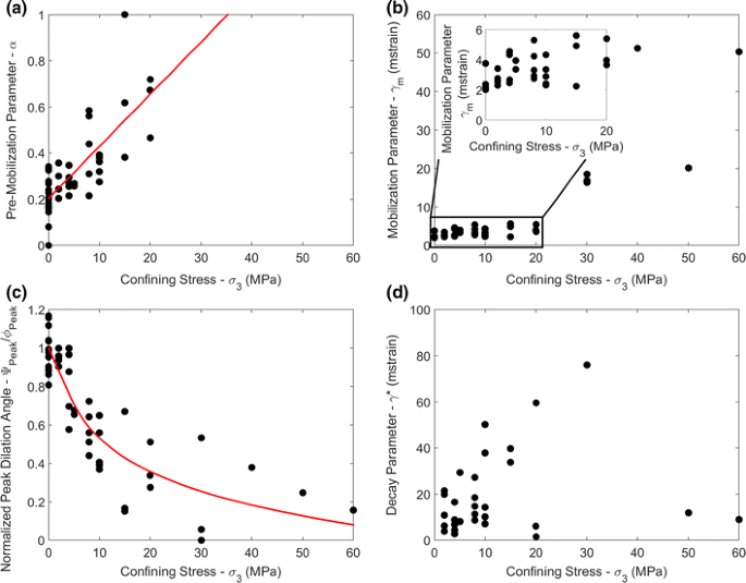
W–D dilation parameters as a function of confining stress—a the pre-mobilization parameter and associated linear fit; b the plastic shear strain at peak dilation angle mobilization; c the normalized peak dilation angle and associated logarithmic fit with a tangent linear transition to (0, 1); d the dilation decay parameter. Linear and logarithmic fits are shown in a and c as per the relationships proposed by Walton and Diederichs (2015b)
-
Peak dilation angle (ψ Peak): these values generally agree with the W–D dilation model, although there appears to be a tendency for peak dilation angles to take on higher values than expected in the ductile regime. It is hypothesized that this can be explained by the very large strains required to mobilize dilatancy in the ductile regime, which are roughly one order of magnitude larger than those in the brittle regime, as well as the significant pre-dilatancy compression which occurs, ultimately leading to need for dilatancy to occur for the specimen to accommodate further straining.
-
Dilation decay parameter (γ *): these values generally show a trend which is consistent with the conceptual model shown in Fig. 20. Under unconfined conditions, almost no post-mobilization decay occurs (in Fig. 21, the unconfined decay parameter values are very large and do not appear within the axis limits of the chart shown). With a slight increase in confinement, there is a rapid decrease in the decay parameter (up to a confining stress of around σ 3 = 4 MPa in the case of this Indiana Limestone). Then as confining stress increases further, the decay parameter values increase approximately linearly as the peak dilation angle decreases and the post-mobilization dilation angle approaches a constant value. At high confining stress in the ductile regime, the decay values drop again, as post-compression dilatancy tends to decay relatively rapidly following mobilization.

In examining the data in Fig. 21, the relatively large dispersion in parameter values at σ 3 = 20 MPa is immediately apparent. Since similar variability was seen in the crack volumetric strain reversal values of these specimens (see Fig. 8), potential relationships between the crack volumetric strain reversal values and the dilation model parameters were investigated. In Fig. 22, these relationships are illustrated, with the stress at crack volumetric strain reversal being strongly related to all four dilation angle model parameters for the σ 3 = 20 MPa data. Since it appears that the crack volumetric strain reversal stress can be taken as a qualitative measure of individual specimen ductility in the brittle–ductile transition, these relationships can be compared against general trends for expected changes in dilatancy with increased ductility. With respect to the relationship between dilatancy parameters and the crack volumetric strain reversal stress, the following conclusions are most readily apparent:
-
Pre-mobilization parameter (α): In the case of this parameter, the trend that the more ductile specimens take on higher values is in agreement with the general trend shown in Fig. 21, where specimens at higher confinements also take on higher values (a least-squares linear model illustrates the trend).
-
Dilation mobilization parameter (γ m): This parameter shows a slight downward trend as a function of crack volumetric strain reversal stress, although the magnitude of this trend is very small relative to the overall variability in this parameter shown in Fig. 21.
-
Peak dilation angle (ψ Peak): This parameter follows a similar trend in Figs. 21 and 22—the more brittle specimens with lower confining stress or lower crack volumetric strain reversal stress tend to have a higher peak dilation angle.
-
Dilation decay parameter (γ *): the most brittle specimen tested at σ 3 = 20 MPa is consistent with the linear trend in this parameter for more brittle samples (lower confinements) shown in Fig. 21. The more ductile specimens, however, show lower values of this parameter which are consistent with the values observed for samples tested at higher confining stresses (50, 60 MPa).
Overall, these results are consistent with the original suggestion that the crack volumetric strain reversal stress is representative of individual specimen ductility and that it influences sample dilatancy accordingly.

Variability in W–D dilation model parameters for specimens tested at σ 3 = 20 MPa as a function of the crack volumetric strain reversal stress. Linear models are fit to all parameters shown except the decay parameter, γ *, which has been fit using an exponential model
6 Conclusions
This study represents an investigation of a large database of compression tests performed on Indiana Limestone over a wide range of confining stresses. Based on visual observation of specimen failure mechanisms as well as an inspection of the averaged axial stress–axial strain curves, the confining stress threshold for fully ductile deformation at ambient room temperature was found to be between σ 3 = 20 MPa and σ 3 = 30 MPa. The crack volumetric strain reversal stress, which is typically considered an indicator of crack initiation in the brittle regime, was found to transition to coincide roughly with the peak stress at high confinement and is suggested to indicate the onset of the brittle–ductile transition when it deviates from the typical CI envelope. The total volumetric strain reversal stress was found to be higher than the onset of axial strain nonlinearity (CD in the brittle regime), which is different from the behaviour observed in low-porosity rocks, where these two parameters are coincident under uniaxial conditions.
In examining the post-yield strength evolution of specimens at different confining stresses, the CWFS strength model was found to be generally appropriate for capturing the observed behaviour. The parameters of this model, however, change significantly as the confining stress exceeds the brittle–ductile transition. In particular, the commonly used approximation in modelling brittle rock deformation that the plastic shear strains at which the ultimate cohesion and friction angle values are reached are confining stress independent is not valid beyond the brittle–ductile transition. The mobilization of the friction angle to its peak value is especially delayed for ductile deformation relative to brittle deformation.
Post-yield dilatancy was also considered in the context of a model which captures the confining stress and plastic shear strain dependencies of the dilation angle. Although the W–D dilation model can be applied to individual tests at all confining stresses, the pre-mobilization portion of the model is inadequate in the ductile regime, as the existence of an initial compactant phase violates the assumption of an initial dilation angle of zero degrees, which is inherent in the model’s formulation. Considering the entire data set, the trends identified as a function of confining stress by Walton and Diederichs (2015b) either become less reliable or wholly invalidated for tests performed in the ductile regime. A close examination of the data revealed that dilation model parameters strongly depend on the crack volumetric strain reversal stress, even when holding confining stress constant; the specimens with higher crack volumetric strain reversal stress values were found to have dilation model parameters similar to those expected at higher confining stress. This finding further suggests that the crack volumetric strain reversal stress can be used as an indicator of brittleness or ductility.
References
Alejano LR, Alonso E (2005) Considerations of the dilatancy angle in rocks and rock masses. Int J Rock Mech Min Sci 42(4):481–507
Arzúa J, Alejano LR (2013) Dilation in granite during servo-controlled triaxial strength tests. Int J Rock Mech Min Sci 61:43–56
Aydin A, Johnson AM (1978) Development of faults as zones of deformation bands and as slip surfaces in sandstone. Pure Appl Geophys 116(4–5):931–942
Bewick RP, Amann F, Kaiser PK, Martin CD (2015) Interpretation of UCS test results for engineering design. In: 13th ISRM international congress of rock mechanics. International Society for Rock Mechanics
Boutéca M, Sarda JP, Schneider F (1996) Subsidence induced by the production of fluids. Oil Gas Sci Technol 51(3):349–379
Brace WF, Paulding BW, Scholz C (1966) Dilatancy in the fracture of crystalline rocks. J Geophys Res 71(16):3939–3953
Chandler NA (2013) Quantifying long-term strength and rock damage properties from plots of shear strain versus volume strain. Int J Rock Mech Min Sci 59:105–110
Cipullo A, White W, Lee IK (1985) Computer controlled volumetric strain measurements in metadolerite. Bull Int Assoc Eng Geol (Bull Assoc Int Géol Ing 32(1):55–65
Cook NGW (1970) An experiment proving that dilatancy is a pervasive volumetric property of brittle rock loaded to failure. Rock Mech 2(4):181–188
Crouch SL (1970) Experimental determination of volumetric strains in failed rock. Int J Rock Mech Min Sci Geomech Abstr 7(6):589–603
Diederichs MS (2003) Manuel Rocha medal recipient: rock fracture and collapse under low confinement conditions. Rock Mech Rock Eng 36(5):339–381
Diederichs MS (2007) The 2003 Canadian Geotechnical Colloquium: mechanistic interpretation and practical application of damage and spalling prediction criteria for deep tunnelling. Can Geotech J 44(9):1082–1116
Diederichs MS, Martin CD (2010) Measurement of spalling parameters from laboratory testing. In: Rock mechanics and environmental engineering. Proceedings of the European rock mechanics symposium, pp 323–326
Doglioni C, Barba S, Carminati E, Riguzzi F (2011) Role of the brittle–ductile transition on fault activation. Phys Earth Planet Inter 184(3):160–171
Dunham RJ (1962) Classification of carbonate rocks according to depositional texture. Am Assoc Pet Geol Mem 1:108–121
Elliott GM, Brown ET (1985) Yield of a soft, high porosity rock. Geotechnique 35(4):413–423
Evans B, Fredrich JT, Wong TF (1990) The brittle–ductile transition in rocks: recent experimental and theoretical progress. Brittle–Ductile Trans Rocks Geophys Monogr Ser 56:1–20
Fisher QJ, Casey M, Clennell MB, Knipe RJ (1999) Mechanical compaction of deeply buried sandstones of the North Sea. Mar Pet Geol 16(7):605–618
Griggs DT, Turner FJ, Heard HC (1960) Deformation of rocks at 500° to 800° C. Geol Soc Am Mem 79:39–104
Hajiabdolmajid V, Kaiser PK, Martin CD (2002) Modelling brittle failure of rock. Int J Rock Mech Min Sci 39(6):731–741
Hart DJ, Wang HF (1995) Laboratory measurements of a complete set of poroelastic moduli for Berea sandstone and Indiana limestone. J Geophys Res Solid Earth (1978–2012) 100(B9):17741–17751
Hill R (1950) The mathematical theory of plasticity. Oxford University Press, London
Hill JR (2013) Indiana limestone. Retrieved 08/01/2013 from http://igs.indiana.edu/MineralResources/Limestone.cfm
Hoagland RG, Hahn GT, Rosenfield AR (1973) Influence of microstructure on fracture propagation in rock. Rock Mechanics 5(2):77–106
Hoek E, Martin CD (2014) Fracture initiation and propagation in intact rock—a review. J Rock Mech Geotech Eng 6(4):287–300
Hoek E, Carranza-Torres C, Corkum B (2002) Hoek–Brown failure criterion-2002 edition. Proc NARMS-TAC 1:267–273
Hudson JA, Brown ET, Fairhurst C (1971) Optimizing the control of rock failure in servo-controlled laboratory tests. Rock Mech 3(4):217–224
Imber J, Holdsworth RE, Butler CA, Strachan RA (2001) A reappraisal of the Sibson-Scholz fault zone model: the nature of the frictional to viscous (“ brittle–ductile”) transition along a long-lived, crustal-scale fault, Outer Hebrides, Scotland. Tectonics 20(5):601–624
ISRM (2007) The complete ISRM suggested methods for rock characterization, testing and monitoring: 1974–2006. In: Ulusay R, Hudson JA (eds) Prepared by the commission on testing methods. ISRM, Ankara
Jamison WR, Stearns DW (1982) Tectonic deformation of Wingate Sandstone, Colorado National Monument. AAPG Bull 66(12):2584–2608
Ji Y, Baud P, Vajdova V, Wong TF (2012) Characterization of pore geometry of Indiana limestone in relation to mechanical compaction. Oil Gas Sci Technol (Rev IFP Energ Nouv 67(5):753–775
Kaiser PK, Kim BH (2015) Characterization of strength of intact brittle rock considering confinement-dependent failure processes. Rock Mech Rock Eng 48(1):107–119
Kovari K, Tisa A, Attinger RO (1983) The concept of “continuous failure state” triaxial tests. Rock Mech Rock Eng 16(2):117–131
Labrie D, Conlon B (2008) Hydraulic and poroelastic properties of porous rocks and concrete materials. In: Proceedings of the 42nd US rock mechanics symposium (USRMS). American Rock Mechanics Association, Paper 08-182
Lajtai EZ (1998) Microscopic fracture processes in a granite. Rock Mech Rock Eng 31(4):237–250
Langford JC, Diederichs MS (2015) Quantifying uncertainty in Hoek–Brown intact strength envelopes. Int J Rock Mech Min Sci 74:91–102
Makowitz A, Milliken KL (2003) Quantification of brittle deformation in burial compaction, Frio and Mount Simon Formation sandstones. J Sediment Res 73(6):1007–1021
Martin CD (1997) Seventeenth Canadian geotechnical colloquium: the effect of cohesion loss and stress path on brittle rock strength. Can Geotech J 34(5):698–725
Martin CD, Chandler NA (1994) The progressive fracture of Lac du Bonnet granite. Int J Rock Mech Min Sci Geomech Abstr 31(6):643–659
Medhurst TP (1996) Estimation of the in situ strength and deformability of coal for engineering design. PhD thesis, University of Queensland, Australia
Mogi K (1966) Pressure dependence of rock strength and transition from brittle fracture to ductile flow. Bull Earthq Res Inst Tokyo Univ 44:215–232
Nagel NB (2001) Compaction and subsidence issues within the petroleum industry: from Wilmington to Ekofisk and beyond. Phys Chem Earth Part A 26(1):3–14
Ofoegbu GI, Curran JH (1992) Deformability of intact rock. Int J Rock Mech Min Sci Geomech Abstr 29(1):35–48
Passchier CW, Trouw RA (2005) Microtectonics, 2nd edn. Springer, Berlin
Paterson MS, Wong TF (2005) Experimental rock deformation-the brittle field. Springer, Berlin
Peck L, Barton CC, Gordon RB (1985) Microstructure and the resistance of rock to tensile fracture. J Geophys Res Solid Earth (1978–2012) 90(B13):11533–11546
Robinson LH (1959) The effect of pore and confining pressure on the failure process in sedimentary rock. In: Proceedings of the 3rd US symposium on rock mechanics (USRMS). American Rock Mechanics Association
Rummel F, Fairhurst C (1970) Determination of the post-failure behavior of brittle rock using a servo-controlled testing machine. Rock Mech 2(4):189–204
Schmidt RA, Huddle CW (1977) Effect of confining pressure on fracture toughness of Indiana limestone. Int J Rock Mech Min Sci Geomech Abstr 14(5):289–293
Scholz CH (1988) The brittle-plastic transition and the depth of seismic faulting. Geol Rundsch 77(1):319–328
Simpson C (1985) Deformation of granitic rocks across the brittle–ductile transition. J Struct Geol 7(5):503–511
Singh AB (1997) Study of rock fracture by permeability method. J Geotechn Geoenviron Eng 123(7):601–608
Thomas AM, Bürgmann R, Shelly DR, Beeler NM, Rudolph ML (2012) Tidal triggering of low frequency earthquakes near Parkfield, California: implications for fault mechanics within the brittle‐ductile transition. J Geophys Res Solid Earth (1978–2012) 117(B5)
Turner FJ, Griggs DT, Heard H (1954) Experimental deformation of calcite crystals. Geol Soc Am Bull 65(9):883–934
Underhill JR, Woodcock NH (1987) Faulting mechanisms in high-porosity sandstones; new red sandstone, Arran, Scotland. Geol Soc Lond Spec Publ 29(1):91–105
Vajdova V, Baud P, Wong TF (2004) Compaction, dilatancy, and failure in porous carbonate rocks. J Geophys Res Solid Earth (1978–2012) 109(B5)
Vajdova V, Baud P, Wu L, Wong TF (2012) Micromechanics of inelastic compaction in two allochemical limestones. J Struct Geol 43:100–117
Vermeer PA, De Borst R (1984) Non-associated plasticity for soils, concrete and rock. HERON 29(3):1984
Walton G, Diederichs MS (2015a) A mine shaft case study on the accurate prediction of yield and displacements in stressed ground using lab-derived material properties. Tunn Undergr Space Technol 49:98–113
Walton G, Diederichs MS (2015b) A new model for the dilation of brittle rocks based on laboratory compression test data with separate treatment of dilatancy mobilization and decay. Geotech Geol Eng 33(3):661–679
Walton G, Arzua J, Alejano LR, Diederichs MS (2014a) A laboratory-testing-based study on the strength, deformability, and dilatancy of carbonate rocks at low confinement. Rock Mech Rock Eng 48(3):941–958
Walton G, Diederichs MS, Alejano LR, Arzúa J (2014b) Verification of a laboratory-based dilation model for in situ conditions using continuum models. J Rock Mech Geotech Eng 6(6):522–534
Walton G, Diederichs M, Punkkinen A, Whitmore J (2016) Back analysis of a pillar monitoring experiment at 2.4 km depth in the Sudbury Basin, Canada. Int J Rock Mech Min Sci 85(1):33–51
Wawersik WR (1975) Technique and apparatus for strain measurements on rock in constant confining pressure experiments. Rock Mech 7(4):231–241
Wawersik WR, Brace WF (1971) Post-failure behavior of a granite and diabase. Rock Mech 3(2):61–85
Wawersik WR, Fairhurst C (1970) A study of brittle rock fracture in laboratory compression experiments. Int J of Rock Mech Min Sci Geomech Abstr 7(5):561–575
Wong TF, Baud P (2012) The brittle–ductile transition in porous rock: a review. J Struct Geol 44:25–53
Zhao XG, Cai M (2010) A mobilized dilation angle model for rocks. Int J Rock Mech Min Sci 47(3):368–384
Zheng Z, Cook NG, Myer LR (1989) Stress induced microcrack geometry at failure in unconfined and confined axial compressive tests. In: Proceedings of the 30th US symposium on rock mechanics (USRMS). American Rock Mechanics Association
Acknowledgements
The authors would like to acknowledge the help of Sean Cowie in developing the brittle damage schematic used in this paper.
Author information
Authors and Affiliations
Corresponding author
Electronic supplementary material
Below is the link to the electronic supplementary material.
Rights and permissions
About this article

Cite this article
Walton, G., Hedayat, A., Kim, E. et al. Post-yield Strength and Dilatancy Evolution Across the Brittle–Ductile Transition in Indiana Limestone. Rock Mech Rock Eng 50, 1691–1710 (2017). https://doi.org/10.1007/s00603-017-1195-1
Received:
Accepted:
Published:
Issue Date:
DOI: https://doi.org/10.1007/s00603-017-1195-1