
Abstract
Most of the railway tunnels in Sweden are shallow-seated (<20 m of rock cover) and are located in hard brittle rock masses. The majority of these tunnels are excavated by drilling and blasting, which, consequently, result in the development of a blast-induced damaged zone around the tunnel boundary. Theoretically, the presence of this zone, with its reduced strength and stiffness, will affect the overall performance of the tunnel, as well as its construction and maintenance. The Swedish Railroad Administration, therefore, uses a set of guidelines based on peak particle velocity models and perimeter blasting to regulate the extent of damage due to blasting. However, the real effects of the damage caused by blasting around a shallow tunnel and their criticality to the overall performance of the tunnel are yet to be quantified and, therefore, remain the subject of research and investigation. This paper presents a numerical parametric study of blast-induced damage in rock. By varying the strength and stiffness of the blast-induced damaged zone and other relevant parameters, the near-field rock mass response was evaluated in terms of the effects on induced boundary stresses and ground deformation. The continuum method of numerical analysis was used. The input parameters, particularly those relating to strength and stiffness, were estimated using a systematic approach related to the fact that, at shallow depths, the stress and geologic conditions may be highly anisotropic. Due to the lack of data on the post-failure characteristics of the rock mass, the traditional Mohr–Coulomb yield criterion was assumed and used. The results clearly indicate that, as expected, the presence of the blast-induced damage zone does affect the behaviour of the boundary stresses and ground deformation. Potential failure types occurring around the tunnel boundary and their mechanisms have also been identified.
1 Introduction
Due to the increasing demand for space, it is nowadays very common to see traffic in populated areas being diverted underground. This requires the excavation of rocks of various natures and characteristics. In Sweden, this is mostly done in brittle rock with intact compressive strength often exceeding 200 MPa. Since drilling and blasting is commonly used in such hard rock masses, it leaves behind a zone of damaged rock immediately around the tunnel boundary, which is referred to as the blast-induced damaged zone or BIDZ, as denoted in this paper. Generally, this zone is characterised by the reduction in its strength and stiffness and the perceived implications are clear, in that they relate mainly to construction and maintenance costs, safety and the long-term performance of the tunnel.
The consequences of blast damage to the rock around a tunnel have been, for a long time, assessed in terms of overbreak rather than accounting for the actual features of damage (e.g. Raina et al. 2000). Forsyth and Moss (1991) define overbreak as the breakage or reduction in the rock mass quality beyond the design perimeter of the excavation. Incidentally, many of the empirical methods for assessing blast damage, including the peak particle velocity (PPV) method by Holmberg and Persson (1980), are related to assessing the overbreak. Saiang (2004) pointed out that much of the effort in blast damage quantification has been largely focussed on defining the depth or extent of the damage, and less on assessing its inherent properties, such as its strength and stiffness. Although the strength and stiffness are the most difficult parameters to measure, they are also the most relevant and reliable parameters for assessing the competency of the rock and, thus, the stability and performance of a tunnel.
Many authors, for example, Oriad (1982), MacKown (1986), Ricketts (1988), Plis et al. (1991), Forsyth and Moss (1991), Persson et al. (1996) and Raina et al. (2000) have deliberated on the importance of blast damage assessment. The Swedish Rock Engineering Research group (SveBeFo) performed an extensive investigation into blast-induced damaged rock in hard rocks over a 4-year period from 1993 to 1996 (Olsson and Bergqvist 1993; Olsson and Bergqvist 1995; Fjellborg and Olsson 1996; Ouchterlony 1997; Olsson and Bergqvist 1997 and Olsson and Ouchterlony 2003). One of the results of this investigation was the development of guidelines that correlate blast-induced damage zone depth to explosive charge concentration (e.g. Ouchterlony et al. 2001). Investigations into the blast-induced damage around tunnels have also been performed elsewhere, for example, Pusch and Stanfors (1992), Hustrulid (1994), da Gama (1998), Nyberg and Fjellborg (2002) and Malmgren et al. (2007). The radioactive waste isolation groups, such as SKB in Sweden and URL in Canada, have also investigated and modelled the BIDZ in hard rock masses (e.g. Martino and Martin 1996; Martino 2003). Holmberg (1982) outlined the important factors that influence the development and extent of blast damage.
One of the important reasons for assessing blast-induced damaged rock around tunnels is stability. In this respect, the strength and stiffness of this zone are the most important parameters. Up until now, the quantification of these parameters has been difficult. Hence, incorporating this zone in the early design stage of a tunnel, which usually involves computer models, is not easy and, therefore, often either neglected or, if attempted, it is modelled using procedures intended for undamaged rock masses. Numerical modelling of the damaged rock mass around a tunnel has been done using both continuum and discontinuum methods. However, Barla et al. (1999) noted that the key to the success of any numerical modelling process is the level of understanding achieved in describing the rock mass conditions. This can be made more difficult if the blast-induced damaged zone requires consideration in the analysis, especially that a quantitative understanding of the mechanical characteristics of this zone will be required. Without this quantitative understanding, the continuum method of analysis usually takes precedence over the discontinuum method, because the latter requires an explicit description of the rock mass. Hence, many investigators, among others, Yang et al. (1993), Feng et al. (2000), Sheng et al. (2002) and Sato et al. (2000), have used the continuum method to study the behaviour of the damaged rock mass close to an excavation boundary.
This paper presents an elasto-plastic numerical study of the mechanical behaviour of the blast-induced damaged rock around shallow-seated tunnels in brittle rock mass. The continuum method of numerical analysis was assumed and the finite-difference code FLAC (Itasca 2002) was utilised. The input parameters for the rock mass and in-situ stresses are those typically encountered in shallow tunnel projects in Sweden. The tunnel profiles used are those typically used by Swedish Railroad Administration. The extent of the blast-induced damage is decided beforehand and is based on the works of the Swedish Rock Engineering Research and Swedish Railroad Administration guidelines. The study is principally presented in the form of a parameter study to observe the effects of the BIDZ on the overall response of the near-field host rock. The effects on the boundary stress and ground deformation characteristics due to variation in the inherent properties of the damaged rock, namely, strength and stiffness, and other related parameters were studied. The development of the models involved using typical scenarios encountered in railway tunnelling projects in Sweden. For the values of the input parameters, the common practice approach was used, but more systematically so in order to obtain input values for the BIDZ.
2 Background
2.1 Purpose of the Study and Approach
An important question is whether the presence of the blast-induced damaged rock around a shallow tunnel is important or not for stability and performance. By intuition and also considering the nature of the excavation, it is usually considered to be important and is, thus, a factor in design and construction guidelines. However, this consideration is largely based on methods related to overbreak, as noted elsewhere. These methods do not measure the competency of the damaged rock. It is the inherent properties of damaged rock, particularly its strength and stiffness, which provide a measure of the competency and, thus, relate directly to the stability and performance of the tunnel. Admittedly, these parameters are very difficult to measure in practice. However, numerical methods can be used to test different scenarios when the inherent characteristics of the BIDZ are varied. This paper, therefore, progresses in that direction.
Numerical modelling of the BIDZ has also been difficult, mainly because of the lack of quantitative understanding of the inherent characteristics of the blast-induced damaged rock. Attempts to model this zone in practical design cases are mainly based on procedures intended for undamaged or undisturbed rock masses and simple constitutive models, while also ignoring anisotropy.
This numerical study aims to investigate the influence of the blast-induced damaged rock on the overall response of the near-field host rock when various parameters, either inherent to the damaged rock or external, such as in-situ stresses, are varied. In doing so, the important parameters of the blast-induced damaged rock, as well as those which can directly influence the response of the BIDZ, can be identified. Because of the complexity of the BIDZ, the modelling approach used follows commonly employed approaches, in particular, those that would be generally applied by consultants and design engineers. One of the objectives, therefore, is to demonstrate whether these commonly used practices are adequate for modelling blast-induced damaged rock or not.
2.2 Physical and Mechanical Characteristics of Blast-Induced Damaged Rock
Figure 1 shows a saw-cut through a granite block showing the characteristic fracture patterns after perimeter blasting. If these patterns are superimposed onto a tunnel boundary, the result will be as shown in Fig. 2. Such a complex physical state of the BIDZ rock can significantly influence the mechanical response of the damaged rock mass and, consequently, the overall rock mass around the fractured zone. The failure mechanisms will also be affected. Theoretically, the mechanical characteristics of the near-field host rock, in terms of important mechanical and hydraulic parameters, are as shown in Fig. 3.

Characteristic fracture pattern around Ø64-mm blastholes in granitic rock (from Olsson and Bergqvist 1995). The explosive type used was Kumulux 22. The factures are of different lengths, shapes and sizes, and the estimated thickness of the damage zone was 25 cm

Rock mass condition around a tunnel boundary excavated by drilling and blasting. The damaged zone comprises discontinuous fractures of microscopic to macroscopic sizes, with complex fracture patterns due to radial cracks (see embedded figure, adopted from Whittaker et al. 1992) from adjacent blastholes

A conceptual model of the excavation disturbed zone and its characteristics in terms of the quantities generally investigated: a is the zone of intense fracturing, generally referred to as the damaged zone, and b is the disturbed zone, where disturbance is largely due to stress re-distribution, resulting in the opening and closing of pre-existing cracks
The damaged rock is characterised by cracks of various sizes (micro to macro cracks with varying widths and lengths), irregular crack patterns and numerous rock bridges. Microscopic fractures can significantly destroy the intact rock fabric and, consequently, weaken the intact rock. Irregular crack patterns can have a significant effect on the block kinematics during rotation and translation and, thus, the strength. The effect of the rock bridges can be very pronounced at shallow depths, where the confining stresses are much lower than 1.0 MPa. Diederichs and Kaiser (1999) have demonstrated that the capacity of 1% of the rock bridge area (rock bridge per 1 m2 of the total area) in strong rock (UCS > 200 MPa) is equivalent to the capacity of at least one cable bolt. Robertson (1973) showed that rock bridges within the rock mass increases its inherent strength, as rupture must first occur through intact rock before failure develops. Considering the significance of rock bridges, the ISRM (Brown 1981) suggested a relationship to crudely estimate the shear strength due to intact rock bridges as a function of tensile and cohesive strengths.
2.3 Railway Tunnel Design Considering the Damaged Rock Zone
In Sweden, most of the tunnel excavations are carried out by drilling and blasting, since the rock mass is of good to very good quality hard rock (compressive strength >200 MPa). To regulate damage due to blasting, the Swedish Railroad Administration uses a set of guidelines based on the PPV models and perimeter blasting. An example of these guidelines is shown in Table 1 and graphically in Fig. 4 (AnläggningsAMA-98 1999), cited in Ouchterlony et al. (2001). Both the Swedish Road Administration and the Swedish Railroad Administration observe such tables and figures. For most railroad tunnelling projects, the Swedish Railroad Administration recommends 0.3 m as the optimum tolerable blast-induced damage zone or BIDZ thickness, but micro cracks do extend beyond the tolerable limit. How the BIDZ affects the construction and maintenance of the tunnels remains a subject of research and investigation, since much is yet to be known about the mechanical behaviour of this zone at shallow depth environments.

3 Numerical Analysis
3.1 Model Geometry
The profile of a large single-track railway tunnel often found in Sweden is used in developing the models. The tunnel geometry according to the Swedish Railroad Administration (Banverket 2002) is shown in Fig. 5a. In the actual design (Fig. 5a), the floor is inclined 2° for drainage purposes, thus, the wall heights differ by 0.32 m. In order to develop symmetric models or half-models, the tunnel height is adjusted while retaining the overall area of the excavation. This can be seen in Fig. 5b, where the left side of the wall has been increased by 0.16 m and the right side reduced by 0.16 m, resulting in a mid-roof to floor height of 9.54 m. The effect of this modification to the stress distribution and displacements patterns compared to those resulting from the original geometry was found to be negligible by Töyrä (2006).

a Cross-section of a large single-track railway tunnel according to Banverket (2002). b Equivalent tunnel geometry for the tunnel dimensions shown in a
At shallow depths, the effect of an excavation can extend over a large area. Töyrä (2006) performed a sensitivity analysis on various model sizes for shallow-depth numerical studies. Based on this study, an 80 × 80-m model, shown in Fig. 6, was deemed to be adequate. The grid sizes are sufficiently small, 5 × 5-cm to 10 × 10-cm zones, in order to model the behaviour of the BIDZ as accurately as possible. Around the excavation boundary, a zone of 0.2–1.0 m in thickness is created to represent the BIDZ. The thickness of this zone is within the likely range encountered in the railway tunnels.

The standard 80 × 80-m symmetric model used in the numerical analysis. Finer grids are used near the tunnel boundary and coarser grids elsewhere
3.2 Model Parameters
3.2.1 In-situ Stresses
The in-situ stresses applied to the models are those reported by Stephansson (1993) for the Fennoscandian shield (Sweden, Norway and Finland), which are based on hydraulic fracturing measurements. They are given as:
where σ v is the vertical stress, σ H is the maximum horizontal stress, σ h is the minimum horizontal stress, ρ is the rock density and g and z are gravity and depth, respectively.
3.2.2 In-situ Rock Mass Parameters
The in-situ rock mass parameters and their values are given in Table 2. The values represent those typically encountered in shallow tunnelling projects in Sweden (Lundman 2004). For design and construction purposes, the rock mass is generally considered as above average or good quality. The behaviour of the rock mass generally resembles that of brittle rock.
3.2.3 Input Parameters
The values for the input parameters (both elastic and plastic) were estimated using a systematic procedure, as noted earlier. The following subsections will show the procedures used in estimating the input values. For the sake of convenience, the estimated values are given in Table 3 before delving further in showing the procedures. The parameters and values in Table 3 also form the basis for the standard model.
3.2.3.1 Rock Mass Deformation Modulus
The deformation modulus (E) of the rock mass around the tunnel boundary and beyond was estimated as illustrated in Fig. 7. First, the value at the tunnel boundary is estimated. Then, it is linearly increased step-wise up to the damaged–undamaged rock boundary. The step-wise or zone-to-zone logic is also consistent with the fact that E is a zone property in FLAC. Implementing the stiffness variation in the FLAC models was also made simpler with the step-wise logic and the FLAC programming language FISH.

Approach used in estimating the rock mass deformation modulus from the tunnel boundary into the rock. The deformation modulus at the tunnel boundary (E d) is first estimated and then linearly increased step-wise up to damaged–undamaged rock boundary, where it returns to its background value
The step-wise linear variation of E is estimated according to:
where E d(ij) is the deformation modulus of the damaged rock at point i, j within the BIDZ, E d is the deformation modulus of the damaged rock at the tunnel boundary, E m is the deformation modulus of the undamaged rock, L d(ij) is the distance to point i, j from the tunnel boundary and L d is the total thickness of the damaged zone. The point i, j is also the midpoint of zone i, j. The bulk and shear modulus of the damaged rock at point i, j (K d(ij) and G d(ij)) are estimated according to:
where the value of Poisson’s ratio (v) is assumed to be constant at 0.25, since any variation in its value will be fairly small in dry conditions, resulting in less significant changes to the shear and bulk moduli (e.g. Farmer 1968; Ladegaard-Pedersen and Daly 1975).
The values of E d and E m for use in Eq. 2 are estimated using the empirical relationship given by Hoek et al. (2002):
where D is the disturbance factor, GSI is geological strength index (Hoek et al. 1995) and σ i is the intact rock strength. For the disturbed rock, D is greater than zero and for the undisturbed rock, D is equal to zero.
According to Hoek et al. (2002), the disturbance factor accounts for the global disturbance. For the models in this paper, it is assumed that the disturbance is finite in extent and is in the form of a BIDZ. Beyond that, it is assumed that the rock is not damaged and, therefore, the undamaged rock property values are used. Furthermore, the guidelines provided by Hoek et al. (2002) for estimating the disturbance factors are largely based on the facial expressions of the rock face, observed by visual inspection. It does not describe the state of the rock mass behind the tunnel face. Therefore, it is assumed in this paper that the initial value of E d (see Fig. 7) estimated using the disturbance factor guidelines (i.e. Eq. 2 and facial descriptions) occurs at or near the tunnel face. For drill and blast excavations, a D of 0.7 is considered as typical (e.g. Priest 2005). This yields a deformation modulus of the BIDZ to be about 70% of that of the undamaged rock. This initial value is assumed to occur at or near the tunnel boundary. A similar approach has been suggested by Hoek and Diederichs (2006), however, to successively increase the value of D in proportion to the strain induced in the damaged zone.
It has to be noted here that the maximum percentage reduction in the rock mass modulus that can be achieved with Eq. 4 is 50%. However, measurements have shown that the modulus of damaged rock masses can be far lower than 50% (e.g. Sheng et al. 2002). The simplified Hoek–Diederichs equation (Hoek and Diederichs 2006) for estimating rock mass modulus, which also takes into the account the disturbance factor, eliminates this problem. For future work on this subject, the simplified Hoek–Diederichs equation will be used.
3.2.3.2 Rock Mass Strength Parameters
For this numerical study, it is assumed that the rock mass will yield according to the Mohr–Coulomb failure criterion. Therefore, the equivalent plastic strength parameters were estimated from the normal stress (σ n)–shear stress (τ) curve, with the normal stresses derived from the Hoek–Brown failure envelope. This procedure is commonly used. The procedure used here is as follows:
-
1.
First, the maximum confining stress (σ 3max) is determined. Hoek et al. (2002) proposed the following:
$$ \sigma _{{3\max }} = 0.47\sigma _{{\text{m}}} {\left( {\frac{{\sigma _{{\text{m}}} }} {{{\sigma }\ifmmode{'}\else$'$\fi_{1} }}} \right)}^{{ - 0.94}} $$(5)where σ ′1 is the maximum in-situ stress and σ m is the uniaxial compressive strength of the rock mass calculated from:
$$ \sigma _{{\text{m}}} = \frac{{2c\cos \phi }} {{1 - \sin \phi }} $$(6)However, at this stage, neither the compressive strength, σ m, nor its components, c and ϕ, are known. An alternative is to estimate σ 3max from elastic model runs. The disturbed σ 3, which occurred up to a distance of at least two to three times the width or height of the excavation, whichever is greatest, is determined (see Fig. 8). The corner stresses are omitted.
Fig. 8 
σ 3max is determined from elastic models in FLAC. In this example, the σ 3max is 1.0 MPa
-
2.
To estimate the equivalent plastic strength parameters from the rock mass values reported in Table 2, the Hoek–Brown failure envelope is required. This was obtained by using the program RocLab (Rocscience 2002). It must be noted that the use of RocLab in this study was limited only to obtaining the Hoek–Brown yield envelope so that the normal stresses corresponding to σ 3max and σ 3min (equal to zero in this case) can be determined. The sought empirical strength parameters, c, ϕ and σ t, were estimated from the linear σ n–τ curve by linear regression of the curved Hoek–Brown equivalent of the Mohr–Coulomb failure envelope. The strategy here is to estimate c and ϕ based on either the tangents or secants to the shear strength curve, which is also in line with Hoek’s recommendation (Hoek 2007) for determining the values of these parameters at very low confining stress conditions. In the procedures of this paper, the secants between σ nmax and σ nmin (maximum and minimum σ n values) were chosen. An example is illustrated in Fig. 9.
Fig. 9 
Determination of the shear strength parameters from the equivalent Hoek–Brown failure envelope
From the shear strength curve (Fig. 9), the empirical strength parameters were estimated as follows:
$$ c\;{\text{is}}\;{\text{determined}}\;{\text{as}}\;{\text{the}}\;{\text{intercept}}\;{\text{when}}\;\sigma _{{\text{n}}} = 0 $$(7a)$$ \phi = \tan ^{{ - 1}} {\left( {\frac{{\tau _{{\max }} - \tau _{{\min }} }} {{\sigma _{{{\text{nmax}}}} - \sigma _{{{\text{nmin}}}} }}} \right)} $$(7b)$$ \sigma _{{\text{t}}} = \frac{c} {{\tan \phi }} $$(7c)where τ max and σ nmax are the shear and normal stresses at σ 3max, and τ min and σ nmin are the shear and normal stresses at σ 3min (in this case, σ 3min = 0 MPa). It must be noted that the curve in Fig. 9 has no tension cut-off and, therefore, the σ t in Eq. 7c is not the same as the uniaxial tensile strength. In a way, this compensates for the significant underestimation of the tensile strength of the brittle rock mass when the Hoek–Brown criterion is used. Among others, Diederichs (2003), Martin et al. (1997) and Pelli et al. (1991) have shown that the tensile strength of a brittle rock mass can be significantly underestimated by the Hoek–Brown failure criterion.
-
3.
The procedure described in step 2 has been a general method for estimating the equivalent compressive strength of the rock mass. However, for the BIDZ, it was assumed that the strength of the damaged rock mass is bounded by upper and lower limits, with an average, which is assumed for the base case. This is illustrated in Fig. 10. Based on preliminary model runs as well as literature references (see Sect. 2.2), it is assumed that the compressive strength of the BIDZ is more dependent on the cohesive and tensile strength components than it is on the frictional component. Thus, the bounding and average compressive strengths of the BIDZ (see Fig. 10b) are estimated from Eq. 6 as follows, assuming the friction angle (ϕ) is negligible and equal zero:
$$ {\text{for}}\;{\text{upper}}\;{\text{bound}}\;{\left( {{\text{UB}}} \right)}{\text{:}}\quad \sigma ^{{{\text{UB}}}}_{{\text{d}}} = 2c^{{{\text{UB}}}}_{{\text{d}}} = 26.8\;{\text{Mpa}} $$(8a)$$ {\text{for}}\;{\text{lower}}\;{\text{bound}}\;{\left( {{\text{LB}}} \right)}{\text{:}}\quad \sigma ^{{{\text{LB}}}}_{{\text{d}}} = 2c^{{{\text{LB}}}}_{{\text{d}}} = 8.8\;{\text{Mpa}} $$(8b)$$ {\text{for base case}}\;{\left( {{\text{BC}}} \right)}{\text{:}}\quad \sigma ^{{{\text{BC}}}}_{{\text{d}}} = 2c^{{{\text{BC}}}}_{{\text{d}}} = 12.7\;{\text{Mpa}} $$(8c)where the superscripts of UB, LB and BC to σ d and c d represent the upper bound (UB), lower bound (LB) and base case (BC) values, respectively. The upper bound strength is equal to the virgin or undamaged rock mass compressive strength, while the lower bound is considered as the compressive strength of badly damaged rock (i.e. when E d = 0.5E m and D = 1 according to Eq. 4). For the base case, when D = 0.7, the compressive strength is given in Eq. 8c. This is also the standard strength of the BIDZ in the base case model.
Fig. 10 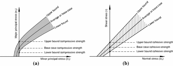
The strength of the damaged rock zone is bounded by lower and upper bounds. a Compressive strength curve in terms of principal stresses. b Shear strength curve obtained through the procedures described in step 2
By re-arranging Eq. 8a–c, the upper, lower and base case cohesive strengths can be calculated. In essence, the assumption is that, if ϕ = 0, then the shear strength of damaged rock will actually be equal to its cohesive strength according to the Mohr–Coulomb definition (τ = c + tanϕ). It is possible that, at low normal stresses (σ n < 1.0 MPa), the shear strength will indeed be the cohesive strength (see, for example, Saiang et al. 2005).


The three-step procedure shown above was used in estimating the values of the strength parameters for our models (see Table 3).
3.3 Modelling Scenarios
Table 4 shows the cases or scenarios modelled. The parameter studies (cases 3 to 7) were performed starting from the standard or base case model (Case 0). During each parameter test, a specified parameter is varied over a realistic range, while all other parameters are kept constant at their base case values. The mechanical parameters tests were only applied to the BIDZ. For the rock mass beyond the damaged zone (i.e. undamaged rock mass), the parameter values are kept constant at the values for the undamaged rock given in Table 3.
The base case model is based on 10 m of rock cover, which is typically the case in many railway tunnels in Sweden. The blast damaged zone is 0.5-m thick, with equal thickness around the tunnel. The input parameters for the base case model are those given in Table 3. The variable data set values for cases 2, 3 and 4 in the “High” column of Table 5 are the same values as for the undamaged rock.
For Case 7, the in-situ stresses were varied according to:
to assess the worst and best case scenarios. The maximum deviatoric stress scenario (Case 8) is when σ v is at its minimum, as per Eq. 9a, and σ h is at its maximum, as per Eq. 9c.
4 Results
The parameter analyses were conducted in line with the overall objective of the ongoing study on the mechanical behaviour of the blast-induced damaged rock around a tunnel boundary. By varying the mechanical properties of the damaged rock mass and other parameters (see Table 4), their effects were investigated in terms of variations in the magnitudes (and distribution) of the induced stresses and displacement vectors. The induced stresses were studied in terms of the differential stress (σ θ − σ r) magnitudes and distribution.
In order to see how the BIDZ affects the magnitude and distribution of the induced stresses, for given scenarios, observations were made at two points, A and B, in the tunnel roof, as shown in Fig. 11. Point A is located at/near the tunnel boundary, while Point B is located at the damaged–undamaged rock boundary. For the ground displacement magnitudes, measurements were taken from the tunnel wall (Point C) instead of the tunnel roof. This is because the displacement magnitudes were high in the tunnels walls and seemed to be clearly affected by the presence of the BIDZ.

Numerical measurement points around the tunnel where the differential stresses (σ θ − σ r) and displacement magnitudes were recorded
Figures 12 and 13 show the summary of the variations in the induced differential stress (σ θ − σ r ) and the ground deformation magnitudes, respectively, as the various parameters shown in Table 4 were varied. The variations at the tunnel boundary, Point A, are presented in terms of maximum percentage variations in Figs. 14 and 15, respectively. The percentage variations were calculated as maximum variations from the base case (i.e. Case 0) results. In the proceeding subsection, each of the parameters evaluated will be presented and discussed, while making references to these figures.

Differential stresses (σ θ − σ r) for the various scenarios tested. a Differential stresses on the tunnel boundary at Point A. b Differential stresses on the damaged–undamaged rock boundary at Point B

Ground displacement at the tunnel wall at Point C for the scenarios tested

Percentage variation in the differential stress at Points A and B for the scenarios tested

Percentage variation in displacement magnitudes at Point C for the scenarios tested
5 Discussions
5.1 Varying Deformation Modulus of the BIDZ
Varying the Young’s modulus of the BIDZ (E d) obviously affected the magnitude and distribution of the induced differential stresses (σ θ − σ r) around the tunnel boundary (see Figs. 12 and 13). For example, when E d was 50% of E m (Young’s modulus of the undamaged rock), the differential stress at Point A, in the tunnel roof, was reduced by 27% and at Point B by about 7% from the base case value (see Fig. 14). This can be a notable reduction in the confinement when stability and strength is concerned. There was also a corresponding increase in differential stresses at Point B (see Fig. 12b). This is obviously expected, as high stress magnitudes are diverted into the stiffer rock mass outside the BIDZ.
The observations seem to be consistent with some rule-of-thumb practices for boreholes and shafts where the E d at the borehole/shaft boundary is usually assumed to be about 50% of E m (Diederichs 2005; Malmgren et al. 2007) and the resulting variation in the induced stresses are usually as much as 30% (e.g. de la Vergne 2003).
The wall displacement varied by 30% when the stiffness of the damaged zone was reduced to 50% (see Fig. 15). A maximum displacement of 14 mm was observed in this case. This displacement may not be significant in practical cases, despite the fact that the stiffness of the damaged zone has been reduced by 50%. However, it can be critical in some cases, for example, if the tunnel is to be excavated in the vicinity of a pre-existing tunnel that hosts sensitive utilities.
5.2 Varying Compressive and Tensile Strengths
Varying the compressive strength of the BIDZ (σ d) apparently had no significant effect on the induced differential stress and ground deformation magnitudes (see Figs. 12–15). In a way, this can be expected, since the defined compressive strengths for the BIDZ and undamaged rock masses are much higher than the observed stress magnitudes. It can also be argued that the Mohr–Coulomb yield criteria may be vulnerable in accurately capturing the yield and failure process of brittle rocks under low confining stress conditions. Such arguments have been demonstrated by, for example, Martin et al. (1997), Hajiabdolmajid et al. (2002) and Diederichs (2003). Therefore, the results from the compressive strength simulation in this paper are not conclusive.
Evaluation of the yielded zones resulting from high and low compressive strengths of the BIDZ (see Table 5) appeared to be similar or unchanged (see Fig. 16). However, the yield zones appear to be affected by the variation in the tensile strength of the BIDZ (see Fig. 17). This effect is also reflected in Figs. 12–15, where the deviatoric stress and displacement magnitudes have been affected, although not very distinctively, since the tensile strength values used were small (see Table 5). Nevertheless, there is a clear indication that the tensile strength is a sensitive parameter for the conditions simulated.

Yielded zones when: a σ d = 26.8 MPa and b σ d = 8.8 MPa. There is no noticeable difference in the shape and extent of the yield zones for the two cases, except for minor shearing in the roof for the weaker rock mass case

Yielded zones when: a σ td = 0 MPa and b when σ td = 0.4 MPa. There is a recognisable difference in the size of the yield zones when σ td is increased from 0 to 0.4 MPa
The yielding also conforms well to the secondary stress distribution pattern (see Fig. 18). Regions A and B are where the tensile strength of the rock mass have been exceeded, leading to tensile yield patterns observed in Figs. 16 and 17. In region A, both principle stresses are in extension, with the value of σ 3 exceeding that of σ t (i.e. σ 3 < σ t and σ 1 < 0). In region B, σ 3 exceeds σ t, but σ 1 is greater than zero (i.e. σ 3 < σ t and σ 1 > 0).

Regions where the secondary stresses exceed the estimated tensile strength of the rock mass. Region A is where σ 3 < σ t and σ 1 < 0, and Region B is where σ 3 < σ t and σ 1 > 0
5.3 Varying Overburden
In this paper, shallow depth means an overburden thickness of less than 20 m. To be consistent with this definition, the overburden was varied between 2 and 20 m. The variations in the magnitudes of the induced differential stress for 2, 10 and 20 m overburden at points A and B (see Fig. 11) are shown in Figs. 12 and 14. It was observed that differential stress and displacement magnitudes at 10 m overburden were lower than those of 2 and 20 m overburden. To obtain a clear picture of this behaviour, the overburden was varied up to 500 m. The result is shown in Fig. 19. It can be seen that, for overburden greater than 10 m, the differential stress reaches a peak at about 200 m depth and, thereafter, there is not much variation, probably due to compressive yielding of the rock and, so, no further load can be sustained. It can be concluded that at depths less than 10 m, the rock mass above the tunnel behaves like a “cantilever beam,” thereby concentrating the stresses. At depths greater than 10 m, it behaves like a normal rock mass. Coincidently, the 10 m overburden in the standard model appears also to be the transition point of this phenomenon.

Effect of varying overburden on the differential stress at Point A on the tunnel boundary
5.4 Varying Damaged Zone Thickness
Variation in the thickness of the BIDZ appeared to have a minor effect on the differential stress and ground displacement magnitudes (see Figs. 12–15). The distribution of the differential stresses, however, was obvious, in that the peak stresses were pushed farther into the rock, resulting in the reduction of the peak value (see Fig. 12b) at the BIDZ boundary or Point B. The percentage variation in the differential stress at Point B is about 27% (see Fig. 14). The magnitudes of the differential stresses decrease with increasing BIDZ thickness, which is a phenomenon that is considered to be important in rock destressing practices (see, for example, Tang and Mitri 2001).
5.5 Varying in-situ Stresses
The base case model was tested at varying in-situ stresses as described by Eq. 9a–c. Three scenarios were tested: (1) maximum in-situ stresses, (2) minimum in-situ stresses and (3) maximum deviatoric in-situ stress [(σ H − σ v)max]. The results of the resulting displacements and induced stresses are shown among the bar charts of Figs. 12–15. Scenario (3) yielded induced differential stresses (σ θ − σ r) that were nearly the same amount as scenario (1). By percentage variation, the difference in (σ θ − σ r) at the tunnel boundary between scenarios (2) and (3) is about 51%, which is a significant variation in the (σ θ − σ r) magnitude. This implies that the presence of the BIDZ acts as a protective barrier against excessive stress accumulation near the tunnel boundary. Scenario (2) could pose a potentially unstable situation where excessive destressing may lead to low confinement, particularly in the roof, which could lead to other problems, such as the opening of cracks where water can easily flow in and out, and, thus, deteriorating the rock quality.
5.6 Ground Deformation
Figure 20 shows the general ground deformation pattern observed in the numerical study. The largest displacements occur in the tunnel walls, in the form of inward convergence, due to high horizontal stresses. In the tunnel roof, the deformation occurs in the form of roof divergence, leading to heaving directly above the tunnel roof. A maximum displacement of 14.0 mm was recorded on the tunnel wall when the E d was 50% of E m, whilst when E d = E m, it was 8.0 mm. In practical cases, a 14.0-mm ground displacement will most likely be considered to be insignificant, even though the stiffness of the rock mass has been reduced by half. The deformation observations (both in magnitude and pattern) are fairly consistent with the recent studies for the “Citybanan project” (Sjöberg et al. 2006), where the rock mass properties were similar to the ones used in this paper and were also located at shallow depths.

Typical ground deformation pattern observed
5.7 Classification of Parameter Sensitivity
Table 6 shows a classification of the sensitivity of the parameters tested. There is no specific criterion for this classification; it is purely based on how much the magnitude of the differential stresses and displacement vectors vary from the base case observations. The magnitudes of the variation are important in this case. For example, the magnitude of the displacement vectors is on the order of millimetres, which, in practical cases, will most likely be considered as negligible.
6 Conclusions
The presence of blast-induced damaged rock, or a BIDZ, clearly affected the distribution and magnitudes of induced boundary stresses and ground deformation. With various parameter combinations, such as, for example, low stiffness and high in-situ stress, the effect could become critical. However, any such criticality has to be studied objectively.
The magnitude and distribution of boundary stresses were also noted to be dependent on the mechanical and physical characteristics of the BIDZ. Of the parameters tested, the variation in the in-situ stresses affected both the differential stresses and displacement magnitudes the most. In terms of the inherent rock mechanical properties, the Young’s modulus affected the tangential stresses and displacements quite significantly when varied.
The effects due to variation in the compressive strength of the BIDZ are not conclusive. This may be due to several reasons, including the vulnerability of the method used in estimating strength parameter values and the possibility that the yield mechanism has not been accurately captured by the yield criterion used. Some authors (e.g. Cundall et al. 1996) suggested drastic reduction of the compressive strength to force failure when a Mohr–Coulomb yield criterion is used, but it is not clear which of the empirical strength components (c or ϕ) should be reduced. On the other hand, the tensile strength appeared to be sensitive for the conditions simulated. This is because the failure mechanisms observed appeared to be principally of tensile origin. To observe the post-peak behaviour, a strain-softening model with gradual reduction in the shear strength would be needed.
Although the results yielded useful conclusions about the effects of the BIDZ, the methods used in estimating the input parameters need further improvement. It was also evident that the usual method or the common practice approach for estimating the input parameters for the given rock mass conditions, using tools such as RocLab or the Hoek–Brown–GSI criterion directly, did not yield logical results.
Abbreviations
- σ i :
-
intact compressive strength (MPa)
- σ m :
-
compressive strength of the undamaged rock mass (MPa)
- E m :
-
deformation modulus of the undamaged rock mass (GPa)
- ϕ m :
-
frictional strength of the undamaged rock mass (°)
- c m :
-
cohesive strength of the undamaged rock mass (MPa)
- σ tm :
-
tensile strength of the undamaged rock mass (MPa)
- D :
-
disturbance factor
- σ d :
-
compressive strength of the damaged rock mass (MPa)
- E d :
-
deformation modulus of the damaged rock mass at the tunnel boundary (GPa)
- E d(ij) :
-
deformation modulus of the damaged rock mass at point i, j (GPa)
- ϕ d :
-
frictional strength of the damaged rock mass (°)
- c d :
-
cohesive strength of the damaged rock mass (MPa)
- σ td :
-
tensile strength of the damaged rock mass (MPa)
- L d :
-
total thickness of the damaged rock zone (m)
- L d(ij) :
-
thickness of the damaged rock zone at point i, j (m)
- σ UBd :
-
upper bound compressive strength of the damaged rock mass
- σ BCd :
-
base case compressive strength of the damaged rock mass
- σ LBd :
-
lower bound compressive strength of the damaged rock mass
- c UBd :
-
upper bound cohesive strength of the damaged rock mass
- c BCd :
-
base case cohesive strength of the damaged rock mass
- c LBd :
-
lower bound cohesive strength of the damaged rock mass
- σ θ − σ r :
-
induced differential or deviatoric stress
- σ θ :
-
tangential stress (induced)
- σ r :
-
radial stress (induced)
- σ 3max :
-
maximum confining stress
- σ 3min :
-
minimum confining stress
- σ nmax :
-
maximum normal stress derived from normal stress–shear stress envelope
- σ nmin :
-
minimum normal stress derived from normal stress–shear stress envelope
- τ max :
-
maximum shear stress derived from normal stress–shear stress envelope
- τ min :
-
minimum shear stress derived from normal stress–shear stress envelope
References
AnläggningsAMA-98 (1999) General materials and works description for construction work, section CBC: Bergschakt (in Swedish). Svensk Byggtjäanst, Stockholm
Banverket (2002) BV Tunnel. Standard BVS 585.40. Banverket
Barla G, Barla M, Repetto L (1999) Continuum and discontinuum modelling for design analysis of tunnels. In: Proceedings of the 9th international congress on rock mechanics, Paris, France, August 1999
Brown ET (ed) (1981) ISRM commission on standardization of laboratory and field tests. Suggested methods for the quantitative description of discontinuities in rock masses. Pergamon Press
Cundall PA, Potyondi DO, Lee CA (1996) Micromechanics-based models for fracture and breakout around the mine-by tunnel. In: Martino JB, Martin CD (eds) Proceedings of the excavation disturbed zone (EDZ) workshop—designing the excavation disturbed zone for a nuclear waste repository in hard rock, Winnipeg, Manitoba, Canada, September 1996, pp 113–122
da Gama CD (ed) (1998) Quantification of rock damage for tunnel excavation by blasting. Tunnels and metropolises. Balkema, Rotterdam, pp 451–456
de la Vergne JN (2003) Hard rock miner’s handbook. McIntosh engineering, Tempe, AZ, p 262
Diederichs MS (2003) Rock fracture and collapse under low confinement conditions. Rock Mech Rock Eng 36(5):339–381
Diederichs MS (2005) Personal communication
Diederichs MS, Kaiser PK (1999) Tensile strength and abutment relaxation as failure control mechanisms in underground excavations. Int J Rock Mech Min Sci 36(1):69–96
Farmer IW (1968) Engineering properties of rocks. E. & F.N. Spon Ltd., p 180
Feng X-T, Zhang Z, Sheng Q (2000) Estimating mechanical rock mass parameters relating to the Three Gorges Project permanent shiplock using an intelligent displacement back analysis method. Int J Rock Mech Min Sci 37(7):1039–1054
Fjellborg S, Olsson M (1996) Long drift rounds with large cut holes at LKAB. SveBeFo Report No. 27, Swedish Rock Engineering Research, Stockholm
Forsyth WW, Moss AE (eds) (1991) Investigation of development blasting practices. CANMET-MRL, pp 91–143
Hajiabdolmajid V, Kaiser PK, Martin CD (2002) Modeling brittle failure of rock. Int J Rock Mech Min Sci 39(6):731–741
Hoek E (2007) Practical rock engineering. Available online at: http://www.rocscience.com/hoek/PracticalRockEngineering.asp
Hoek E, Diederichs MS (2006) Empirical estimation of rock mass modulus. Int J Rock Mech Min Sci 43(2):203–215
Hoek E, Kaiser PK, Bawden WF (1995) Support for underground excavations in hard rock. A.A. Balkema, Rotterdam, p 215
Hoek E, Carranza-Toress C, Corkum B (2002) Hoek–Brown failure criterion—2002 edition. In: Proceedings of 5th North American rock mechanics symposium and the 17th Tunnelling Association of Canada conference (NARMS-TAC 2002), University of Toronto, Canada, July 2002, pp 267–271
Holmberg R (1982) Charge calculation for tunneling. In: Hustrulid W (ed) Underground mining methods handbook. Society of Mining Metallurgy and Exploration, Littleton, pp 1580–1589
Holmberg R, Persson P-A (1980) Design of tunnel perimeter blasthole patterns to prevent rock damage. Trans Inst Min Metall 89:A37–A40
Hustrulid W (1994) The “practical” blast damage zone in drift driving at the Kiruna mine. In: Proceedings of the seminar Skadezon vid tunneldrivning, SveBeFo, Stockholm
Itasca (2002) FLAC version 4.00. Itasca Consulting Group, Minneapolis
Ladegaard-Pedersen A, Daly JW (1975) A review of factors affecting damage in blasting. Mechanical Engineering Department, University of Maryland
Lundman P (2004) Personal communication
MacKown AF (1986) Perimeter controlled blasting for underground excavations in fractured and weathered rocks. Bull Assoc Eng Geol XXIII(4):461–478
Malmgren L, Saiang D, Töyrä J, Bodare A (2007) The excavation disturbed zone (EDZ) at Kiirunavaara mine, Sweden—by seismic measurements. J Appl Geophys 61(1):1–15
Martin CD, Read RS, Martino JB (1997) Observations of brittle failure around a circular test tunnel. Int J Rock Mech Min Sci 34(7):1065–1073
Martino JB (2003) The 2002 international EDZ workshop: the excavation damaged zone—cause and effects, Atomic Energy of Canada Limited
Martino JB, Martin CD (1996) Proceedings of the excavation disturbed zone workshop, Manitoba
Nyberg U, Fjellborg S (2002) Controlled drifting and estimating blast damage. In: Holmberg R (ed) Proceedings first world conference on explosives and blasting technique. Balkema, Rotterdam, pp 207–216
Olsson M, Bergqvist I (1993) Crack lengths from explosives in small diameter holes. SveBeFo Report No. 3, Swedish Rock Engineering Research, Stockholm
Olsson M, Bergqvist I (1995) Crack propagation in rock from multiple hole blasting—part 1. SveBeFo Report No. 18, Swedish Rock Engineering Research, Stockholm
Olsson M, Bergqvist I (1997) Crack propagation in rock from multiple hole blasting—summary of work during the period 1993–96. SveBeFo Report No. 32, Swedish Rock Engineering Research, Stockholm
Olsson M, Ouchterlony F (2003) New formula for blast induced damage in the remaning rock. SveBeFo Report No. 65, Swedish Rock Engineering Research, Stockholm
Oriad LL (1982) Blasting effect and their control. In: Hustrulid W (ed) Underground mining methods handbook. Society of Mining Engineers of AIME, New York, pp 1590–1603
Ouchterlony F (1997) Prediction of crack lengths in rock after cautious blasting with zero inter-hole delay. SveBeFo Report No. 31, Swedish Rock Engineering Research, Stockholm
Ouchterlony F, Olsson M, Bergqvist I (2001) Towards new Swedish recommendations for cautious perimeter blasting. Explo 2001. Hunter Valley, NSW
Pelli F, Kaiser PK, Morgenstern NR (1991) The influence of near face behaviour on monitoring of deep tunnels. Can Geotech J 28(2):226–238
Persson P-A, Holmberg R, Lee J (1996) Rock blasting and explosives engineering. CRC Press, Tokyo, pp 265–285
Plis MN, Fletcher LR, Stachura VJ, Sterk PV (1991) Overbreak control in VCR stopes at Homestake mine. In: 17th Conference on explosives and blasting research, ISEE, pp 1–9
Priest SD (2005) Determination of shear strength and three-dimensional yield strength for the Hoek–Brown criterion. Rock Mech Rock Eng 38(4):299–327
Pusch R, Stanfors R (1992) The zone of disturbance around blasted tunnels at depth. Int J Rock Mech Min Sci Geomech Abstr 29(5):447–456
Raina AK, Chakraborty AK, Ramulu M, Jethwa JL (2000) Rock mass damage from underground blasting, a literature review, and lab- and full scale tests to estimate crack depth by ultrasonic method. FRAGBLAST Int J Blast Fragm 4:103–125
Ricketts TE (1988) Estimating underground mine damage produced by blasting. In: 4th Mini symposium on explosive and blasting research, Society of Explosive Engineers, Anaheim, CA, pp 1–15
Robertson AM (1973) Determination of joint populations and their significance for tunnel stability. Trans Soc Min Eng AIME 254(2):135–139
Rocscience (2002) RocLab, Rocscience Inc.
Saiang D (2004) Damaged rock zone around excavation boundaries and its interaction with shotcrete. Licentiate Thesis, Luleå University of Technology, p 121
Saiang D, Malmgren L, Nordlund E (2005) Laboratory tests on shotcrete-rock joints in direct shear, tension and compression. Rock Mech Rock Eng 38(4):275–297
Sato T, Kikuchi T, Sugihara K (2000) In-situ experiments on an excavation disturbed zone induced by mechanical excavation in Neogene sedimentary rock at Tono mine, central Japan. Eng Geol 56(1–2):97–108
Sheng Q, Yue ZQ, Lee CF, Tham LG, Zhou H (2002) Estimating the excavation disturbed zone in the permanent shiplock slopes of the Three Gorges Project, China. Int J Rock Mech Min Sci 39(2):165–184
Sjöberg J, Perman F, Leaner M, Saiang D (2006) Three-dimensional analysis of tunnel intersections for a train tunnel under Stockholm. In: Proceedings of the 2006 North American Tunneling conference, Chicago, Illinois, June 2006
Stephansson O (1993) Rock stress in the Fennoscandian shield. In: Hudson JA (ed) Comprehensive rock engineering. Pergamon Press, Oxford, pp 445–459
Tang B, Mitri HS (2001) Numerical modelling of rock preconditioning by destress blasting. J Ground Improv 5(2):57–67
Töyrä J (2006) Behaviour and stability of shallow underground constructions. Licentiate Thesis, Luleå University of Technology, Luleå, p 135
Whittaker BN, Singh RN, Sun G (1992) Rock fracture mechanics—principles, design and applications. Developments in geotechnical engineering, vol 71. Elsevier, Amsterdam, p 568
Yang RL, Rocque P, Katsabanis P, Bawden WF (1993) Blast damage study by measurement of blast vibration and damage in the area adjacent to blast hole. In: Rossmanith HP (ed) Rock fragmentation by blasting. Balkema, Rotterdam
Acknowledgements
The authors wish to acknowledge the Swedish Railroad Administration (Banverket) for funding this study, and Mr. Peter Lundman and Dr. Finn Ouchterlony for discussing the tunnel and rock excavation guidelines in Sweden. Doctors Evert Hoek and Mark Diederichs are sincerely acknowledged for their communications regarding the use of the Hoek–Brown criterion for shallow excavations and the use of disturbance factor descriptions for estimating the deformation modulus for the damaged rock.
Author information
Authors and Affiliations
Corresponding author
Rights and permissions
About this article
Cite this article
Saiang, D., Nordlund, E. Numerical Analyses of the Influence of Blast-Induced Damaged Rock Around Shallow Tunnels in Brittle Rock. Rock Mech Rock Eng 42, 421–448 (2009). https://doi.org/10.1007/s00603-008-0013-1
Received:
Accepted:
Published:
Issue Date:
DOI: https://doi.org/10.1007/s00603-008-0013-1