Relaxation of a scalar nonlocal variational problem with a double-well potential

Abstract

We consider nonlocal variational problems in $L^p$, like those that appear in peridynamics, where the functional object of the study is given by a double integral. It is known that convexity of the integrand implies the lower semicontinuity of the functional in the weak topology of $L^p$. If the integrand is not convex, a usual approach is to compute the relaxation, which is the lower semicontinuous envelope in the weak topology. In this paper we compute such a relaxation for a scalar problem with a double-well integrand. The relaxation is non-trivial, and, contrary to the local case, it cannot be represented as a double integral, as the original problem. Nonetheless, we show that, as for the local case, the relaxation can be expressed in terms of the energy of a suitable truncation of the considered function.

1 Introduction

The object of this paper are functionals I of the form

(1.1)

where $\varOmega \subset {\mathbb {R}}^n$ is a bounded open subset, $u : \varOmega \rightarrow {\mathbb {R}}$ is in some Lebesgue space $L^p$ with $1< p < \infty$, and the integrand $w :\varOmega \times \varOmega \times {\mathbb {R}} \times {\mathbb {R}}\rightarrow {\mathbb {R}}$ satisfies some natural regularity, coercivity and growth conditions. The symbol indicates the integral divided by the measure of $\varOmega$; the use of the average integral is just a convenient normalization. This kind of functionals represents an energy and appears in many contexts in the modelling of some nonlocal processes, such as peridynamics [37], phase transitions [2], pattern formation [21], image processing [23] and diffusion [4]. Our main motivation comes from peridynamics: in such a context, $\varOmega$ represents the reference configuration of a solid which undergoes a deformation u, and I measures the energy of that deformation. The nonlocal behavior comes from the fact that the energy density takes into account the interaction between all points of the body.

A usual procedure for showing the existence of minimizers of the energy functional I is the direct method of the Calculus of variations, whose main ingredients are coercivity and lower semicontinuity. The natural topology in this context is the weak topology in $L^p$, since it is in this case where the coercivity implies the compactness. The works [10, 11, 13, 20, 33] deal precisely with the issue of existence of minimizers, and, as a part of the study, they analyze necessary and sufficient conditions for the lower semicontinuity of I in the weak topology of $L^p$. One of such necessary and sufficient conditions involves a nonlocal property of convexity which is difficult to understand, even for $n=1$; see [12, 19, 29]. Nevertheless, when the integrand $w = w(x, x', y, y')$ does not depend on $(x, x')$, and the dependence on $(y, y')$ is through the difference $y-y'$, i.e., when, given a function $f : {\mathbb {R}} \rightarrow {\mathbb {R}}$, the energy functional is

(1.2)

such a nonlocal property of convexity is equivalent to convexity of f: see, e.g., [11, Sect. 7].

Thus, if f is not convex, the functional I is not lower semicontinuous in the weak topology of $L^p$. A usual approach to tackle this obstacle is to consider the relaxation $I^*$, which consists in finding the lower semicontinuous envelope of I. In the classical local context of nonlinear elasticity, understanding the relaxation is capital to study the microstructure of the material [8], although in this nonlocal context the relaxation has a slightly different interpretation in terms of microstructure, as will be seen in Sect. 10.

Relaxation for nonlocal functionals similar to I but depending on $\nabla u$ was analyzed in [12, 19, 29, 30]. These works study necessary and sufficient conditions for the weak lower semicontinuity, as well as abstract relaxation functionals, but they do not compute the lower semicontinuous envelope of the considered functional. The article [11], on the other hand, analyzes the relaxation of the functional I in terms of Young measures, which are, roughly speaking, families of probability measures parametrized by $x \in \varOmega$ that capture the information of the possible oscillations of sequences converging weakly in $L^p (\varOmega )$.

In this paper we compute the relaxation $I^*$ of I for a particular, but paradigmatic, case of non-convex f; namely,

$$\begin{aligned} f(t)=-2\alpha t^2+t^4, \qquad \alpha >0, \end{aligned}$$

(1.3)

one of the most used double-well potentials for modelling phase transitions. For such an integrand, we give an explicit formula for the relaxation which allows us, among other results, to solve the question, in the negative, of the integral representation for the relaxed functional, i.e., we show that there does not exist any function g such that $I^*(u)$ can be written in the form

(1.4)

Such a result was suggested in [11, 33] but its proof was left open. Moreover, even though for this f the functional I(u) only depends on the second and fourth moments of u (see Sect. 6), its relaxation $I^*$ cannot be written as a function depending on those moments.

The main steps of the proof are the following:

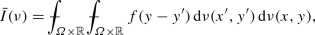
• (i) We start with the result of Bellido and Mora-Corral [11], which states that the relaxation of I in the space of Young measures is the functional ${\bar{I}}$ defined in the space of Young measures in $\varOmega \times {\mathbb {R}}$ as

  

  and show (see Proposition 4.1) that $I^* (u)$ can be characterized as the minimum of ${\bar{I}} (\nu )$ among Young measures $\nu$ with barycenter u. This result is totally analogous to classical results in local problems.

• (ii) In Propositions 5.1 and 5.2 , where we consider a general integrand w, we obtain (first and second order) optimality conditions satisfied by any measure $\nu$ that solves the minimization problem of Step  i). To do so, we adapt the method of Pedregal [32], who established optimality conditions for a problem defined in the set of Young measures with no restrictions. Since the original problem in [32] contains $\nabla u$, the analysis was limited to $n=1$. Here, we obtain optimality conditions for any $n\ge 1$, and, in addition, we incorporate the restriction that the barycenter of $\nu$ has to be u.

  Later, an analysis of our optimality conditions for the specific f given in (1.3) allows us to conclude (see Steps 1–3 in the proof of Theorem 6.2) that the optimal Young measure has the form

  $$\begin{aligned} \nu _x={\left\{ \begin{array}{ll} \delta _{u(x)} &{} \text {for } x\in \varOmega _1, \\ \frac{v_2(x)-u(x)}{v_2(x)-v_1(x)} \delta _{v_1(x)}+\frac{u(x)-v_1(x)}{v_2(x)-v_1(x)} \delta _{v_2(x)} &{} \text {for } x\in \varOmega _2. \end{array}\right. } \end{aligned}$$

  for some disjoint sets $\varOmega _1, \varOmega _2$ with union $\varOmega$ and some functions $v_1, v_2$.

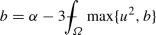
• (iii) We do variations of the $v_1$ and $v_2$ and conclude that $v_1 + v_2 = 0$ and $v_1$ and $v_2$ are constant (see Steps 4–5 in the proof of Theorem 6.2). Moreover, $v_1^2 = v_2^2 = b_u$ where $b_u$ is the only solution $b>0$ to the equation

  

  (see Sect. 7).

• (iv) We do variations of $\varOmega _1$ and conclude that $\varOmega _1$ is the set where $u^2 \ge b_u$ (see Step 6 in the proof of Theorem 6.2). Thus, $\nu$ is completely determined, $I^* (u) = {\bar{I}} (\nu )$ and, in fact,

  $$\begin{aligned} I^* (u) = I \left( \max \left\{ |u| , \sqrt{\max \{ b_u, 0 \}} \right\} \right) \end{aligned}$$

  (1.5)

  (see Theorem 7.2 and Corollary 7.3).

It is worth noticing that, even though Young measures are extensively used in the characterization of $I^*$, our final formula for $I^*$ does not involve Young measures, as can be seen from (1.5).

The impossibility of expressing $I^*$ as a functional of the style (1.4) represents a remarkable difference with the local case. Nevertheless, there are also some similitudes, since, as formula (1.5) shows and will be explained in Sect. 10, both local and nonlocal relaxations can be obtained through a suitable truncation of u.

We mention two relevant works related to ours: [25, 26]. In [26], lower semicontinuity and relaxation for nonlocal problems are also studied, but in the context of $L^{\infty }$. In such a work the functional involves the essential supremum and the authors show that the relaxed functional has the same structure as the original one (with another supremand), a remarkable difference with our negative representation result (see Proposition 9.1). A follow-up of [26] is [25], where they show that, in general, the relaxation in $L^p$ of functionals I of the style of (1.1) is not given by a double integral. They also show instances where the relaxation does preserve the structure of a double integral. Their approach is very different from ours and is based on the study of nonlocal inclusions.

Although the relaxation is determined here for the specific f given in (1.3), we believe that the same techniques can be used to compute the relaxation for I in (1.2) when f is a $C^2$ even function with a typical profile of a double-well potential. However, the relaxation of I for an integrand depending explicitly on $(x,x')$ seems to be substantially more difficult, as does the vectorial case (when u takes values in ${\mathbb {R}}^d$).

This paper is organized as follows. Section 2 presents some definitions about Young measures in $L^p$. In Sect. 3 we review the results of [11], which shows the formula for ${\bar{I}}$, the relaxation of I in the space of Young measures. In Sect. 4 we prove an abstract formula for $I^*$ in terms of ${\bar{I}}$, namely, $I^* (u)$ is the minimum of ${\bar{I}} (\nu )$ among the Young measures $\nu$ with barycenter u. In the same section we also review the necessary and sufficient conditions for I to be lower semicontinuous in the weak topology of $L^p$. In Sect. 5 we adapt the method of [32] to find optimality conditions for the Young measures that minimize ${\bar{I}}$, for general $n\ge 1$ and under the constraint that their barycenter is u. The core of the paper are Sects. 6 and 7 . For the particular case of (1.2) when f is given by (1.3), we give in Sect. 6 a complete description of the Young measures with given barycenter that minimize ${\bar{I}}$. Using this result, in Sect. 7 we compute $I^*$. Section 8 illustrates the relaxation result of Sect. 7 to compute $I^* (u)$ for particular examples of u, while in Sect. 9 we use such examples to show that $I^*$ is not given by a functional of the form (1.4) or by a function depending only on the second and fourth moments of u. Finally, in Sect. 10, we compare our relaxation formula with that of the local case, and give an interpretation in terms of the microstructure of the deformed material.

2 Young measures in $L^p$

In this section we briefly recall the definitions and results concerning Young measures that are needed in the paper; for the proofs and general expositions, we refer the reader to [5,6,7, 11, 22, 31, 38, 39].

We start with some general notation of measure theory. Throughout the paper, $\varOmega$ denotes a non-empty bounded open set of ${\mathbb {R}}^n$, $n\ge 1$; from Sect. 3 it will be assume to be connected (so, a domain) and with a Lipschitz boundary.

We will use both Lebesgue and Borel measurability: Lebesgue measurability will be in a Lebesgue measurable subset of ${\mathbb {R}}^n$, while Borel measurability will be in ${\mathbb {R}}$. The Lebesgue measure in ${\mathbb {R}}^n$ will be denoted by $\mathcal {L}^n$; the Lebesgue measure of a measurable $E \subset {\mathbb {R}}^n$ is denoted by $\mathcal {L}^n (E)$ or |E|. When we just write measurable, it means Lebesgue measurable, while, when we say $\mathcal {B}$-measurable, it means Borel measurable. Likewise, $\mathcal {L}^n \otimes \mathcal {B}$-measurable means measurable in $\varOmega \times {\mathbb {R}}$ with respect to the product measure. In fact, the paper deals with functions defined either in $\varOmega \times \varOmega \times {\mathbb {R}} \times {\mathbb {R}}$ (in which case we assume $\mathcal {L}^{2n} \otimes \mathcal {B}^2$-measurability) or in ${\mathbb {R}}$ (in which case we assume $\mathcal {B}$-measurability). In the notation of the introduction, these two cases correspond to the integrands $w = w (x, x', y, y')$ and $w = f (y-y')$.

Given a measurable set E and $1 \le p < \infty$, the Lebesgue space $L^p(E)$ is defined in the usual way. Weak convergence in $L^p$ is denoted by $\rightharpoonup$.

Given $a \in {\mathbb {R}}$, the Dirac delta at a is denoted by $\delta _a$, while the average integral $\fint _E$ denotes the integral in E divided by $\mathcal {L}^n (E)$.

Given $E \subset {\mathbb {R}}^n$, C(E) is the set of continuous functions in E. Its subset of bounded functions is denoted by $C_b (E)$, and is endowed with the supremum norm $\left\| \cdot \right\| _{\infty }$. In addition, $C_0 (E)$ is its subset of functions u such that for every $\varepsilon >0$ there exists a compact $K \subset E$ such that $|u(x)| < \varepsilon$ for all $x \in E \setminus K$.

A Young measure in $\varOmega \times {\mathbb {R}}$ is a measure $\nu$ in $\varOmega \times {\mathbb {R}}$, equipped with the $\mathcal {L}^n \otimes \mathcal {B}$-sigma algebra, such that for any measurable $E \subset \varOmega$,

$$\begin{aligned} \nu (E \times {\mathbb {R}}) = \mathcal {L}^n (E) . \end{aligned}$$

We denote by $\mathcal {Y} (\varOmega )$ the set of Young measures in $\varOmega \times {\mathbb {R}}$.

Thanks to the procedure of disintegration (or slicing; see, e.g., [6, Th. 4.2.4]), any $\nu \in \mathcal {Y} (\varOmega )$ can be identified with a family $\left( \nu _x \right) _{x \in \varOmega }$ of probability measures on ${\mathbb {R}}$ such that for all $f \in C_0 (\varOmega \times {\mathbb {R}})$, the map

$$\begin{aligned} \varOmega \ni x \mapsto \int _{{\mathbb {R}}} f(x, y) \, \mathrm {d}\nu _x (y) \end{aligned}$$

is measurable and

$$\begin{aligned} \int _{\varOmega \times {\mathbb {R}}} f (x, y) \, \mathrm {d}\nu (x, y) = \int _{\varOmega } \left( \int _{{\mathbb {R}}} f(x, y) \, \mathrm {d}\nu _x (y) \right) \mathrm {d}x . \end{aligned}$$

Thus, we write $\nu = \left( \nu _x \right) _{x \in \varOmega }$. In the sequel, we will use both approaches.

Any measurable function $u : \varOmega \rightarrow {\mathbb {R}}$ can be identified with the Young measure $\nu ^u = \left( \nu ^u_x \right) _{x \in \varOmega }$ given by $\nu ^u_x = \delta _{u(x)}$ for all $x\in \varOmega$, i.e.,

$$\begin{aligned} \int _{\varOmega \times {\mathbb {R}}} \varphi (x, y) \, \mathrm {d}\nu ^u (x, y) = \int _{\varOmega } \varphi (x, u(x)) \, \mathrm {d}x \end{aligned}$$

for all $\varphi \in C_0 (\varOmega \times {\mathbb {R}})$. With a small abuse of notation, we write $u \in \mathcal {Y} (\varOmega )$.

Given $p \ge 1$, we denote by $\mathcal {Y}^p (\varOmega )$ the set of $\nu \in \mathcal {Y} (\varOmega )$ such that

$$\begin{aligned} \int _{\varOmega \times {\mathbb {R}}} |y|^p \, \mathrm {d}\nu (x, y) < \infty . \end{aligned}$$

As a consequence of Hölder’s inequality, $\mathcal {Y}^p (\varOmega ) \subset \mathcal {Y}^q (\varOmega )$ if $1 \le q \le p$.

3 Relaxation in the set of Young measures

In this section we recall some results of [11] that will be used later. Given a function $w : \varOmega \times \varOmega \times {\mathbb {R}} \times {\mathbb {R}} \rightarrow {\mathbb {R}}$, it is said to be symmetric if $w(x,x',y,y')=w(x',x,y',y)$ for a.e. $x, x'\in \varOmega$ and all $y, y'\in {\mathbb {R}}$. We say that w is Carathéodory if it is $\mathcal {L}^{2n} \otimes \mathcal {B}^2$-measurable and for a.e. $x, x' \in \varOmega$, the function $w (x, x', \cdot , \cdot )$ is continuous.

We fix $p>1$ and define the functional I in $L^p (\varOmega )$ as in (1.1). In this work, no boundary conditions are imposed, although a slight variant of the proofs can easily deal with them; in any case, boundary conditions in a nonlocal context are different from the usual Dirichlet or Neumann conditions in a local setting; see, e.g., [11]. We assume that the problem is invariant under translations, i.e., $I(u) = I(u+a)$ for all $u \in L^p (\varOmega )$ and $a \in {\mathbb {R}}$. This is the case, for example, if w depends on y and $y'$ only through the difference $y-y'$, as we will assume from Sect. 6. Thus, we can assume, without loss of generality, that $\int _{\varOmega } u = 0$. We denote by $L^p_0 (\varOmega )$ the set of $u \in L^p (\varOmega )$ such that $\int _{\varOmega } u = 0$. Accordingly, our problem is to calculate the relaxation $I^*$ of (1.1) in the weak topology of $L^p_0 (\varOmega )$.

Given $\nu \in \mathcal {Y}^p (\varOmega )$ and $i\in {\mathbb {N}}$ with $i \le p$, we define its ith moment $M_i (\nu )$ as the measurable function $M_i (\nu ) : \varOmega \rightarrow {\mathbb {R}}$

$$\begin{aligned} M_i (\nu ) (x) := \int _{{\mathbb {R}}} y^i \, \mathrm {d}\nu _x (y) . \end{aligned}$$

Jensen’s (or Hölder’s) inequality shows at once that $M_i (\nu ) \in L^{\frac{p}{i}} (\varOmega )$.

The first result that we recall from [11] gives the relaxation of I in $\mathcal {Y}^p (\varOmega )$. The precise statement is the following, where we denote by $\chi _{B(0, \delta )}$ the characteristic function of the ball $B(0, \delta )$ of ${\mathbb {R}}^n$.

Theorem 3.1

([11], Th. 6.3) Let $\varOmega$ be a Lipschitz domain of ${\mathbb {R}}^n$, fix $\delta > 0$ and let $p > 1$. Assume $w : \varOmega \times \varOmega \times {\mathbb {R}} \times {\mathbb {R}} \rightarrow {\mathbb {R}}$ is symmetric, Carathéodory and there exist $a_1, a_2 \in L^1 (\varOmega \times \varOmega )$ and $c>0$ such that

$$\begin{aligned} a_1(x,x') + \frac{1}{c} \chi _{B(0, \delta )} (x-x') \left| y-y' \right| ^p \le \left| w(x, x', y, y') \right| \le a_2(x, x') + c \left( \left| y \right| ^p + \left| y' \right| ^p \right) , \end{aligned}$$

(3.1)

for a.e. $x, x' \in \varOmega$ and all $y, y' \in {\mathbb {R}}$. Let $\mathcal {Y}^{p,0} (\varOmega )$ be the set of $\nu \in \mathcal {Y}^p (\varOmega )$ whose first moment u lies in $L^p_0(\varOmega )$. Define $I_1 , {\bar{I}} : \mathcal {Y}^p (\varOmega ) \rightarrow {\mathbb {R}} \cup \{\infty \}$ as

$$\begin{aligned} I_1 (\nu )&:= {\left\{ \begin{array}{ll} I (u) &{} \text {if } \nu = \left( \delta _{u (x)} \right) _{x \in \varOmega } \text { for some } u \in L^p_0 (\varOmega ) , \\ \infty &{} \text {otherwise,} \end{array}\right. } \\ {\bar{I}} (\nu )&:= {\left\{ \begin{array}{ll} \displaystyle \int _{\varOmega \times {\mathbb {R}}} \int _{\varOmega \times {\mathbb {R}}} w (x, x', y, y') \, \mathrm {d}\nu (x, y) \, \mathrm {d}\nu (x', y') &{} \text {if } \nu \in \mathcal {Y}^{p,0} (\varOmega ) ,\\ \infty &{} \text {otherwise.} \end{array}\right. } \end{aligned}$$

Then, the lower semicontinuous envelope of $I_1$ with respect to the narrow topology is ${\bar{I}}$.

We point out that the term $|y'|^p$ in the right-hand side of (3.1) was mistakenly missed out in [11]. Theorem 3.1 mentions the narrow topology for Young measures: we refer to [11] or general references on Young measures [5,6,7, 22, 31, 38, 39] for its definition, because it is not essential here; indeed, it is only used in the proof of Proposition 4.1 below.

A second key result that we will need is the following nonlocal Poincaré inequality. It has been proved, with different versions, in [14, 15, Th. 1], [34, Th. 1.1], [3, Prop. 4.1], [1, Cor. 3.4] and [24, Cor. 4.6]. The following formulation is taken from [10, Prop. 4.2] and [11, Prop. 4.3].

Proposition 3.2

([11], Prop. 4.3) Let $\varOmega$ be a Lipschitz domain of ${\mathbb {R}}^n$, fix $\delta > 0$ and let $p \ge 1$. Then there exists $\lambda >0$ such that for all $u \in L^p_0 (\varOmega )$,

$$\begin{aligned} \int _{\varOmega } \left| u (x) \right| ^p \, \mathrm {d}x \le \lambda \int _{\varOmega } \int _{\varOmega \cap B (x, \delta )} \left| u (x) - u (x') \right| ^p \, \mathrm {d}x' \, \mathrm {d}x . \end{aligned}$$

4 Relaxation in $L^p$

As mentioned in the previous sections, we denote by $I^*$ the lower semicontinuous envelope of I in the weak topology of $L^p_0 (\varOmega )$, i.e., $I^*$ is the greatest lower semicontinuous function in $L^p_0 (\varOmega )$ that is below I:

$$\begin{aligned} I^* := \sup \bigl \{ J :\ J :L^p_0 (\varOmega ) \rightarrow {\mathbb {R}} \text { is l.s.c. in the weak topology and } J \le I \bigr \} . \end{aligned}$$

Condition (3.1) and Proposition 3.2 imply at once that, for any $u \in L^1_0 (\varOmega )$, the quantity I(u) is well defined and finite if and only if $u \in L^p (\varOmega )$. In fact, given a subset $\mathcal {A} \subset L^p_0 (\varOmega )$, we have that $\mathcal {A}$ is bounded in $L^p (\varOmega )$ if and only if $\{ I (u) : u \in \mathcal {A} \}$ is bounded. As a consequence, in order to calculate $I^*$ it suffices to consider bounded sets in $L^p_0 (\varOmega )$. As bounded sets in the weak topology are metrizable (see, e.g., [16, Th. 3.29]), the topology in those sets $\mathcal {A}$ is metrizable. In particular (see, e.g., [6, Th. 11.1.1] or [22, Prop. 3.12]), for any $u \in L^p_0 (\varOmega )$,

$$\begin{aligned} I^* (u) = \inf \left\{ \liminf _{j \rightarrow \infty } I (u_j) : \ \{ u_j\}_{j \in {\mathbb {N}}} \subset L^p_0 (\varOmega ) \ \text { and } \ u_j \rightharpoonup u \text { as } j \rightarrow \infty \right\} \end{aligned}$$

and, moreover, we have that a functional $I^*$ is the relaxation of I if and only if:

• (i) For any sequence $\{ u_j \}_{j \in {\mathbb {N}}}$ in $L^p_0 (\varOmega )$ such that $u_j \rightharpoonup u$ as $j \rightarrow \infty$ for some $u \in L^p_0 (\varOmega )$, we have

  $$\begin{aligned} I^* (u) \le \liminf _{j \rightarrow \infty } I (u_j). \end{aligned}$$

• (ii) For any $u \in L^p_0 (\varOmega )$ there exists a sequence $\{ u_j \}_{j \in {\mathbb {N}}}$ in $L^p_0 (\varOmega )$ such that $u_j \rightharpoonup u$ as $j \rightarrow \infty$ and

  $$\begin{aligned} I^* (u) = \lim _{j \rightarrow \infty } I (u_j). \end{aligned}$$

Although $\varGamma$-convergence is not used in this paper, we mention that the relaxation $I^*$ is nothing but the $\varGamma$-limit of the constant sequence I.

Given $u \in L^p_0 (\varOmega )$, we denote by $\mathcal {Y}^p_u (\varOmega )$ the set of $\nu \in \mathcal {Y}^p (\varOmega )$ such that $M_1 (\nu ) = u$.

We are now able to give the result that establishes the relation between $I^*$ and the functional ${\bar{I}}$ introduced in Theorem 3.1; it shows a total analogy with the local case (see, e.g., [22, Th. 8.20]) and will be the starting point for our analysis. As pointed out above, its proof is the only place in the article where narrow convergence of Young measures is actually used and we send the reader to any of [5,6,7, 11, 22, 31, 38, 39] for its definition and properties.

Proposition 4.1

Let $w : \varOmega \times \varOmega \times {\mathbb {R}} \times {\mathbb {R}} \rightarrow {\mathbb {R}}$ satisfy the same assumptions of Theorem 3.1. Then, for every $u \in L^p_0 (\varOmega )$,

$$\begin{aligned} I^* (u) = \min \left\{ {\bar{I}}(\nu ) : \, \nu \in \mathcal {Y}^p_u (\varOmega ) \right\} . \end{aligned}$$

Proof

Let $u \in L^p_0 (\varOmega )$ and denote by $m_u$ the infimum of $\left\{ {\bar{I}}(\nu ) : \, \nu \in \mathcal {Y}^p_u (\varOmega ) \right\}$. We first show that this infimum is attained, so it is in fact a minimum. Condition (3.1) shows that $m_u \in {\mathbb {R}}$. Let $\{ \nu _j \}_{j \in {\mathbb {N}}}$ be a sequence in $\mathcal {Y}^p_u (\varOmega )$ such that ${\bar{I}} (\nu _j) \rightarrow m_u$ as $j \rightarrow \infty$. Then, $\{ {\bar{I}} (\nu _j) \}_{j \in {\mathbb {N}}}$ is bounded, and, by (3.1) and Proposition 3.2, we have that

$$\begin{aligned} \sup _{j \in {\mathbb {N}}} \int _{\varOmega \times {\mathbb {R}}} |y|^p \, \mathrm {d}\nu ^j (x, y) < \infty . \end{aligned}$$

According to the criterion of tightness for Young measures (see, e.g., [11, Th. 3.3]), there exists $\nu \in \mathcal {Y} (\varOmega )$ such that, for a subsequence, $\{ \nu _j \}_{j \in {\mathbb {N}}}$ converges narrowly to $\nu$. By semicontinuity (see, e.g., [11, Prop. 3.8]),

$$\begin{aligned} {\bar{I}} (\nu ) \le \liminf _{j \rightarrow \infty } {\bar{I}} (\nu _j) = m_u . \end{aligned}$$

In particular, $\nu \in \mathcal {Y}^p (\varOmega )$. Let $h \in L^{\infty } (\varOmega )$. We apply the semicontinuity result for Young measures (see, e.g., [6, Prop. 4.3.3]) to the function $\varphi : \varOmega \times {\mathbb {R}} \rightarrow {\mathbb {R}}$ defined by $\varphi (x, y) = h(x) \, y$. We thus obtain

$$\begin{aligned} \int _{\varOmega } h(x) \, M_1 (\nu ) (x) \, \mathrm {d}x&= \int _{\varOmega } h(x) \int _{{\mathbb {R}}} y \, \mathrm {d}\nu _x (y) \, \mathrm {d}x \\&\le \liminf _{j \rightarrow \infty } \int _{\varOmega } h(x) \int _{{\mathbb {R}}} y \, \mathrm {d}\nu ^j_x (y) \, \mathrm {d}x = \int _{\varOmega } h(x) \, u(x) \, \mathrm {d}x . \end{aligned}$$

When we apply the same result to $-\varphi$, we obtain the opposite inequality, so we obtain

$$\begin{aligned} \int _{\varOmega } h(x) \, M_1 (\nu ) (x) \, \mathrm {d}x = \int _{\varOmega } h(x) \, u(x) \, \mathrm {d}x . \end{aligned}$$

As this is true for every $h \in L^{\infty } (\varOmega )$, we conclude that $M_1 (\nu ) = u$ a.e. in $\varOmega$. Hence, $\nu \in \mathcal {Y}^p_u (\varOmega )$ and $\nu$ is a minimizer of ${\bar{I}}$ in $\mathcal {Y}^p_u (\varOmega )$.

We set $J(u) := \min \left\{ {\bar{I}}(\nu ) : \, \nu \in \mathcal {Y}^p_u (\varOmega ) \right\}$ and show that J satisfies conditions (i)–(ii) above. This will imply that $J = I^*$.

Let $\{ u_j \}_{j \in {\mathbb {N}}}$ be a sequence converging weakly in $L^p_0 (\varOmega )$ to some $u \in L^p_0 (\varOmega )$. By the criterion of compactness for Young measures (see, e.g., [31, Th. 6.2], [6, Rk. 4.3.3] or [22, Th. 8.2]), there exists $\nu \in \mathcal {Y}^p (\varOmega )$ such that $\{ u_j \}_{j \in {\mathbb {N}}}$ converges narrowly to $\nu$ in $\mathcal {Y}^p (\varOmega )$. As before, $M_1 (\nu ) = u$, so $\nu \in \mathcal {Y}^p_u (\varOmega )$. By the semicontinuity of ${\bar{I}}$ (see [11, Prop. 5.9]),

$$\begin{aligned} J (u) \le {\bar{I}} (\nu ) \le \liminf _{j \rightarrow \infty } {\bar{I}} (u_j) = \liminf _{j \rightarrow \infty } I (u_j) . \end{aligned}$$

This proves condition (i).

To prove condition (ii), given $u \in L^p_0 (\varOmega )$ we consider a $\nu \in \mathcal {Y}^p_u (\varOmega )$ such that $J (u) = {\bar{I}}(\nu )$. As ${\bar{I}}$ is the relaxation of I and $I_1$ in $\mathcal {Y}^{p,0}$ (see Theorem 3.1 and the discussion at the beginning of this section), there exists a sequence $\{ u_j \}_{j \in {\mathbb {N}}}$ in $L^p_0 (\varOmega )$ such that $u_j \rightharpoonup \nu$ in the narrow topology of $\mathcal {Y}^p (\varOmega )$ and $I(u_j) \rightarrow {\bar{I}}(\nu ) = J (u)$ as $j \rightarrow \infty$. Moreover, $u_j \rightharpoonup u$ in $L^p (\varOmega )$ (see, e.g., [31, Th. 6.8], [22, Th. 8.11] or [11, Lemma 3.13]). This proves condition (ii) for J and shows that $J= I^*$. $\square$

Obviously, $I^* = I$ if and only if I is lower semicontinuous in the weak topology of $L^p_0 (\varOmega )$. Conditions for this lower semicontinuity were analyzed in [11, 13, 20]. In those papers it is proved, as a particular case, the following result, where we denote by $w^-$ the negative part of w.

Proposition 4.2

([11], Cor. 5.6) Let $p>1$. Let $w : \varOmega \times \varOmega \times {\mathbb {R}} \times {\mathbb {R}} \rightarrow {\mathbb {R}}$ be Carathéodory and symmetric. Assume that there exist $a \in L^1 (\varOmega \times \varOmega )$, a continuous strictly increasing $g : [0, \infty ) \rightarrow [0, \infty )$ with

$$\begin{aligned} \lim _{t \rightarrow \infty } \frac{g (t)}{t^p} = 0 \end{aligned}$$

and a constant $c>0$ such that

$$\begin{aligned} \left| w(x, x', y, y') \right| \le a(x, x') + c \left( \left| y \right| ^p + \left| y' \right| ^p \right) , \text { for a.e. } x, x' \in \varOmega \text { and all } y, y' \in {\mathbb {R}} \end{aligned}$$

(4.1)

and

$$\begin{aligned} w^-(x, x', y, y') \le a(x, x') + g \left( \left| y \right| \right) + g \left( \left| y' \right| \right) , \text { for a.e. } x, x' \in \varOmega \text { and all } y, y' \in {\mathbb {R}} . \end{aligned}$$

(4.2)

Then, the functional I of (1.1) is lower semicontinuous in the weak topology of $L^p_0 (\varOmega )$ if and only if for a.e. $x \in \varOmega$ and every $v \in L^p_0 (\varOmega )$, the function

$$\begin{aligned} y \mapsto \int _{\varOmega } w (x, x', y, v(x')) \, \mathrm {d}x' \end{aligned}$$

is convex.

We point out that in [11] the terms $\left| y' \right| ^p$ in (4.1) and $g \left( \left| y' \right| \right)$ in (4.2) were mistakenly missed out.

When the function w only depends on $y-y'$, Proposition 4.2 takes the following form.

Proposition 4.3

Let $p>1$. Let $f : {\mathbb {R}} \rightarrow {\mathbb {R}}$ be continuous. Assume that there exist $a \in L^1 (\varOmega \times \varOmega )$, a continuous strictly increasing $g : [0, \infty ) \rightarrow [0, \infty )$ with

$$\begin{aligned} \lim _{t \rightarrow \infty } \frac{g (t)}{t^p} = 0 \end{aligned}$$

and a constant $c>0$ such that

$$\begin{aligned} \left| f(t) \right| \le c \left( 1 + \left| t \right| ^p \right) , \qquad \text {for all } t \in {\mathbb {R}} \end{aligned}$$

and

$$\begin{aligned} f^- (t) \le g \left( \left| t \right| \right) , \qquad \text {for all } t \in {\mathbb {R}}. \end{aligned}$$

Then, the functional I of (1.2) is lower semicontinuous in the weak topology of $L^p_0 (\varOmega )$ if and only if f is convex.

5 Variations of Young measures

Proposition 4.1 in the previous section reduces the problem of relaxation of $I^*$ in $L^p_0 (\varOmega )$ to the problem of finding a minimizer $\nu$ of ${\bar{I}}$ in $\mathcal {Y}^p_u (\varOmega )$. In this section we compute (first and second order) optimality conditions on $\nu$. For this we follow Pedregal [32], who developed a method of ascertaining optimality conditions for Young measures. To be precise, we adapt his method to deal with the constraint $M_1 (\nu ) = u$, and, since our functional does not involve gradients, we are able to treat the general case $n\ge 1$.

Apart from [32], there are several works in which optimality conditions for Young measures are derived; see, e.g., [35] for a very general approach, [36] for an analogue of the classical Weierstrass condition, [27] in the context of micromagnetics, and [9, 18] for applications of the optimality condition to a numerical approximation.

We fix a function $w : \varOmega \times \varOmega \times {\mathbb {R}} \times {\mathbb {R}} \rightarrow {\mathbb {R}}$ such that:

• (i) w is symmetric,

• (ii) w is $\mathcal {L}^{2n} \otimes \mathcal {B}^2$-measurable and for a.e. $x, x' \in \varOmega$, the function $w (x, x', \cdot , \cdot )$ is of class $C^2$,

• (iii) there exist a symmetric $a \in L^1 (\varOmega \times \varOmega )$ and $c>0$ such that

  $$\begin{aligned} \begin{aligned}&\left| w(x, x', y, y') \right| + \left| \partial _1 w(x, x', y, y') \right| + \left| \partial _{11}^2 w(x, x', y, y') \right| + \left| \partial _{12}^2 w(x, x', y, y') \right| \\&\quad \le a(x, x') + c \left( \left| y \right| ^p + \left| y' \right| ^p \right) , \end{aligned} \end{aligned}$$

  for a.e. $x, x' \in \varOmega$ and all $y, y' \in {\mathbb {R}}$.

We have denoted by $\partial _1$ the partial derivative of w with respect to y, and by $\partial _2$ the partial derivative with respect to $y'$. Analogous notation is employed for the second derivatives. The symmetry and the $C^2$ regularity imply that, for a.e. $x, x' \in \varOmega$ and all $y, y' \in {\mathbb {R}}$,

$$\begin{aligned} \partial _1 w (x, x', y, y') = \partial _2 w (x', x, y', y), \qquad \partial _{12}^2 w (x, x', y, y') = \partial _{12}^2 w (x', x, y', y) . \end{aligned}$$

(5.1)

Let $\nu \in \mathcal {Y}^p_u (\varOmega )$, fix $R>0$ and, for a.e. $x \in \varOmega$ and $\nu _x$-a.e. $y \in {\mathbb {R}}$, let $\mu _x^y \in \mathcal {P} ({\mathbb {R}})$ satisfy

$$\begin{aligned} \mu _x^y \left( {\mathbb {R}} \setminus [-R, R] \right) = 0, \end{aligned}$$

i.e., $\mu _x^y$ has compact support. Define $\mu _x (y, z) = \mu _x^y (z) \otimes \nu _x (y)$, meaning that $\mu _x$ is the positive, linear and bounded operator in $C_b ({\mathbb {R}} \times {\mathbb {R}})$ defined by

$$\begin{aligned} \langle \mu _x , \psi \rangle = \int _{{\mathbb {R}}} \int _{{\mathbb {R}}} \psi (y, z) \, \mathrm {d}\mu _x^y (z) \, \mathrm {d}\nu _x (y) \qquad \forall \psi \in C_b ({\mathbb {R}} \times {\mathbb {R}}) , \end{aligned}$$

so $\mu _x$ is a positive Borel measure in ${\mathbb {R}} \times {\mathbb {R}}$ and, in fact, a probability measure. For each $t \in {\mathbb {R}}$ and a.e. $x \in \varOmega$ define the probability measure $\nu _x^t$ in ${\mathbb {R}}$ as

$$\begin{aligned} \langle \nu ^t_x, \varphi \rangle = \int _{{\mathbb {R}} \times {\mathbb {R}}} \varphi (y + t z) \, \mathrm {d}\mu _x (y, z) , \qquad \forall \varphi \in C_b ({\mathbb {R}}) . \end{aligned}$$

Note that $\nu ^0 = \nu$. It is immediate to see that $\nu ^t$ belongs to $\mathcal {Y} (\varOmega )$. Moreover,

$$\begin{aligned} \int _{\varOmega \times {\mathbb {R}}} |y|^p \, \mathrm {d}\nu ^t (x,y)&= \int _{\varOmega } \int _{{\mathbb {R}} \times {\mathbb {R}}} |y+tz|^p \, \mathrm {d}\mu _x (y,z) \, \mathrm {d}x \\&\le 2^{p-1} \int _{\varOmega } \int _{{\mathbb {R}}} \int _{{\mathbb {R}}} \left( |y|^p + |t|^p |z|^p \right) \mathrm {d}\mu _x^y (z) \, \mathrm {d}\nu _x (y)\, \mathrm {d}x \\&= 2^{p-1} \left[ \int _{\varOmega \times {\mathbb {R}}} |y|^p \, \mathrm {d}\nu (x, y) + |t|^p \int _{\varOmega \times {\mathbb {R}}} \int _{-R}^R |z|^p \, \mathrm {d}\mu _x^y (z) \, \mathrm {d}\nu (x,y) \right] \\&< \infty , \end{aligned}$$

so $\nu ^t \in \mathcal {Y}^p (\varOmega )$. Finally, if

$$\begin{aligned} \int _{{\mathbb {R}}} M_1 (\mu _x^y) \, \mathrm {d}\nu _x (y) = 0 \end{aligned}$$

for a.e. $x \in \varOmega$ then

$$\begin{aligned} M_1 (\nu _x^t)&= \int _{{\mathbb {R}}} y \, \mathrm {d}\nu _x^t (y) = \int _{{\mathbb {R}}} \int _{{\mathbb {R}}} (y+tz) \, \mathrm {d}\mu _x^y (z) \, \mathrm {d}\nu _x (y) \\&= u (x) + t \int _{{\mathbb {R}}} M_1 (\mu _x^y) \, \mathrm {d}\nu _x (y) = u (x) \end{aligned}$$

for a.e. $x \in \varOmega$, so $\nu ^t \in \mathcal {Y}^p_u (\varOmega )$.

Define $g : {\mathbb {R}} \rightarrow {\mathbb {R}}$ as $g(t) = {\bar{I}} (\nu ^t)$. We show that g admits two derivatives by checking that differentiation under the integral sign is allowed. Thanks to (iii) and the fact $\nu ^t \in \mathcal {Y}^p (\varOmega )$, for each $t \in {\mathbb {R}}$,

Now,

and, for all $t \in {\mathbb {R}}$, for a.e. $x, x' \in \varOmega$, for $\mu _x$-a.e. $(y, z) \in {\mathbb {R}} \times {\mathbb {R}}$ and $\mu _{x'}$-a.e. $(y', z') \in {\mathbb {R}} \times {\mathbb {R}}$, using (5.1),

$$\begin{aligned} \frac{\mathrm {d}}{\mathrm {d}t} w (x, x', y + t z, y'+ t z') = \partial _1 w (x, x', y + t z, y'+ t z') z + \partial _1 w (x', x, y' + t z', y+ t z) z' \end{aligned}$$

so we obtain that, for all $t \in [-1,1]$,

$$\begin{aligned} \left| \frac{\mathrm {d}}{\mathrm {d}t} w (x, x', y + t z, y' + t z') \right|&\le \left[ a(x, x') + c \left( \left| y + t z \right| ^p + \left| y' + t z' \right| ^p \right) \right] \left[ \left| z \right| + \left| z' \right| \right] \\&\le \left[ a(x, x') + 2^{p-1} c \left( \left| y \right| ^p + \left| z \right| ^p + \left| y' \right| ^p + \left| z' \right| ^p\right) \right] \left[ \left| z \right| + \left| z' \right| \right] , \end{aligned}$$

and the integral of the last term in the previous expression with respect to $\mathrm {d}\mu _{x'} (y', z') \, \mathrm {d}\mu _x (y, z) \, \mathrm {d}x' \, \mathrm {d}x$ can be bounded by

Similarly, using (5.1) again,

$$\begin{aligned} \begin{aligned}&\frac{\mathrm {d}^2}{\mathrm {d}t^2} w (x, x', y + t z, y'+ t z') = \partial _{11}^2 w (x, x', y + t z, y'+ t z') z^2 \\&\qquad + 2 \partial _{12}^2 w (x, x', y + t z, y'+ t z') z z' + \partial _{11}^2 w (x', x, y' + t z', y+ t z) (z')^2 , \end{aligned} \end{aligned}$$

so, for all $t \in [-1,1]$,

$$\begin{aligned} \begin{aligned}&\left| \frac{\mathrm {d}^2}{\mathrm {d}t^2} w (x, x', y + t z, y'+ t z') \right| \\&\quad \le 4 a(x, x') + 2^{p-1} c \left( \left| y \right| ^p + \left| z \right| ^p + \left| y' \right| ^p + \left| z' \right| ^p \right) \left( \left| z \right| + \left| z' \right| \right) ^2, \end{aligned} \end{aligned}$$

and the integral of the last term in the previous expression with respect to $\mathrm {d}\mu _{x'} (y', z') \, \mathrm {d}\mu _x (y, z) \, \mathrm {d}x' \, \mathrm {d}x$ is again bounded.

Therefore, we can differentiate under the integral sign and obtain

Similarly,

In conclusion, if $\nu$ is a minimizer of ${\bar{I}}$ in $\mathcal {Y}^p_u (\varOmega )$ then $g'(0) = 0$ and $g''(0) \ge 0$. We summarize the above findings in the following proposition.

Proposition 5.1

Let $p \ge 1$ and assume $w : \varOmega \times \varOmega \times {\mathbb {R}} \times {\mathbb {R}} \rightarrow {\mathbb {R}}$ satisfies conditions (i)–(iii). Let $u \in L^p_0 (\varOmega )$ and let $\nu$ be a minimizer of ${\bar{I}}$ in $\mathcal {Y}^p_u (\varOmega )$. For a.e. $x \in \varOmega$ and $\nu _x$-a.e. $y \in {\mathbb {R}}$, let $\mu _x^y \in \mathcal {P} ({\mathbb {R}})$ have compact support and satisfy

$$\begin{aligned} \int _{{\mathbb {R}}} M_1 (\mu _x^y) \, \mathrm {d}\nu _x (y) = 0 \end{aligned}$$

for a.e. $x \in \varOmega$. Then

(5.2)

and

(5.3)

The conclusion of Proposition 5.1 is too abstract and heavily depends on the choice of $\mu _x^y$. We will see in the following result how to manage it and, in particular, how to remove the dependence on $\mu _x^y$.

Proposition 5.2

Let $p \ge 1$ and assume $w : \varOmega \times \varOmega \times {\mathbb {R}} \times {\mathbb {R}} \rightarrow {\mathbb {R}}$ satisfies conditions (i)–(iii). Let $u \in L^p_0 (\varOmega )$ and let $\nu$ be a minimizer of ${\bar{I}}$ in $\mathcal {Y}^p_u (\varOmega )$. Define $H_1 : \varOmega \times {\mathbb {R}} \rightarrow {\mathbb {R}}$ and $H_2 : \varOmega \times {\mathbb {R}} \rightarrow {\mathbb {R}}$ as

Then for a.e. $x \in \varOmega$,

$$\begin{aligned} {{\,\mathrm{supp}\,}}\nu _x \subset \left\{ y \in {\mathbb {R}} : \, H_1 (x, y) = \int _{{\mathbb {R}}} H_1 (x, y') \, \mathrm {d}\nu _x (y') , \, H_2 (x, y) \ge 0 \right\} . \end{aligned}$$

(5.4)

Moreover,

(5.5)

for any $\gamma \in C_b (\varOmega \times {\mathbb {R}})$ with

$$\begin{aligned} \int _{{\mathbb {R}}} \gamma (x, y) \, \mathrm {d}\nu _x (y) = 0 \qquad \text {for all } x \in \varOmega . \end{aligned}$$

(5.6)

Proof

Given $\eta \in C_b (\varOmega )$ and $\gamma \in C_b (\varOmega \times {\mathbb {R}})$, define ${\bar{\gamma }} \in C_b (\varOmega )$ and $\gamma _1 \in C_b (\varOmega \times {\mathbb {R}})$ as

$$\begin{aligned} {\bar{\gamma }} (x) = \int _{{\mathbb {R}}} \gamma (x, y) \, \mathrm {d}\nu _x (y) , \qquad \gamma _1 (x, y) = \eta (x) \left[ \gamma (x, y) - {\bar{\gamma }} (x) \right] . \end{aligned}$$

For each $x \in \varOmega$ and $y \in {\mathbb {R}}$, take $\mu _x^y = \delta _{\gamma _1 (x,y)}$. It satisfies $M_1 (\mu _x^y) = \gamma _1 (x,y)$, the measure $\mu _x^y$ has compact support and, for all $x \in \varOmega$,

$$\begin{aligned} \int _{{\mathbb {R}}} M_1 (\mu _x^y) \, \mathrm {d}\nu _x (y) = \int _{{\mathbb {R}}} \gamma _1 (x,y) \, \mathrm {d}\nu _x (y) = \eta (x) \left[ {\bar{\gamma }} (x) - {\bar{\gamma }} (x) \right] = 0 . \end{aligned}$$

Therefore, by (5.2) of Proposition 5.1,

As this is true for every $\eta \in C_b (\varOmega )$, we conclude that

$$\begin{aligned} \int _{{\mathbb {R}}} H_1(x,y) \left[ \gamma (x, y) - {\bar{\gamma }} (x) \right] \mathrm {d}\nu _x (y) = 0 , \qquad \text {a.e. } x \in \varOmega . \end{aligned}$$

(5.7)

But

$$\begin{aligned} \int _{{\mathbb {R}}} H_1(x,y) {\bar{\gamma }} (x) \, \mathrm {d}\nu _x (y)&= \int _{{\mathbb {R}}} H_1(x,y) \int _{{\mathbb {R}}} \gamma (x, y') \, \mathrm {d}\nu _x (y') \, \mathrm {d}\nu _x (y) \\&= \int _{{\mathbb {R}}} \int _{{\mathbb {R}}} H_1(x,y') \gamma (x, y) \, \mathrm {d}\nu _x (y') \, \mathrm {d}\nu _x (y) . \end{aligned}$$

Therefore, (5.7) reads as

$$\begin{aligned} \int _{{\mathbb {R}}} \left[ H_1(x,y) - \int _{{\mathbb {R}}} H_1 (x, y') \, \mathrm {d}\nu _x (y') \right] \gamma (x, y) \, \mathrm {d}\nu _x (y) = 0 , \qquad \text {a.e. } x \in \varOmega . \end{aligned}$$

As this is true for all $\gamma \in C_b (\varOmega \times {\mathbb {R}})$ we obtain

$$\begin{aligned} H_1(x,y) - \int _{{\mathbb {R}}} H_1 (x, y') \, \mathrm {d}\nu _x (y') = 0 , \qquad \nu _x \text {-a.e. } y \in {\mathbb {R}}, \end{aligned}$$

which shows that, for a.e. $x \in \varOmega$, the support of $\nu _x$ is contained in the set of $y \in {\mathbb {R}}$ such that

$$\begin{aligned} H_1 (x, y) = \int _{{\mathbb {R}}} H_1 (x, y') \, \mathrm {d}\nu _x (y') , \end{aligned}$$

which is a closed set since $H_1 (x, \cdot )$ is continuous.

Now let $\gamma \in C_b (\varOmega \times {\mathbb {R}})$ satisfy $\gamma \ge 0$. For each $x \in \varOmega$ and $y \in {\mathbb {R}}$ take

$$\begin{aligned} \mu _x^y =\frac{1}{2} \delta _{-\sqrt{\gamma (x,y)}} + \frac{1}{2} \delta _{\sqrt{\gamma (x,y)}}. \end{aligned}$$

Then, $\mu _x^y \in \mathcal {P} ({\mathbb {R}})$ has compact support, $M_1 (\mu _x^y) = 0$ and $M_2 (\mu _x^y) = \gamma (x, y)$. By (5.3) of Proposition 5.1,

As this is true for any $\gamma \in C_b (\varOmega \times {\mathbb {R}})$ with $\gamma \ge 0$, we conclude that $H_2 (x,y) \ge 0$ a.e. $x \in \varOmega$ and $\nu _x$-a.e. $y \in {\mathbb {R}}$, so for a.e. $x \in \varOmega$, the support of $\nu _x$ is contained in the set of $y \in {\mathbb {R}}$ such that $H_2 (x,y) \ge 0$, which, again, is a closed set since $H_2 (x, \cdot )$ is continuous. Thus, inclusion (5.4) is proved.

Finally, let $\gamma \in C_b (\varOmega \times {\mathbb {R}})$ satisfy (5.6). For each $x \in \varOmega$ and $y \in {\mathbb {R}}$ take $\mu _x^y = \delta _{\gamma (x,y)}$. Then, $\mu _x^y \in \mathcal {P} ({\mathbb {R}})$ has compact support, $M_1 (\mu _x^y) = \gamma (x, y)$ and $M_2 (\mu _x^y) = \gamma (x, y)^2$; moreover,

$$\begin{aligned} \int _{{\mathbb {R}}} M_1 (\mu _x^y) \, \mathrm {d}\nu _x (y) = \int _{{\mathbb {R}}} \gamma (x, y) \, \mathrm {d}\nu _x (y) = 0 . \end{aligned}$$

By (5.3) of Proposition 5.1, we readily obtain (5.5), which concludes the proof. $\square$

The proof of Proposition 5.2 consists in showing that Conditions (5.2)–(5.3) imply (5.4)–(5.5). It is not difficult to check that, in fact, (5.2)–(5.3) and (5.4)–(5.5) are equivalent. In the sequel of our analysis, we will solely use (5.4), since relation (5.5) is, in general, difficult to handle.

6 Structure of the minimizing Young measures for a double-well potential

From this section onwards, we focus on a paradigmatic example of a double-well potential. First, assume w has the form $w(x, x,' y, y') = f(y-y')$ for some $f : {\mathbb {R}} \rightarrow {\mathbb {R}}$. The fact that the dependence of w on $(y, y')$ is through the difference $y-y'$ is realistic in most of the models mentioned in the introduction, and, particularly, in peridynamics. However, the assumption that w does not depend on $(x, x')$ is not realistic in peridynamics or other models, but we have been unable to derive from Proposition 5.2 tractable conditions when w depends on $(x, x')$. Thus, the functionals I of (1.1) and ${\bar{I}}$ of Theorem 3.1 read as

(6.1)

and Proposition 5.2 takes the following form.

Proposition 6.1

Let $p \ge 1$ and assume $f : {\mathbb {R}} \rightarrow {\mathbb {R}}$ is even, of class $C^2$ and that there exists $c>0$ such that

$$\begin{aligned} \left| f(t) \right| + \left| f'(t) \right| + \left| f'' (t) \right| \le c \left( 1 + \left| t \right| ^p \right) , \qquad t \in {\mathbb {R}} . \end{aligned}$$

Let $u \in L^p_0 (\varOmega )$, let ${\bar{I}}$ be as in (6.1), and let $\nu$ be a minimizer of ${\bar{I}}$ in $\mathcal {Y}^p_u (\varOmega )$. Define $H_1 : {\mathbb {R}} \rightarrow {\mathbb {R}}$ and $H_2 : {\mathbb {R}} \rightarrow {\mathbb {R}}$ as

(6.2)

Then, for a.e. $x \in \varOmega$,

$$\begin{aligned} {{\,\mathrm{supp}\,}}\nu _x \subset \left\{ y \in {\mathbb {R}} : \, H_1 (y) = \int _{{\mathbb {R}}} H_1 (y') \, \mathrm {d}\nu _x (y') , \, H_2 (y) \ge 0 \right\} . \end{aligned}$$

(6.3)

Finally,

for any $\gamma \in C_b (\varOmega \times {\mathbb {R}})$ satisfying (5.6).

It is important to notice, that, although f does not depend on $(x, x')$, the measure $\nu$ depends on x, as we will see in Theorem 6.2.

According to Proposition 4.3, the functional I of (6.1) is lower semicontinuous in the weak topology of $L^p_0 (\varOmega )$ if and only if f is convex. Thus, for the relaxation not to be trivial, we take a non-convex f and, in order to apply Proposition 6.1, we take an even function with p growth. The simplest choice, that we will consider from now on, is, for fixed $\alpha > 0$,

$$\begin{aligned} f(t) = -2\alpha t^2+t^4 \end{aligned}$$

(6.4)

(thus we are taking $p=4$), which represent a typical example of a double-well potential. As in Sect. 4, we denote by $I^*$ the relaxation of I in (6.1) in the weak topology of $L^4_0 (\varOmega )$ and by ${{\bar{I}}}$ the relaxed functional in the space of Young measures. Our goal here is to obtain a characterization of the measures $\nu$ that minimize ${{\bar{I}}}$ among all Young measures whose first moment is u. Such a characterization is obtained in Theorem 6.2 below and paves the way for the computation of $I^*$ in the next section.

By using that $\fint _{\varOmega }M_1(\nu _{x})\,\mathrm {d}x=\fint _{\varOmega }u(x)\,\mathrm {d}x=0$ and defining the function $G : {\mathbb {R}}^2 \rightarrow {\mathbb {R}}$

$$\begin{aligned} G (s,t) := -4\alpha s + 6 s^2 + 2 t, \end{aligned}$$

(6.5)

it is immediate to see that, with the choice (6.4), the functionals $I : L^4_0 (\varOmega ) \rightarrow {\mathbb {R}}$ and ${\bar{I}} : \mathcal {Y}^{4,0} (\varOmega ) \rightarrow {\mathbb {R}}$ of (6.1) read as

(6.6)

where we have made the abbreviation

From (6.2) we compute the quantities $H_1 : {\mathbb {R}} \rightarrow {\mathbb {R}}$ and $H_2 : {\mathbb {R}} \rightarrow {\mathbb {R}}$ when f is as in (6.4):

where we have set

(6.7)

As a consequence, for a.e. $x \in \varOmega$,

Thus, setting

$$\begin{aligned} A(x)=M_3(\nu _x)-B u(x), \end{aligned}$$

(6.8)

condition (6.3) of Proposition 6.1 entails that, if $\nu$ is a minimizer of ${\bar{I}}$ in $\mathcal {Y}^p_u (\varOmega )$, it satisfies, for a.e. $x\in \varOmega$,

$$\begin{aligned} {{\,\mathrm{supp}\,}}\nu _x \subset \left\{ y \in {\mathbb {R}} : y^3-By-A(x)=0 , \, y^2\ge B/3 \right\} . \end{aligned}$$

(6.9)

We present the main result of this section, in which we use (6.9), as well as other optimality conditions that we will progressively establish, to describe the structure of the minimizers of ${{\bar{I}}}$. Its proof follows the steps (ii)–(iv) described in the introduction.

Theorem 6.2

Let $u \in L^4_0 (\varOmega )$ and $\nu$ be a minimizer in $\mathcal {Y}^4_u (\varOmega )$ of the functional ${\bar{I}}$ defined in (6.6). Then, there exist two disjoint measurable sets $\varOmega _1$ and $\varOmega _2$ contained in $\varOmega$ with $|\varOmega \setminus (\varOmega _1\cup \varOmega _2)| = 0$ and a constant $v>0$ such that $-v<u(x)<v$ for all $x\in \varOmega _2$, and

$$\begin{aligned} \nu _x={\left\{ \begin{array}{ll} \delta _{u(x)} &{} \text {for } x\in \varOmega _1, \\ \left( \frac{1}{2} - \frac{u(x)}{2v} \right) \delta _{-v} + \left( \frac{1}{2} + \frac{u(x)}{2v} \right) \delta _{v} &{} \text {for } x\in \varOmega _2. \end{array}\right. } \end{aligned}$$

(6.10)

In addition, the following relations involving the quantity B defined in (6.7) hold true:

$$\begin{aligned} B= & {} \frac{\alpha - \frac{3}{|\varOmega |} \int _{\varOmega _1} u^2}{1+ 3 \frac{|\varOmega _2|}{|\varOmega |}}, \end{aligned}$$

(6.11)

$$\begin{aligned} u^2(x)\ge & {} B \quad \text { for all } x\in \varOmega _1, \qquad u^2(x)< B \quad \text {for all } x\in \varOmega _2, \end{aligned}$$

(6.12)

$$\begin{aligned} \text {if } |\varOmega _2|> & {} 0 \text { then } B=v^2 . \end{aligned}$$

(6.13)

Proof

The proof is divided into several steps.

Step 1 We begin by constructing $\varOmega _1$ and $\varOmega _2$. Condition (6.9) implies that, for a.e. $x \in \varOmega$, the measure $\nu _x$ is a convex combination of three Dirac masses supported in the roots of the polynomial

$$\begin{aligned} y^3-B y-A(x)=0. \end{aligned}$$

(6.14)

We will now show that, when such a polynomial has three real distinct roots, one of them does not satisfy

$$\begin{aligned} y^2\ge B/3 \end{aligned}$$

(6.15)

and thus can be discarded in view of condition (6.9).

Let us thus assume that the polynomial (6.14) has three real distinct roots. A necessary and sufficient condition for that is the discriminant $4B^3-27A(x)^2$ of Eq. (6.14) to be positive, which gives $B>0$ and $-1< \frac{A(x)}{2}\sqrt{\frac{27}{B^3}} < 1$. Let $\theta \in (0,\pi )$ satisfy $\cos \theta =\frac{A(x)}{2}\sqrt{\frac{27}{B^3}}$. According to Viète’s formula, the three real roots $y_1, y_2, y_3$ of (6.14) are given by

$$\begin{aligned} y_k=2\sqrt{\frac{B}{3}}\cos \left( \frac{\theta +2(k-1)\pi }{3}\right) , \qquad k=1,2,3. \end{aligned}$$

(6.16)

We now claim that $y_3$ does not fulfill condition (6.15), which is equivalent to $\cos ^2\left( \frac{\theta +4\pi }{3}\right) \ge ~\frac{1}{4}$. Indeed, since $\theta \in \left( 0,\pi \right)$, we have $\frac{\theta +4\pi }{3}\in \left( \frac{4\pi }{3},\frac{5\pi }{3}\right)$ and, hence, $\cos ^2\left( \frac{\theta +4\pi }{3}\right) <\frac{1}{4}$.

This discussion allows us to define $\varOmega _1$ as the set of $x \in \varOmega$ such that ${{\,\mathrm{supp}\,}}\nu _x$ consists of one point, and $\varOmega _2$ as the set of $x \in \varOmega$ such that ${{\,\mathrm{supp}\,}}\nu _x$ consists of two points.

Step 2 We show that $\varOmega _1$ and $\varOmega _2$ are measurable. As $|\varOmega \setminus (\varOmega _1 \cup \varOmega _2)| = 0$, it suffices to show that $\varOmega _1$ is measurable. According to our definition, and recalling that $M_1(\nu _x)=u(x)$, we have $\varOmega _1 = \{ x \in \varOmega : \nu _x = \delta _{u(x)}\}$. In fact, we claim that $\varOmega _1 = \{ x \in \varOmega : M_2 (\nu _x) = u(x)^2 \}$. Indeed, if $x \in \varOmega _1$, then $M_2 (\nu _x) = M_2 (\delta _{u(x)}) = u(x)^2$. Conversely, let $x \in \varOmega$ satisfy $M_2 (\nu _x) = u(x)^2$. Then, by Hölder’s inequality,

$$\begin{aligned} |u(x)| = |M_1 (\nu _x)| \le \int _{{\mathbb {R}}} |y| \, \mathrm {d}\nu _x (y) \le \sqrt{M_2 (\nu _x)} = |u(x)| , \end{aligned}$$

so all inequalities of this string are in fact equalities. Equality

$$\begin{aligned} \int _{{\mathbb {R}}} |y| \, \mathrm {d}\nu _x (y) = \sqrt{M_2 (\nu _x)} \end{aligned}$$

expresses the case of equality in Hölder’s inequality, which implies that there exists $r \ge 0$ such that $y^2 = r^2$ for $\nu _x$-a.e. $y \in {\mathbb {R}}$. Hence $\nu _x = t_1 \delta _{-r} + t_2 \delta _r$ for some $t_1, t_2 \ge 0$ with $t_1 + t_2 = 1$. But then

$$\begin{aligned} u(x)^2 = M_2 (\nu _x) = \int _{{\mathbb {R}}} y^2 \, \mathrm {d}\nu _x (y) = t_1 r^2 + t_2 r^2 = r^2 , \end{aligned}$$

so $r = |u(x)|$. On the other hand,

$$\begin{aligned} u(x) = M_1 (\nu _x) = \int _{{\mathbb {R}}} y \, \mathrm {d}\nu _x (y) = -t_1 |u(x)| + t_2 |u(x)| = (t_2 - t_1) |u(x)| , \end{aligned}$$

which implies that $u(x) = 0$ or $\{t_1, t_2\} = \{ 0 , 1\}$, which, in either case, shows that ${{\,\mathrm{supp}\,}}\nu _x$ consists of one point. Therefore, as claimed, $\varOmega _1 = \{ x \in \varOmega : M_2 (\nu _x) = u(x)^2 \}$. As $\nu$ is a Young measure, the map $x \mapsto M_2(\nu _x)$ is measurable. Since $u^2$ is also measurable, the set $\varOmega _1$ is measurable.

Step 3 There exist $v_1,v_2\in L^4 (\varOmega _2)$ such that $v_1(x)<u(x)<v_2(x)$ for all $x\in \varOmega _2$ and

$$\begin{aligned} \nu _x= \frac{v_2(x)-u(x)}{v_2(x)-v_1(x)} \delta _{v_1(x)}+\frac{u(x)-v_1(x)}{v_2(x)-v_1(x)} \delta _{v_2(x)} \quad \text {for } x\in \varOmega _2. \end{aligned}$$

(6.17)

Indeed, according to our definition of $\varOmega _2$, for each $x \in \varOmega _2$ there exist $v_1 (x) < v_2 (x)$ and $\lambda (x) \in (0,1)$ such that $\nu _x=\lambda (x) \delta _{v_1(x)}+(1-\lambda (x)) \delta _{v_2(x)}$. Condition $M_1(\nu _x)=u(x)$ yields $\lambda (x) v_1(x)+(1-\lambda (x)) v_2(x)=u(x)$, thus

$$\begin{aligned} \lambda (x)=\frac{v_2(x)-u(x)}{v_2(x)-v_1(x)} \quad \text {and} \quad 1-\lambda (x)=\frac{u(x)-v_1(x)}{v_2(x)-v_1(x)} . \end{aligned}$$

In addition, the restriction $\lambda (x)\in (0,1)$ leads to $v_1(x)<u(x)<v_2(x)$.

Now we show that the functions $v_1$, $v_2$ are measurable. Indeed, using (6.16), it is easy to see that $y_2<0<y_1$, thus $v_1=y_2$ and $v_2=y_1$. Since A(x) is measurable, so is $\theta =\theta (x)$, as a composition of a continuous function after a measurable one, and the same occurs for $v_1$ and $v_2$.

Finally, we check that $v_1, v_2 \in L^4 (\varOmega _2)$. Given $x \in \varOmega _2$, let $y \in {\mathbb {R}}$ satisfy $y^3-B y-A(x)=0$. By Young’s inequality,

$$\begin{aligned} |y|^3 \le |B| |y| + |A(x)| \le \frac{2|B|^{3/2}}{3} + \frac{|y|^3}{3} + |A(x)| , \end{aligned}$$

so

$$\begin{aligned} \frac{2}{3} |y|^3 \le \frac{2|B|^{3/2}}{3} + |A(x)| . \end{aligned}$$

(6.18)

Looking at (6.8), we note that $A \in L^{\frac{4}{3}} (\varOmega _2)$, since $M_3 (\nu ) \in L^{\frac{4}{3}} (\varOmega _2)$ (because $\nu \in \mathcal {Y}^4 (\varOmega )$) and $u \in L^4 (\varOmega )$. In view of (6.14) and (6.18), we obtain that $v_1, v_2 \in L^4 (\varOmega _2)$.

Step 4 We show that $v_1+v_2=0$ a.e. in $\varOmega _2$, by performing variations of the functions $v_1$ and $v_2$. We can assume in this step that $|\varOmega _2| > 0$. We fix $\varepsilon >0$ and set

$$\begin{aligned} \varOmega _{2,\varepsilon }:=\{x \in \varOmega _2: v_1 (x) \le u(x) - \varepsilon \text { and } u(x) + \varepsilon \le v_2 (x)\}. \end{aligned}$$

For $\varepsilon >0$ small enough, $|\varOmega _{2, \varepsilon }| > 0$. We take $\varphi \in L^{\infty } (\varOmega _{2,\varepsilon }) \setminus \{ 0 \}$ and define, for each $t,s \in {\mathbb {R}}$ with

$$\begin{aligned} |t|, |s| < \frac{\varepsilon }{\Vert \varphi \Vert _{\infty }} , \end{aligned}$$

the functions $v_1^t, v_2^s : \varOmega _{2,\varepsilon } \rightarrow {\mathbb {R}}$ as $v_1^t := v_1 + t \, \varphi$ and $v_2^s := v_2 + s \, \varphi$. Then, $v_1^t< u < v_2^s$ in $\varOmega _{2,\varepsilon }$ and, if we set

$$\begin{aligned} \lambda _1^{t,s} := \frac{v_2^s - u}{v_2^s - v_1^t}, \qquad \lambda _2^{t,s} := \frac{u - v_1^t}{v_2^s - v_1^t}, \end{aligned}$$

we have $\lambda _1^{t,s}, \lambda _2^{t,s} > 0$ and $\lambda _1^{t,s} + \lambda _2^{t,s} = 1$. Consider now $\nu ^{t,s}\in \mathcal {Y} (\varOmega )$ defined by

$$\begin{aligned} \nu ^{t,s} = {\left\{ \begin{array}{ll} \nu &{} \text {in } \varOmega \setminus \varOmega _{2,\varepsilon } ,\\ \lambda _1^{t,s} \delta _{v_1^t} + \lambda _2^{t,s} \delta _{v_2^s} &{} \text {in } \varOmega _{2,\varepsilon }, \end{array}\right. } \end{aligned}$$

which, due to (6.17), coincides with $\nu$ for $t=s=0$, and satisfies $M_1 (\nu ) = u$,

$$\begin{aligned} M_2 (\nu ^{t,s}) = {\left\{ \begin{array}{ll} M_2 (\nu ) &{} \text {in } \varOmega \setminus \varOmega _{2,\varepsilon } ,\\ \lambda _1^{t,s} \bigl ( v_1^t \bigr )^2 + \lambda _2^{t,s} \bigl ( v_2^s \bigr )^2 &{} \text {in } \varOmega _{2,\varepsilon } , \end{array}\right. } \\ M_4 (\nu ^{t,s}) = {\left\{ \begin{array}{ll} M_4 (\nu ) &{} \text {in } \varOmega \setminus \varOmega _{2,\varepsilon } ,\\ \lambda _1^{t,s} \bigl ( v_1^t \bigr )^4 + \lambda _2^{t,s} \bigl ( v_2^s \bigr )^4 &{} \text {in } \varOmega _{2,\varepsilon } . \end{array}\right. } \end{aligned}$$

As $u \in L^4 (\varOmega )$ and $v_1 , v_2 \in L^4 (\varOmega _2)$, we have that $\nu ^{t,s}\in \mathcal {Y}^4_u (\varOmega )$.

We compute the first terms of the Taylor development when $(t,s) \rightarrow (0,0)$ of the functions involved: up to order $O(|(t,s)|^2)$, we have

$$\begin{aligned} \bigl ( v_1^t \bigr )^2= & {} v_1^2 + 2 t v_1 \varphi , \qquad \qquad \bigl ( v_2^s \bigr )^2 = v_2^2 + 2 s v_2 \varphi , \\ \bigl ( v_1^t \bigr )^4= & {} v_1^4 + 4 t v_1^3 \varphi , \qquad \qquad \bigl ( v_2^s \bigr )^4 = v_2^4 + 4 s v_2^3 \varphi , \\ \lambda _1^{t,s}= & {} \frac{v_2 - u}{v_2 - v_1} + t \frac{v_2 - u}{(v_2 - v_1)^2} \varphi + s \frac{u - v_1}{(v_2 - v_1)^2} \varphi , \\ \lambda _2^{t,s}= & {} \frac{u - v_1}{v_2 - v_1} - t \frac{v_2 - u}{(v_2 - v_1)^2} \varphi - s \frac{u - v_1}{(v_2 - v_1)^2} \varphi , \end{aligned}$$

so

$$\begin{aligned} \lambda _1^{t,s} \bigl ( v_1^t \bigr )^2 + \lambda _2^{t,s} \bigl ( v_2^s \bigr )^2 = u (v_1 + v_2) - v_1 v_2 - t (v_2 - u) \varphi + s (u-v_1) \varphi \end{aligned}$$

and

$$\begin{aligned} \lambda _1^{t,s} \bigl ( v_1^t \bigr )^4 + \lambda _2^{t,s} \bigl ( v_2^s \bigr )^4&= -\, v_1 v_2 (v_1^2 + v_1 v_2 + v_2^2) + u (v_1^3 + v_1^2 v_2 + v_1 v_2^2 + v_2^3) \\&\quad -\, t (v_2 - u) (3 v_1^2 + 2 v_1 v_2 + v_2^2) \varphi \\&\quad + s (u - v_1) (v_1^2 + 2 v_1 v_2 + 3 v_2^2) \varphi , \end{aligned}$$

again up to $O(|(t,s)|^2)$ terms. Using these developments and recalling (6.5), (6.6) and (6.7), we obtain that

$$\begin{aligned} {{\bar{I}}} (\nu ^{t,s})&= {{\bar{I}}} (\nu ) - \frac{t}{|\varOmega |} \int _{\varOmega _{2,\varepsilon }} \left[ - 4 B + 2 (3 v_1^2 + 2 v_1 v_2 + v_2^2) \right] (v_2 - u) \, \varphi \\&\quad + \frac{s}{|\varOmega |} \int _{\varOmega _{2,\varepsilon }} \left[ - 4 B + 2 (v_1^2 + 2 v_1 v_2 + 3v_2^2) \right] (u - v_1) \, \varphi \end{aligned}$$

up to $O(|(t,s)|^2)$ terms. As $\nu$ is a minimizer of ${{\bar{I}}}$, the function $(t,s)\mapsto {{\bar{I}}}(\nu ^{t,s})$ has a minimum in (0, 0), implying

$$\begin{aligned} \left. \frac{\mathrm {d}}{\mathrm {d}t}{{\bar{I}}} (\nu ^{t,s}) \right| _{t=s=0} = \left. \frac{\mathrm {d}}{\mathrm {d}s}{{\bar{I}}} (\nu ^{t,s}) \right| _{t=s=0} = 0 , \end{aligned}$$

which yields

$$\begin{aligned} \int _{\varOmega _{2,\varepsilon }} \left[ -2 B + 3 v_1^2 + 2 v_1 v_2 + v_2^2 \right] (v_2 - u) \, \varphi&= 0 , \\ \int _{\varOmega _{2,\varepsilon }} \left[ - 2 B + v_1^2 + 2 v_1 v_2 + 3v_2^2 \right] (u - v_1) \, \varphi&= 0 . \end{aligned}$$

Since this is true for all $\varphi \in L^{\infty } (\varOmega _{2,\varepsilon })$, we infer that

$$\begin{aligned} \left( - 2 B + 3 v_1^2 + 2 v_1 v_2 + v_2^2 \right) (v_2 - u) = \left( - 2 B + v_1^2 + 2 v_1 v_2 + 3v_2^2 \right) (u - v_1) = 0 \end{aligned}$$

a.e. in $\varOmega _{2,\varepsilon }$. As $v_1< u < v_2$ in $\varOmega _{2,\varepsilon }$ we obtain that

$$\begin{aligned} -2 B + 3 v_1^2 + 2 v_1 v_2 + v_2^2 = - 2 B + v_1^2 + 2 v_1 v_2 + 3v_2^2 = 0 . \end{aligned}$$

(6.19)

Subtracting these equalities, we find that $v_2^2 - v_1^2 = 0$, so $v_1 + v_2 = 0$ a.e. in $\varOmega _{2, \varepsilon }$. As $\varOmega _2 = \bigcup _{n\in {\mathbb {N}}} \varOmega _{2, 1/n}$, we conclude that $v_1 + v_2 = 0$ a.e. in $\varOmega _2$.

Step 5 We now construct the constant v and prove (6.10), (6.11) and (6.13). First of all, observe that, if $|\varOmega _2| =0$ we can redefine $\varOmega _2$ as the empty set, so there is no need of constructing v, thus (6.10) has been established in this case. On the other hand, (6.11) reduces to (6.7).

Assume, instead, that $|\varOmega _2| >0$. By adding the two equalities in (6.19) we obtain $v_1^2+v_1v_2+v_2^2=B$ a.e. in $\varOmega _{2,\varepsilon }$, thus, as above, $v_1^2+v_1v_2+v_2^2=B$ a.e. in $\varOmega _{2}$. By combining this relation with the one established in Step 4, we obtain that $v_1^2 = v_2^2 = B$ a.e. in $\varOmega _2$. Due to the fact that $v_1 < v_2$, we find that there exists a constant $v > 0$ such that $v_2 = -v_1 = v$ a.e. in $\varOmega _2$ and $v^2 = B>0$.

Using the definition of B given in (6.7), as well as (6.17), we obtain

$$\begin{aligned} B=\alpha -\frac{3}{|\varOmega |}\left( \int _{\varOmega _1}u^2+|\varOmega _2|v^2\right) =\alpha -\frac{3}{|\varOmega |}\left( \int _{\varOmega _1}u^2+|\varOmega _2| B \right) \end{aligned}$$

and, by solving in B, we get (6.11).

Step 6 Finally, we prove (6.12). The second relation easily follows from the previous points: if $|\varOmega _2|=0$, as already mentioned, we can redefine $\varOmega _2$ as the empty set, so there is nothing to prove; otherwise, if $|\varOmega _2|>0$, it follows from the fact that $u^2<v^2$ a.e. in $\varOmega _2$ and that, in this case, we have $v^2=B$ from (6.13).

The main idea to prove the first relation is to perform some variations on the domain $\varOmega _1$. Let $S := \{ x \in \varOmega _1 : u(x)^2 < B\}$. We shall show that $|S| = 0$. If $B\le 0$, this is immediate, so assume $B>0$. By Lebesgue’s differentiation theorem, there exists a set $S' \subset S$ such that $|S'| = |S|$ and, for all $x_0 \in S'$, if we set $S_{x_0,t} := B(x_0, t^{\frac{1}{n}}) \cap S$ for $t>0$, we have that

$$\begin{aligned} \lim _{t\searrow 0} \frac{|S_{x_0,t}|}{\omega _n t} = 1 , \qquad \lim _{t\searrow 0} \frac{1}{\omega _n t} \int _{S_{x_0,t}} u^2 = u(x_0)^2 , \qquad \lim _{t\searrow 0} \frac{1}{\omega _n t} \int _{S_{x_0,t}} u^4 = u(x_0)^4 , \end{aligned}$$

where $\omega _n$ is the volume of the unit ball of ${\mathbb {R}}^n$. These equalities can be equivalently written as

$$\begin{aligned} \left. \frac{\mathrm {d}}{\mathrm {d}t} |S_{x_0,t}| \right| _{t= 0^+} = \omega _n , \quad \left. \frac{\mathrm {d}}{\mathrm {d}t} \int _{S_{x_0,t}} u^2 \right| _{t= 0^+} = \omega _n u (x_0)^2 , \quad \left. \frac{\mathrm {d}}{\mathrm {d}t} \int _{S_{x_0,t}} u^4 \right| _{t= 0^+} = \omega _n u (x_0)^4 . \end{aligned}$$

(6.20)

We want to show that $S' = \emptyset$. Assume, for a contradiction, that $S' \ne \emptyset$, fix $x_0 \in S'$ and, for $t>0$, define $\nu ^t \in \mathcal {Y}^4_u (\varOmega )$ as

$$\begin{aligned} \nu _x^t:={\left\{ \begin{array}{ll} \nu _x &{} \text {if } x \in \varOmega \setminus S_{x_0,t} , \\ \left( \frac{1}{2} - \frac{u(x)}{2\sqrt{B}} \right) \delta _{-\sqrt{B}}+ \left( \frac{1}{2} - \frac{u(x)}{2\sqrt{B}} \right) \delta _{\sqrt{B}} &{} \text {if } x \in S_{x_0,t}. \end{array}\right. } \end{aligned}$$

Then,

$$\begin{aligned} M_2 (\nu ^t_x) = {\left\{ \begin{array}{ll} M_2(\nu _x) &{} \text {if } x \in \varOmega \setminus S_{x_0,t} , \\ B &{} \text {if } x \in S_{x_0,t} , \end{array}\right. } \quad M_4 (\nu ^t_x) = {\left\{ \begin{array}{ll} M_4(\nu _x) &{} \text {if } x \in \varOmega \setminus S_{x_0,t} , \\ B^2 &{} \text {if } x \in S_{x_0,t} , \end{array}\right. } \end{aligned}$$

so

By (6.20),

Thus, using (6.5), (6.6) and (6.7),

Since $\nu ^0=\nu$ and $\nu$ minimizes ${{\bar{I}}}$, we have $\left. \frac{\mathrm {d}}{\mathrm {d}t} {{\bar{I}}}(\nu ^t) \right| _{t=0^+} \ge 0$, so $u(x_0)^2 = B$, a contradiction with the fact that $x_0 \in S'$. Therefore, $S' = \emptyset$ and, hence, $|S|=0$, which shows that $u^2 \ge B$ a.e. in $\varOmega _1$. We redefine $\varOmega _1$ by removing a set of measure zero, so that $u^2 \ge B$ in $\varOmega _1$. $\square$

7 Computation of the relaxation

In this section we present the formula for $I^*$. In view of Theorem 6.2, it is important to study equality (6.11). Considering also (6.12), given $u \in L^4_0 (\varOmega )$ and $b \ge 0$, we introduce the sets

$$\begin{aligned} \varOmega _{1,u,b} = \{ x \in \varOmega : u(x)^2 \ge b \} , \qquad \varOmega _{2,u,b} = \varOmega \setminus \varOmega _{1,u,b}, \end{aligned}$$

(7.1)

and we define $F_u : [0, \infty ) \rightarrow {\mathbb {R}}$ as

$$\begin{aligned} F_u (b) := b - \alpha + \frac{3}{|\varOmega |} \left[ \int _{\varOmega _{1,u,b}} u^2 + b |\varOmega _{2,u,b}| \right] . \end{aligned}$$

(7.2)

Thanks to (6.12), equality (6.11) holds for $B=b$ if and only if

$$\begin{aligned} F_u (b) = 0 . \end{aligned}$$

(7.3)

The following simple result shows important properties of $F_u$.

Lemma 7.1

Let $u \in L^4_0 (\varOmega )$. Then the function $F_u$ defined in (7.2) is continuous, strictly increasing and satisfies $F_u \left( \frac{\alpha }{4}\right) \ge 0$. Moreover, $F_u \left( \frac{\alpha }{4}\right) = 0$ if and only if $u^2 \le \frac{\alpha }{4}$ a.e. in $\varOmega$.

Proof

We notice that

With this expression, using dominated convergence, it is easy to see that $F_u$ is continuous and strictly increasing. Moreover,

with equality if and only if $\max \{ u^2, \frac{\alpha }{4} \} = \frac{\alpha }{4}$ a.e. in $\varOmega$, that is to say, $u^2 \le \frac{\alpha }{4}$ a.e. in $\varOmega$. $\square$

Given $u \in L^4_0 (\varOmega )$, the function $H_u : [0, \infty ) \rightarrow {\mathbb {R}}$ defined by

(7.4)

where G is as in (6.5), will be important in the sequel.

The following is the central result of the article and calculates $I^*$.

Theorem 7.2

Assume $\varOmega$ is a connected Lipschitz open set of ${\mathbb {R}}^n$ and let $u \in L^4_0 (\varOmega )$. For each $b\ge 0$ consider the sets (7.1), as well as the functions $F_u$ of (7.2) and $H_u$ of (7.4). The following assertions hold:

• (a) If

  

  then $I^* (u) = I(u)$.

• (b) If

  

  (7.5)

  then there exists a unique solution of equation (7.3), which will be denoted by $b_u$, satisfies $0<b_u \le \frac{\alpha }{4}$, and $I^* (u) = H_u (b_u)$.

Proof

We start with (a). Let B be the quantity defined in (6.7), let $\nu$ be a minimizer of ${\bar{I}}$ in $\mathcal {Y}^4_u (\varOmega )$ and let $\varOmega _1, \varOmega _2$ be the sets given by Theorem 6.2. Then

$$\begin{aligned} \int _{\varOmega } M_2 (\nu ) = \int _{\varOmega _1} u^2 + B |\varOmega _2| \ge \int _{\varOmega _1} u^2 + \int _{\varOmega _2} u^2 = \int _{\varOmega } u^2 , \end{aligned}$$

so

so by (6.13), $|\varOmega _2| = 0$, which shows that $\nu _x = \delta _{u(x)}$ for a.e. $x \in \varOmega$, and, consequently, $I^* (u) = I(u)$.

We show b). We have

so, by Lemma 7.1, Eq. (7.3) has one and only one solution $b= b_u$ in $(0, \infty )$, and it satisfies $b_u \le \frac{\alpha }{4}$. As a consequence of Theorem 6.2, we obtain that

$$\begin{aligned} I^* (u) = \min \{ I(u), H_u (b_u) \} . \end{aligned}$$

(7.6)

Assume, for the moment, that u is continuous: we shall show that

$$\begin{aligned} I^* (u) = H_u (b_u) . \end{aligned}$$

(7.7)

As u is continuous and integrates 0 over the connected set $\varOmega$, it has a zero. Therefore, in a non-empty open set we have

(7.8)

Assume, for a contradiction, that $I^* (u) = I(u)$. Then, there exists a minimizer $\nu$ of ${\bar{I}}$ in $\mathcal {Y}^4_u (\varOmega )$ for which, using the notation of Theorem 6.2, one has $|\varOmega _2| = 0$. By (6.11) and (6.12), we obtain that

contrary to (7.8). Therefore, $I^* (u) \ne I(u)$, so by (7.6) we obtain (7.7).

Thus, (7.7) holds for continuous functions u. We now drop the continuity assumption, so let $u \in L^4_0 (\varOmega )$, and let $\{ v_j \}_{j \in {\mathbb {N}}}$ be a sequence in $C (\varOmega ) \cap L^4 (\varOmega )$ converging to u in $L^4 (\varOmega )$. Set

Then $\alpha _j \rightarrow 0$ as $j \rightarrow \infty$. Define $u_j := v_j - \alpha _j$ for $j \in {\mathbb {N}}$. Then $\{ u_j \}_{j \in {\mathbb {N}}} \subset L^4_0 (\varOmega )$ and $u_j \rightarrow u$ in $L^4_0 (\varOmega )$ as $j \rightarrow \infty$. In particular,

so by (7.5) we can assume without loss of generality that

and $b_{u_j}$ is well defined. By compactness, for a subsequence (not relabelled), there exists $b \in [0, \frac{\alpha }{4}]$ such that $b_{u_j} \rightarrow b$ as $j \rightarrow \infty$, and, by the continuity of $F_u$ we have that $F_u (b) = 0$. Thus, b is the only solution to (7.3) corresponding to u, and, due to (7.5), $b = b_u >0$.

As $u_j$ is continuous, by (7.6) and (7.7),

$$\begin{aligned} H_{u_j} (b_{u_j}) \le I(u_j) , \qquad j \in {\mathbb {N}}. \end{aligned}$$

Due to the continuity of I with respect to the strong convergence in $L^4 (\varOmega )$ (see (6.6)), we obtain that $I(u_j)\rightarrow I (u)$ as $j \rightarrow \infty$. Analogously $H_{u_j} (b_{u_j}) \rightarrow H_u (b_u)$. Therefore, $H_u (b_u) \le I(u)$. Thanks to (7.6), we conclude that (7.7) also holds. $\square$

We finally observe that, if $u \in L^4_0 (\varOmega )$ is such that $F_u (0) < 0$, then $b_u>0$ satisfies

hence we have the simplified expression

(7.9)

A more compact way of writing Theorem 7.2 is as follows. Given $u \in L^4_0 (\varOmega )$, if we define $F_u : {\mathbb {R}} \rightarrow {\mathbb {R}}$ with the same formula as (7.2) but letting $b\in {\mathbb {R}}$, we still have that $F_u$ is continuous, increasing, $F_u \left( \frac{\alpha }{4}\right) \ge 0$ and, in addition, for $b\le 0$. Consequently,

therefore, Eq. (7.3) has a unique solution in ${\mathbb {R}}$, in fact, in

The alternative way of stating Theorem 7.2 reads as follows.

Corollary 7.3

Assume $\varOmega$ is a connected Lipschitz open set of ${\mathbb {R}}^n$. Let $u \in L^4_0 (\varOmega )$. Then

$$\begin{aligned} I^* (u) = I \left( \max \left\{ |u| , \sqrt{\max \{ b_u, 0 \}} \right\} \right) , \end{aligned}$$

where $b_u$ is the only solution of (7.3) in ${\mathbb {R}}$.

8 Computation of the relaxation for some specific examples

After having established, in the previous section, the general way to compute the relaxation, we present here some examples where we apply such results. Apart from being useful to clarify the method described in Theorem 7.2, they will be the key point to obtain the results of the next section.

The following example was essentially shown in [11, Ex. 2]. Here we give a proof based on Theorem 7.2.

Example 8.1

Let $u \in L^4_0 (\varOmega )$ be such that $u^2 \le \frac{\alpha }{4}$ a.e. in $\varOmega$. Then $I^* (u) = - \frac{\alpha ^2}{2}$.

Proof

By Lemma 7.1, $F_u \left( \frac{\alpha }{4}\right) = 0$, so $b_u = \frac{\alpha }{4}$, and, by Theorem 7.2, $I^* (u) = H_u \left( b_u \right) =G \left( b_u,b_u^2 \right) = - \frac{\alpha ^2}{2}$. $\square$

In the next example, we compute the relaxation for functions taking only two values.

Example 8.2

Fix $a \in \left( 0, \frac{1}{2}\right]$, let $M>0$, consider any $A \subset \varOmega$ with $|A| = a |\varOmega |$ and define the function

$$\begin{aligned} u = {\left\{ \begin{array}{ll} (1- a) M &{} \text {in } A , \\ - a M &{} \text {in } \varOmega \setminus A . \end{array}\right. } \end{aligned}$$

(8.1)

Then,

$$\begin{aligned} I^*(u)={\left\{ \begin{array}{ll} I(u)=2 a (1-a) M^4- 4 a (1-a)\alpha M^2 &{} \text {if } \frac{\alpha }{M^2}< a (3-2a), \\ \frac{8a(1-a)^4M^4-4 a(1-a)^2\alpha M^2-2(1-a)\alpha ^2}{4-3a} &{} \text {if } a (3-2a)\le \frac{\alpha }{M^2} < 4(1-a)^2, \\ -\frac{\alpha ^2}{2} &{} \text {if } \frac{\alpha }{M^2} \ge 4(1-a)^2. \end{array}\right. } \end{aligned}$$

(8.2)

Proof

We have

so, if $\frac{\alpha }{M^2}\le 3a(1-a)$, which represents a subcase of the first line in (8.2), Theorem 7.2(a) gives $I^*(u)=I(u)$, as desired.

Assume now that $\frac{\alpha }{M^2}>3a(1-a)$. In this case, we apply Theorem 7.2(b) to compute the relaxation. To this end, we have to find the unique solution of (7.3), thus we write the expression of $F_u$, according to the different values of b. Observe that $a^2\le (1-a)^2$ and $F_u (0)<0$.

Values of b	$\varOmega _{1,u,b}$	$\varOmega _{2,u,b}$	$F_u (b)$
$0< b\le a^2M^2$	$\varOmega$	$\emptyset$	$b-\alpha +3a(1-a)M^2$
$a^2M^2< b\le (1-a)^2 M^2$	A	$\varOmega \setminus A$	$(4-3a)b-\alpha +3a(1-a)^2M^2$
$b>(1-a)^2 M^2$	$\emptyset$	$\varOmega$	$4b-\alpha$

We distinguish three cases:

• If $F_u \left( a^2M^2\right) > 0$, which is equivalent to the condition in the first line of (8.2), then the unique solution of (7.3) lies in $(0,a^2M^2)$ and, according to the first line of the previous table and Theorem 7.2(b), we have

  

• If $F_u \left( a^2M^2\right) \le 0 < F_u \left( (1-a)^2M^2\right)$, which is equivalent to the condition in the second line of (8.2) (observe that such a condition is nonempty only if $0<a<\frac{1}{2}$), the second line of the table for $F_u$ gives that the solution of (7.3) is

  $$\begin{aligned} b_u = \frac{\alpha -3a(1-a)^2M^2}{4-3a}, \end{aligned}$$

  thus, thanks to Theorem 7.2(b),

  $$\begin{aligned} I^*(u) = H_u (b_u) = G\left( a(1-a)^2M^2+b_u(1-a),a(1-a)^4M^4+b^2_u(1-a)\right) , \end{aligned}$$

  which gives the desired expression.

• Finally, if $F_u \left( (1-a)^2M^2\right) \le 0$, which is equivalent to the condition in the third line of (8.2), then, from the table of $F_u$, we obtain $b_u = \frac{\alpha }{4}$ and

  $$\begin{aligned} I^*(u) = H_u (b_u) = G\left( b_u, b_u^2\right) = G \left( \frac{\alpha }{4},\frac{\alpha ^2}{16}\right) =-\frac{\alpha ^2}{2}. \end{aligned}$$

  Observe that the same conclusion can be achieved from Example 8.1. $\square$

The last example for which we compute the relaxation is for odd extensions of power functions.

Example 8.3

Let $\varOmega =(-1,1)$ and $u(x)=M|x|^p{{\,\mathrm{sgn}\,}}x$, with $M> 0$ and $p>0$. Then,

$$\begin{aligned} I^*(u)={\left\{ \begin{array}{ll} I(u)=- \frac{4 \alpha M^2}{2p+1} + 8M^4\frac{p^2+4p+1}{\left( 2p+1\right) ^2\left( 4p+1\right) } &{} \text {if } \frac{\alpha }{M^2}\le \frac{3}{2p+1}, \\ \displaystyle {G\left( \frac{\alpha - b_u}{3}, \frac{M^4 + 4 p b_u^2 \left( \frac{\sqrt{b_u}}{M}\right) ^{\frac{1}{p}}}{4p+1}\right) } &{} \text {if } \frac{3}{2p+1}<\frac{\alpha }{M^2}\le 4, \\ -\frac{\alpha ^2}{2} &{} \text {if } \frac{\alpha }{M^2}> 4, \end{array}\right. } \end{aligned}$$

(8.3)

where $b_u$ is the unique solution b of the equation

$$\begin{aligned} b+\frac{6p}{2p+1}b\left( \frac{\sqrt{b}}{M}\right) ^{\frac{1}{p}}=\alpha -\frac{3M^2}{2p+1}. \end{aligned}$$

(8.4)

Proof

We start, as in Example 8.2, computing

thus, if $\frac{\alpha }{M^2}\le \frac{3}{2p+1}$, Theorem 7.2(a) gives $I^*(u)=I(u)$, as desired.

If, instead, $\frac{\alpha }{M^2}>\frac{3}{2p+1}$, according to Theorem 7.2(b), we have to determine the unique solution $b_u$ of (7.3). Using Lemma 7.1 we find that, if $\frac{\alpha }{M^2}\le 4$, we have that $F_u \left( M^2\right) \ge F_u \left( \frac{\alpha }{4}\right) \ge 0$, so $0< b_u \le M^2 = u(1)^2$. As a consequence, if we denote by $x_u$ the unique solution x of $u(x)^2= b_u$ lying in (0, 1], i.e.,

$$\begin{aligned} x_u = \left( \frac{\sqrt{b_u}}{M} \right) ^{\frac{1}{p}} , \end{aligned}$$

we have $\varOmega _{1,u,b}=[-1,-x_u]\cup [x_u,1]$, $\varOmega _{2,u,b}=(-x_u,x_u)$ and

$$\begin{aligned} F_u (b)=b-\alpha +3\int _{x_u}^1 u(x)^2\,\mathrm {d}x+3 b x_u = b-\alpha +\frac{3M^2}{2p+1}\left( 1-x_u^{2p+1}\right) +3 b x_u. \end{aligned}$$

By using the definition of $x_u$, it can be easily seen that $F_u (b)=0$ is equivalent to (8.4). Therefore, we conclude by using Theorem 7.2(b) and (7.9),

$$\begin{aligned} I^*(u)&= H_u (b_u) = G\left( \frac{\alpha - b_u}{3} , \int _{x_u}^1 u^4 + b_u^2 x_u\right) \\&=G\left( \frac{\alpha - b_u}{3}, \frac{M^4(1-x_u^{4p+1})}{4p+1}+b_u^2 x_u \right) \end{aligned}$$

which, using again the definition of $x_u$, can be reduced to the expression in the second line of (8.3).

Finally, if $\frac{\alpha }{M^2}> 4$, then $u^2<\frac{\alpha }{4}$ in $\varOmega$, thus, by Example 8.1, we have $I^*(u) =-\frac{\alpha ^2}{2}$. $\square$

9 Negative representation results for the relaxation

By using the examples provided in the previous section, we are now able to provide some negative representation results for the relaxed functional $I^*$. This is in contrast with the local case, in which the relaxation is given by the convexification of the integrand (see, e.g., [22, Th. 7.13 and Prop. 7.15]), and with abstract relaxation results, which assert that under some general assumptions (most notably, the additivity with respect to the set of integration, which is not satisfied in the nonlocal setting), the relaxation has an integral representation (see, e.g., [17]).

Now we show that $I^*$ is not given by a double integral of the form (6.1).

Proposition 9.1

There does not exist a Borel measurable function $g : {\mathbb {R}} \rightarrow {\mathbb {R}}$ such that

Proof

Assume, for a contradiction, the existence of such a g and note that it can be assumed to be even, since g and the function

$$\begin{aligned} y \mapsto \frac{g(y) + g(-y)}{2} \end{aligned}$$

give rise to the same functional.

First, if we take $u=0$, then Example 8.1 gives $g(0)=-\frac{\alpha ^2}{2}$.

Consider now the functions u treated in Example 8.2, so let $a \in \left( 0, \frac{1}{2}\right]$ and $M>0$ be such that $\frac{\alpha }{M^2}< a (3-2a)$. On the one hand, from there, we know that

$$\begin{aligned} I^*(u) = I (u) = - 4 a (1-a)\alpha M^2 + 2 a (1-a) M^4 . \end{aligned}$$

On the other hand, assuming the existence of an even g, by using (8.1) we would have that

$$\begin{aligned} I^*(u) = (1-2a+2a^2) g(0) + 2 a (1-a) g (M) . \end{aligned}$$

Therefore,

$$\begin{aligned} g (M) = - \frac{1-2a + 2a^2}{2 a (1-a)} g(0) - 2 \alpha M^2 + M^4 , \end{aligned}$$

which is a contradiction because the right-hand side depends on a, since $g(0)\ne 0$, and the left-hand side does not. $\square$

By looking at the expression (6.6), one might think that the relaxation of $I^*$ is given by a function which depends only on the second and fourth moments of u. We show that this is not the case.

Proposition 9.2

There does not exist any function ${\bar{G}}:{\mathbb {R}}^2\rightarrow {\mathbb {R}}$ such that

Proof

Consider $\varOmega =(-1,1)$. On the one hand, we take $u_1$ to be the function of Example 8.3 with $p=1$ and $M = \sqrt{\frac{2\alpha }{3}}$, i.e.,

$$\begin{aligned} u_1 (x) = \sqrt{\frac{2\alpha }{3}} x , \qquad x \in \varOmega . \end{aligned}$$

It is easy to see that the solution of (8.4) is $b_{u_1}=\frac{\alpha }{6}$, thus Example 8.3 gives

$$\begin{aligned} I^*(u_1)=G\left( \frac{5\alpha }{18},\frac{\alpha ^2}{10}\right) =-\frac{121}{270}\alpha ^2. \end{aligned}$$

On the other hand, consider $u_2$ as in (8.1) with $a=\frac{1}{2}-\frac{1}{2\sqrt{6}}$ and $M=4\sqrt{\frac{\alpha }{15}}$. Example 8.2 gives

$$\begin{aligned} I^*(u_2)=-\frac{2}{1215}\frac{2646+281\sqrt{6}}{10+\sqrt{6}}\alpha ^2. \end{aligned}$$

Thus, since and , but $I^*(u_1)\ne I^*(u_2)$, the existence of a function ${\bar{G}}$ as in the statement is excluded. $\square$

10 Discussion and comparison with the local case

We finish this article with a discussion of Theorem 7.2, which, at the same time, points out the analogies and differences with the local case.

First of all, we recall the results for the local case. Define the functionals $J: L^4 (\varOmega ) \rightarrow {\mathbb {R}}$ and ${\bar{J}}: \mathcal {Y}^4 (\varOmega ) \rightarrow {\mathbb {R}}$ as

It is well known (see, e.g., [22, Th. 7.13 and Prop. 7.15]) that the relaxation of J in the weak topology is given by

$$\begin{aligned} J^* (u) = \fint _{\varOmega } f^c (u (x)) \, \mathrm {d}x , \end{aligned}$$

where $f^c$ is the convexification of f, which in the particular case of (6.4) reads

$$\begin{aligned} f^c (t) = {\left\{ \begin{array}{ll} - 2 \alpha t^2 + t^4 &{} \text {if } |t| \ge \sqrt{\alpha } , \\ - \alpha ^2 &{} \text {if } |t| < \sqrt{\alpha } . \end{array}\right. } \end{aligned}$$

In fact, it is easy to see (see, e.g., [22, Th. 8.20]) that, for a given $u \in L^4 (\varOmega )$, the measure $\nu \in \mathcal {Y}^4 (\varOmega )$ that satisfies ${\bar{J}} (\nu ) = J^* (u)$ and $M_1 (\nu ) = u$ is

$$\begin{aligned} \nu _x = {\left\{ \begin{array}{ll} \delta _{u(x)} &{} \text {if } |u(x)| \ge \sqrt{\alpha } \\ \left( \frac{1}{2} - \frac{u(x)}{2\sqrt{\alpha }} \, \right) \, \delta _{-\sqrt{\alpha }} + \left( \frac{1}{2} + \frac{u(x)}{2\sqrt{\alpha }} \right) \delta _{\sqrt{\alpha }} &{} \text {if } |u(x)| < \sqrt{\alpha } . \end{array}\right. } \end{aligned}$$

(10.1)

Therefore, an equivalent way of expressing $J^*$ is through the replacement of $u^2$ with $\max \{ u^2, \alpha \}$, that is to say,

$$\begin{aligned} J^* (u) = J (\max \{ |u|, \sqrt{\alpha } \} ) . \end{aligned}$$

After these preliminaries, we are able to compare our result for the relaxation in the nonlocal case with the local one.

• (a) Part (a) of Theorem 7.2 can be rephrased as follows: if u is large (in the form ) then $I^* (u) = I(u)$. Likewise, in the local case, if u is large (in the form $|u| \ge \sqrt{\alpha }$ a.e. in $\varOmega$) then $J^* (u) = J(u)$. Observe that the condition of “being large” in the local case is pointwise, while in the nonlocal case is an integral condition.

• (b) Part (b) of Theorem 7.2, as well as Corollary 7.3, can be rephrased as follows. If u is small (in the form ) then $I^* (u) \le I(u)$ and, in fact, for a well defined $b_u \in (0, \frac{\alpha }{4}]$ we have $I^* (u) = I \left( \max \left\{ |u| , \sqrt{b_u} \right\} \right)$. We consider two subcases.

  • (b1) If $b_u = \frac{\alpha }{4}$ then, by Lemma 7.1, u is very small, in the form $|u| \le \frac{\sqrt{\alpha }}{2}$ a.e., so $|u(x) - u(x')| \le \sqrt{\alpha }$ for a.e. $(x, x') \in \varOmega \times \varOmega$. Then the optimal Young measure is

    $$\begin{aligned} \nu _x = \left( \frac{1}{2} - \frac{u(x)}{\sqrt{\alpha }} \, \right) \, \delta _{-\frac{\sqrt{\alpha }}{2}} + \left( \frac{1}{2} + \frac{u(x)}{\sqrt{\alpha }} \right) \delta _{\frac{\sqrt{\alpha }}{2}} , \qquad x \in \varOmega \end{aligned}$$

    (this was shown in [11, Ex. 2], but it can also be quickly inferred from Theorem 6.2 and Example 8.1), so that $\{ y - y' : y, y' \in {{\,\mathrm{supp}\,}}\nu _x \} = \{ - \sqrt{\alpha }, 0, \sqrt{\alpha } \}$. The analogy with the local case is that if $|u| \le \sqrt{\alpha }$ a.e. then the optimal Young measure is

    $$\begin{aligned} \nu _x = \left( \frac{1}{2} - \frac{u(x)}{2\sqrt{\alpha }} \, \right) \, \delta _{-\sqrt{\alpha }} + \left( \frac{1}{2} + \frac{u(x)}{2\sqrt{\alpha }} \right) \delta _{\sqrt{\alpha }} , \qquad x \in \varOmega , \end{aligned}$$

    which is supported in the wells of f, whereas in the nonlocal case there appears another point in the set $\{ y - y' : y, y' \in {{\,\mathrm{supp}\,}}\nu _x \}$ due to the nonlocal interactions.

  • (b2) If $b_u < \frac{\alpha }{4}$ then, by Lemma 7.1, $u^2 > \frac{\alpha }{4}$ in a set of positive measure; at the same time, since we also have that $u^2 < \frac{\alpha }{3}$ in a set of positive measure. Thus, u is neither large nor very small. Then, the point $b_u \in (0, \frac{\alpha }{4})$ is the threshold that distinguishes whether it is worthwhile to truncate $u^2$. To be precise, if $u(x)^2 \ge b_u$ then the optimal Young measure is $\nu _x = \delta _{u(x)}$, while if $u(x)^2 < b_u$ then the optimal Young measure is

    $$\begin{aligned} \left( \frac{1}{2} - \frac{u(x)}{2 \sqrt{b_u}} \right) \delta _{-\sqrt{b_u}} + \left( \frac{1}{2} + \frac{u(x)}{2\sqrt{b_u}} \right) \delta _{\sqrt{b_u}} . \end{aligned}$$

    In either case, this amounts to the replacement of $u^2$ with $\max \{ u^2, b_u \}$, hence $I^* (u) = I \left( \max \left\{ |u| , \sqrt{b_u} \right\} \right)$. Similarly, in the local case, if $u^2 \le \alpha$ in a set of positive measure and $u^2 > \alpha$ in a set of positive measure, then both cases of (10.1) appear.

To sum up, in both the local and nonlocal cases the relaxation is given by a truncation of u from above. The main difference is that, in the local case, the level of truncation is a number independent of u, while, in the nonlocal case, this level depends on u.

With the above explanation in mind, we can interpret the relaxation as the formation of microstructure as follows. In the classical (local) case (see, e.g., [8, 28]), in the region where the optimal Young measure is a convex combination of two Dirac deltas, a microstructure appears: the material develops finer and finer oscillations with gradients located in the support of the two deltas. In our nonlocal case, Theorem 6.2 indicates that in $\varOmega _2$ the value of $u^2$ is small and a microstructure develops as a fine oscillation of the values of u between $\sqrt{b_u}$ and $- \sqrt{b_u}$. Recall that $\sqrt{b_u}$ lies in $(0, \frac{\sqrt{\alpha }}{2}]$, so the points at which u oscillates may not be exactly the half of the wells of f, because of the nonlocal interactions.

References

Aksoylu, B., Mengesha, T.: Results on nonlocal boundary value problems. Numer. Funct. Anal. Optim. 31(12), 1301–1317 (2010)
Alberti, G., Bellettini, G.: A nonlocal anisotropic model for phase transitions. I. The optimal profile problem. Math. Ann. 310(3), 527–560 (1998)
Andreu, F., Mazón, J.M., Rossi, J.D., Toledo, J.: A nonlocal \(p\)-Laplacian evolution equation with Neumann boundary conditions. J. Math. Pures Appl. (9) 90(2), 201–227 (2008)
Andreu-Vaillo, F., Mazón, J.M., Rossi, J.D., Toledo-Melero, J.J.: Nonlocal Diffusion Problems. Mathematical Surveys and Monographs, vol. 165. American Mathematical Society, Providence (2010)
Artstein, Z.: Variational limits constrained by measure-valued multifunctions. In: Calculus of Variations and Optimal Control (Haifa, 1998). Chapman & Hall/CRC Research Notes in Mathematics, vol. 411, pp. 1–23. Chapman & Hall/CRC, Boca Raton (2000)
Attouch, H., Buttazzo, G., Michaille, G.: Variational Analysis in Sobolev and BV Spaces. MPS/SIAM Series on Optimization, vol. 6. SIAM, Philadelphia (2006)
Balder, E.J.: Lectures on Young measure theory and its applications in economics, pp. 1–69 (2000). In: Workshop on Measure Theory and Real Analysis (Italian) (Grado, 1997)
Ball, J.M., James, R.D.: Fine phase mixtures as minimizers of energy. Arch. Ration. Mech. Anal. 100(1), 13–52 (1987)
Bartels, S., Kružík, M.: An efficient approach to the numerical solution of rate-independent problems with nonconvex energies. Multiscale Model. Simul. 9(3), 1276–1300 (2011)
Bellido, J.C., Mora-Corral, C.: Existence for nonlocal variational problems in peridynamics. SIAM J. Math. Anal. 46(1), 890–916 (2014)
Bellido, J.C., Mora-Corral, C.: Lower semicontinuity and relaxation via Young measures for nonlocal variational problems and applications to peridynamics. SIAM J. Math. Anal. 50, 779–809 (2018)
Bevan, J., Pedregal, P.: A necessary and sufficient condition for the weak lower semicontinuity of one-dimensional non-local variational integrals. Proc. R. Soc. Edinb. Sect. A 136(4), 701–708 (2006)
Boulanger, J., Elbau, P., Pontow, C., Scherzer, O.: Non-local functionals for imaging. In: Fixed-Point Algorithms for Inverse Problems in Science and Engineering. Springer Optimization and Its Applications, vol. 49, pp. 131–154. Springer, New York (2011)
Bourgain, J., Brezis, H., Mironescu, P.: Another look at Sobolev spaces. In: Menaldi, J.L., Rofman, E., Sulem, A. (eds.) Optimal Control and Partial Differential Equations, pp. 439–455. IOS Press, Amsterdam (2001)
Bourgain, J., Brezis, H., Mironescu, P.: Limiting embedding theorems for \(W^{s, p}\) when \(s\uparrow 1\) and applications. J. Anal. Math. 87, 77–101 (2002)
Brezis, H.: Functional Analysis, Sobolev Spaces and Partial Differential Equations. Springer, New York (2011)
Buttazzo, G.: Semicontinuity, Relaxation and Integral Representation in the Calculus of Variations. Pitman Research Notes in Mathematics Series, vol. 207. Longman Scientific & Technical, Harlow (1989)
Carstensen, C., Roubíček, T.: Numerical approximation of Young measures in non-convex variational problems. Numer. Math. 84(3), 395–415 (2000)
Castellanos, J., Muñoz, J.: Some aspects of the existence of minimizers for a nonlocal integral functional in dimension one. SIAM J. Control Optim. 48(6), 3838–3858 (2010)
Elbau, P.: Sequential lower semi-continuity of non-local functionals. http://arxiv.org/abs/1104.2686 (Preprint)
Fife, P.: Some nonclassical trends in parabolic and parabolic-like evolutions. In: Trends in Nonlinear Analysis, pp. 153–191. Springer, Berlin (2003)
Fonseca, I., Leoni, G.: Modern Methods in the Calculus of Variations: \(L^p\) Spaces. Springer Monographs in Mathematics. Springer, New York (2007)
Gilboa, G., Osher, S.: Nonlocal operators with applications to image processing. Multiscale Model. Simul. 7(3), 1005–1028 (2008)
Hurri-Syrjänen, R., Vähäkangas, A.V.: On fractional Poincaré inequalities. J. Anal. Math. 120, 85–104 (2013)
Kreisbeck, C., Zappale, E.: Loss of double-integral character during relaxation. http://arxiv.org/abs/1907.13180 (Preprint)
Kreisbeck, C., Zappale, E.: Lower semicontinuity and relaxation of nonlocal \({L}^{\infty }\)-functionals. http://arxiv.org/abs/1905.08832 (Preprint)
Kružík, M., Roubíček, T.: Weierstrass-type maximum principle for microstructure in micromagnetics. Z. Anal. Anwend. 19(2), 415–428 (2000)
Müller, S.: Variational models for microstructure and phase transitions. In: Calculus of Variations and Geometric Evolution Problems (Cetraro, 1996). Lecture Notes in Mathematics, vol. 1713, pp. 85–210. Springer, Berlin (1999)
Muñoz, J.: On some necessary conditions of optimality for a nonlocal variational principle. SIAM J. Control Optim. 38(5), 1521–1533 (2000). (electronic)
Pedregal, P.: Nonlocal variational principles. Nonlinear Anal. 29(12), 1379–1392 (1997)
Pedregal, P.: Parametrized Measures and Variational Principles. Progress in Nonlinear Differential Equations and their Applications, vol. 30. Birkhäuser, Basel (1997)
Pedregal, P.: Equilibrium conditions for Young measures. SIAM J. Control Optim. 36(3), 797–813 (1998)
Pedregal, P.: Weak lower semicontinuity and relaxation for a class of non-local functionals. Rev. Mat. Complut. 29(3), 485–495 (2016)
Ponce, A.C.: An estimate in the spirit of Poincaré’s inequality. J. Eur. Math. Soc. 6(1), 1–15 (2004)
Roubíček, T.: Relaxation in Optimization Theory and Variational Calculus. De Gruyter Series in Nonlinear Analysis and Applications, vol. 4. Walter de Gruyter & Co., Berlin (1997)
Roubíček, T.: Optimality conditions for nonconvex variational problems relaxed in terms of Young measures. Kybernetika (Prague) 34(3), 335–347 (1998)
Silling, S.A.: Reformulation of elasticity theory for discontinuities and long-range forces. J. Mech. Phys. Solids 48(1), 175–209 (2000)
Valadier, M.: Young measures. In: Methods of nonconvex analysis (Varenna, 1989). Lecture Notes in Mathematics, vol. 1446, pp. 152–188. Springer, Berlin (1990)
Valadier, M.: A course on Young measures. Rend. Istit. Mat. Univ. Trieste 26(suppl.), 349–394 (1995) (1994). In: Workshop on Measure Theory and Real Analysis (Italian) (Grado, 1993)
Author information
Authors and Affiliations
Corresponding author
Additional information
Communicated by J. Ball.
Publisher's Note
Springer Nature remains neutral with regard to jurisdictional claims in published maps and institutional affiliations.
This work has been supported by the Spanish Ministry of Economy and Competitivity through Project MTM2017-85934-C3-2-P (C.M.-C.) and Project PGC2018-097104-B-100 and Juan de la Cierva Incorporation fellowship IJCI-2015-25084 (A.T.).
Rights and permissions
About this article
Cite this article
Mora-Corral, C., Tellini, A. Relaxation of a scalar nonlocal variational problem with a double-well potential. Calc. Var. 59, 67 (2020). https://doi.org/10.1007/s00526-020-1728-4
Received:
Accepted:
Published:
DOI: https://doi.org/10.1007/s00526-020-1728-4